A Neural Network Approach to Motorway OD Matrix Estimation from
Loop Counts
Lorenzo Mussone1, Susan Grant-Muller2 and Haibo Chen3*
1 Politecnico di Milano, BEST, Via Bonardi, 9, 20133, Milano, Italy, tel: 0223995182, fax: +39-0223995195, e-mail: [email protected]
2 Institute for Transport Studies, University of Leeds, Leeds LS2 9JT, UK, tel: +44 (0)113 3436618, fax: +44 (0)113 3435334, e-mail: [email protected].
3 Institute for Transport Studies, University of Leeds, Leeds LS2 9JT, UK, tel: +44 (0)113 34 35355, fax: +44 (0)113 3435334, e-mail: [email protected], *Corresponding Author
Abstract: A method has been developed to estimate Origin Destination (OD) matrices using a Neural Network (NN) model and loop traffic data collected from a UK motorway site (M42) as the primary input. The estimated ODs were validated against matched vehicle number plate data derived from the ANPR (Automatic Number Plate Recognition) cameras which were installed at all the slip roads between junctions 3 and 7 of the motorway. Key research questions were: whether it is realistic to use the full loop data, whether particular features of the data influenced modelling success, whether data transformation could improve modelling performance through variance stabilization and whether individual ODs should be estimated separately or simultaneously. The method has been shown to work well and the best results were obtained using a square root transformation of the training data and individual models for each OD.
Keywords— Neural networks, time series, ANPR data, loop traffic data, origin destination matrix
I. INTRODUCTION
Origin-Destination (OD) matrices are a key source of information within both urban and interurban environments, being used as part of the traffic planning and monitoring process, for forecasting purposes and to reflect behavioural changes by drivers over time. OD matrices are used regularly in developed and developing countries by government transport officials, public and private investors, planners and those involved in the management of the road network. Despite this, the process of generating a matrix can hold considerable difficulties and be both costly and time consuming. As a result, the method proposed here addresses a problem that is of considerable significance in the transport community of operators. The capability to construct an OD matrix from link flow data (which is relatively easily collected over a continuous period) in certain conditions and with some limits allows the possibility for a less costly method with the potential to give estimated ODs in close to real time.
A. Theoretical framework
The problem of reconstructing or tuning an OD matrix from link flows is generally the inverse of the assignment operation of an OD matrix in "classic" transport models. A mathematical model of the assignment can be derived from the classic model of a transportation system in equilibrium1. This describes the behaviour of traffic demand d and its continuous relationship with link flows f as a function of the vector of link costs c as follows:
where A is the link-path incidence matrix (with elements aij equal to 1, if link i lies on path j, and 0 otherwise), P is the path choice probability matrix. Obviously some constraints must be added in order to fulfil constraints such as a non-negative link flow. Simplifying notations, the assignment problem can be written as: f=G(d), where G is a continuous function which can be calculated by either an exact formulation (i.e. using a deterministic approach) or through approximation algorithms (i.e. a stochastic approach). Generally the function G is not linear. In fact linearity can be assumed only when there is no congestion, which is an unusual case for road traffic both in urban and motorway environments during peak hours.
Reconstructing (or tuning) an OD matrix from the link flows can be thought of the inverse of the assignment function, written as: d=G-1(f). In many cases, G-1 is not linear (due to congestion effect) and also a unique solution can not normally be obtained as in practice the number of uncorrelated observed traffic counts is much less than the number of OD (non zero) cells (i.e. traffic demand d). Generally G-1 is calculated by recursively applying the assignment procedure until it produces flows sufficiently equal to the observed ones. The acceptable margin of difference between the assigned flows and the observed ones is generally determined by the context in which the matrix is being generated.
Many OD estimation methods have been proposed, reflecting an overwhelmed interest in OD estimation and its usefulness for the control and management of both urban and motorway environments. Approaches to motorway OD estimation aim to address the rapidly changing nature of traffic and the effects of traffic management strategies (e.g. speed control or ramp metering). Camus et al2 proposed a ‘time slice’ approach using the currently available traffic counts to predict the OD matrix up to 60 minutes ahead. A similar dynamic forecasting approach was proposed and tested with motorway OD data in Amsterdam and the effect of incidents on the OD estimation was considered3. These studies made a significant contribution to the traffic demand modelling but demonstrated the formidable challenges of dealing with the complex nature of traffic and implementing the methods in practice. Neural network based methods are arguably less knowledge demanding given that vast quantities of traffic data are now available to train a neural network model. Kikuchi and Tanaka4 applied NN to a highway network continuously monitored at the inflow and outflow ramps. The neural network was designed in such a way that its weights represent the ramp-to-ramp volume expressed as a proportion of the inflow (origin) to each outflow (destination).
B. Outline of the proposed method
using the matched trips at previous time intervals (e.g. at t-1, t-2, …), the ANPR data was not used as input as the exercise aims to develop an OD estimation model using widely available loop data.
The paper is structured as follows. In Section II the study site used to demonstrate the method is described, including information on the arrangement of MIDAS detectors along the route. In this section the statistical properties of the ANPR and MIDAS data for this site are reported together with a summary of the relationship between the two data types. In Section III the OD estimation method is presented whilst the results from the application to the study site are discussed in section IV. Finally in section V, conclusions and recommendations for further research are given.
II. THESTUDYSITEANDPRELIMINARYDATAANALYSIS
The study site is defined by the M42 motorway Northbound from Junction 3a (where the M40 motorway joins the M42) to Junction 7, which joins the M6 and M6 toll road to the North East of Birmingham (Fig. 1). The site contains 93 MIDAS detectors in each driving direction, installed typically 500 metres apart on the three-lane mainstream section. Detectors were also installed on the ramps to monitor the traffic coming off and joining the motorway. To form OD matrices for this study site, centroids were initially identified i.e. nodes where traffic can enter and exit from the study site. These are taken to correspond to each entry/exit junction ramp plus the merging of the two motorways to the south of the study site (the M40 and M42 at Junction 3a), which is studied as two distinct entry junctions. For this research, Junction 7 is considered as an exit only junction and no distinction is made between vehicles either exiting the ramp or crossing the junction in the direction of the North. This leads to a 6 x 6 upper triangular OD matrix, with 14 non-zero cells. It should be noted that the traffic demand within the site is not uniform and demand from Junctions 3a-M42, 3a-M40 and 6 are dominant entry points, whilst Junction 7 is the major destination point.
ANPR data are collected through a video system which has been installed at all entry and exit points in the study area. This system archives the images of vehicle plate numbers and times for each vehicle entering or leaving a junction and these can then be matched between junction pairs, indicating the number of vehicles moving between junctions, plus other traffic information such as the journey time. The proportion of recognised number plates by this recording system could range from 60% to 90% depending on a number of factors such as weather conditions, vehicle speed, vehicle dimension, camera errors and capture rates. For these reasons it is very unlikely that a full OD matrix can be obtained using ANPR data alone, which is part of the rationale for developing the method based on MIDAS data and carefully selected ANPR data for training in this research.
A. ANPR count matrices
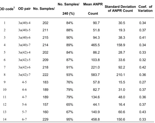
For each day, ANPR count matrices were constructed using a 1-hour time segment for each of the 14 pairs of ODs possible from Junction 3a to Junction 7 (noting that effectively, two Junction 3a origins exist). The maximum possible number of samples for each OD pair is 240 i.e. 10 days x 24 hours. For some days data were incomplete and as a result some OD pairs have less than the maximum 240 samples available. In Table I, summary statistics for the ANPR counts for the northbound traffic on the M42 study site are reported. Values are probably underestimated but what we are interested to is the value ratio between OD pairs. From this it is possible to see that the mean count (calculated over each hourly period and each day) shows considerable variability between junction pairs, with the highest values corresponding to a destination of Junction 7. This represents traffic with a more northerly destination and which is likely to involve longer journeys. The standard deviation of the ANPR count is similarly variable and appears to be associated with the size of the mean i.e. the higher the mean count the higher the standard deviation. This is illustrated through the values of the coefficient of variation, which are generally consistent at around 0.3 to 0.4. Exceptions to this are OD pairs 3, 7 and 13, which involve journeys from the two JN3a origins to JN7 (i.e. the whole route) and JN 5-7, involving traffic from the NEC exhibition junction heading Northbound.
Table I: Summary Statistics for the OD data
OD code1 OD pair No. Samples/
No. Samples/
240 (%)
Mean ANPR
Count
Standard Deviation of ANPR Count
Coef. of Variation
1 3a(40)-4 202 84% 90.7 30.5 0.34
2 3a(40)-5 211 88% 51.8 19.3 0.37
3 3a(40)-6 215 90% 94.3 38.3 0.41
4 3a(40)-7 214 89% 465.5 158.9 0.34
5 3a(42)-4 202 84% 86.2 28.7 0.33
6 3a(42)-5 209 87% 103.8 33.6 0.32
7 3a(42)-6 218 91% 221.0 92.2 0.42
8 3a(42)-7 222 93% 583.7 210.1 0.36
9 4-5 183 76% 57.8 15.5 0.27
10 4-6 189 79% 82.7 31.0 0.37
11 4-7 189 79% 134.6 48.0 0.36
12 5-6 157 65% 44.1 16.4 0.37
13 5-7 160 67% 140.9 60.6 0.43
14 6-7 229 95% 458.8 150.6 0.33
1 used as an OD pair identifier in subsequent analysis.
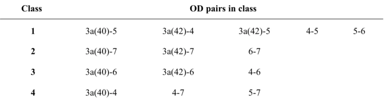
Plotting the ANPR count for each OD pair on an hourly basis throughout the day highlighted some similarities between particular pairs. As a result it was possible to form classes for similar OD pairs based on a subjective visual assessment of the plots, as reported in Table II below. In Fig. 2, plots of data for four representative OD pairs (one for each class) are shown to illustrate the typical patterns identified. Together with the mean count, the limits obtained by adding and subtracting one standard deviation to the mean are also indicated.
Class OD pairs in class
1 3a(40)-5 3a(42)-4 3a(42)-5 4-5 5-6
2 3a(40)-7 3a(42)-7 6-7
3 3a(40)-6 3a(42)-6 4-6
4 3a(40)-4 4-7 5-7
As expected with the general pattern of traffic demand, the mean ANPR count changes according to the hour and in general two peaks can be identified, corresponding to the morning (approximately 09:00) and evening (approximately 18:00). For some OD pairs the morning peak is higher, whilst for others the evening peak is higher, reflecting different structures to the demand at particular locations of the network throughout the day. The OD patterns for each of the four classes can be summarised as follows. The first class includes OD pairs with low demand throughout the day. The second class includes OD pairs that involve Junction 7 as a destination and have high demand with a pronounced peak in the evening. The third class contains OD pairs with Junction 6 as a destination and has high demand with a pronounced peak in the morning. Finally, the fourth class includes those OD pairs with clear morning and evening peaks to demand. Junctions 6 and 7 outflows therefore form a particular contribution to the pattern of demand on the M42 northbound, which has a sensible practical interpretation as Junction 6 provides a connection to Birmingham airport whilst Junction 7 feeds through to the M6 motorway and northerly destinations. The identification of the four profile classes had significance for the subsequent analysis in that it suggested that different models may be appropriate for particular OD pairs.
Fig. 2c: Jn 3a(42)-Jn 6 ANPR count profile(class 3) Fig. 2d: Jn 4–Jn 7 ANPR count profile(class 4)
B. The Variance – Mean correlation in ANPR count data
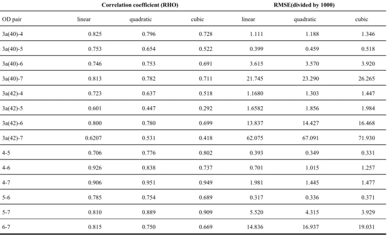
The proposed method involved the use of neural networks to produce estimates of the OD matrices. The general Neural Networks approach holds an assumption of stationary in the data (as does the classical least squares method) in order to produce good results. When the data process is non-stationary, the NN learning approach does not hold well and a transformation of the input data is required in order to obtain the best results. A study was therefore undertaken of the relationship between the mean and variance of the ANPR input data in order to investigate if a transformation would improve the NN learning process and the results obtained. It is worth noting that if a data set obtained from sources other than ANPR for training were used, it would still be desirable to investigate stationarity properties in order to obtain the best results. When the variance increases with the mean, this is an indication of non-stationarity and it may then be useful to apply variance stabilization transformations6,7. The square root, logarithmic and inverse square root transformation for example, can be applied in the case of a linear, quadratic or cubic variance - mean relationship respectively.
In Table III and Figs. 3 and 4, the correlation coefficient (indicated with RHO) and RMSE are given for each of the three transformations by OD pair. In each case a linear, quadratic or cubic model was produced of the relationship between the mean, , and variance, 2, ( ≈2, =1,2,3 respectively) and then the RHO or RMSE value calculated for the observed and predicted values from the model. The RMSE is given by
(2)
Table III: RHO and RMSE for OD variance-mean relationship
Correlation coefficient (RHO) RMSE(divided by 1000)
OD pair linear quadratic cubic linear quadratic cubic
3a(40)-4 0.825 0.796 0.728 1.111 1.188 1.346
3a(40)-5 0.753 0.654 0.522 0.399 0.459 0.518
3a(40)-6 0.746 0.753 0.691 3.615 3.570 3.920
3a(40)-7 0.813 0.782 0.711 21.745 23.290 26.265
3a(42)-4 0.723 0.637 0.518 1.1680 1.303 1.447
3a(42)-5 0.601 0.447 0.292 1.6582 1.856 1.984
3a(42)-6 0.800 0.780 0.699 13.837 14.427 16.468
3a(42)-7 0.6207 0.531 0.418 62.075 67.091 71.930
4-5 0.706 0.776 0.802 0.393 0.349 0.331
4-6 0.926 0.838 0.737 0.701 1.015 1.257
4-7 0.906 0.951 0.949 1.981 1.445 1.477
5-6 0.785 0.754 0.689 0.317 0.336 0.371
5-7 0.810 0.889 0.909 5.520 4.315 3.929
6-7 0.815 0.750 0.669 14.836 16.937 19.031
0 0.1 0.2 0.3 0.4 0.5 0.6 0.7 0.8 0.9 1
3
a
(4
2
)-5
3
a
(4
2
)-7
4
-5
3
a
(4
2
)-4
3
a
(4
0
)-6
3
a
(4
0
)-5
5
-6
3
a
(4
2
)-6
5
-7
3
a
(4
0
)-7
6
-7
3
a
(4
0
)-4
4
-7
4
-6
R
H
O linear
quadratic cubic
0 10 20 30 40 50 60 70 80
3a
(4
2)
-7
3a
(4
0)
-7
6
-7
3a
(4
2)
-6
5
-7
3a
(4
0)
-6
3a
(4
2)
-5
4
-7
3a
(4
2)
-4
3a
(4
0)
-4
4
-6
3a
(4
0)
-5
4
-5
5
-6
OD pair
R
M
S
E
linear quadratic cubic
Fig.4: Root Mean Squared Error (RMSE)/1000 for OD variance-mean relationship
III. OD ESTIMATIONUSING MIDAS DATA
The general structure of the NN model used with the M42 data has one input layer (with a linear transfer function), one hidden layer (with a hyperbolic tangent sigmoid transfer function which has the form of
and it is mapped in the interval (-1, +1) and one output layer (with a linear transfer
function). This structure is the result of many trials aimed at performing the best performance.
The type of NN model applied was a classical multi-layer feed forward neural network with the Beale-Powell conjugate gradient back-propagation training algorithm in order to improve training performance with respect to the simple back-propagation8. The algorithm adjusts the weights in the steepest descent direction where the performance function decreases most rapidly. Although the function decreases most rapidly, this does not necessarily mean the fastest convergence to a solution. In the conjugate gradient algorithm, a search is performed along conjugate directions, which generally produces a faster convergence. The input vector consisted of the flow detected on links (MIDAS data) and the output vector was given by the OD pairs constructed from ANPR counts. The dataset was divided into three subsets (two fourth for the training and one fourth for the test and one fourth for the validation set). The test set is used to stop learning and the validation one to calculate the model error.
total amount of information available for use will be compromised. In general a great care on continuity of flow data was devoted when extracting the dataset.
Considering the possibilities for using different combinations of the data available, different sampling strategies were devised based on selection of particular lanes and links from the whole set (see Table IV). The strategies were proposed in order to explore where the greatest information content in the data is and to provide a reflection of real conditions when potentially not all detectors are in working order. Obviously more strategies with a less regular step can be tested in order to better simulate real conditions but probably without adding further information. It must be stressed that flow on a link or even on a single lane of a link is functionally related to OD values and this provides the rationale behind the sampling strategy proposed by Table IV.
Table IV: Strategies for link data sampling
Strategy code
Sampling Strategy
Description
1 all links All links
2 1:8 Every eighth link
3 1:15 Every fifteenth link
4 1:30 Every thirtieth link
5 Lane 3 Fast lane for all links
6 Lane 2 Middle lane for all links
7 Lane 1 Slow lane for all links
8 ramp All ramps
In the case of “all links” strategy, the input vector has a dimension of 103 and this requires an adequate number of training samples in order to achieve a better degree of statistical significance in the fit. Because some of the other strategies also had a high input vector dimension (relative to the number of samples), it was decided to apply PCA (Principal Component Analysis) when more than 10 inputs (or links) were used for the model.
IV. MODELLINGRESULTS
In addition to the RHO and RMSE statistics the GEH value is calculated as a means of comparing results, following the approach of Taylor et al10. The GEH value allows a relative independence of scale using the following formula:
(3)
where x and y are the predicted and observed data respectively. Generally, a GEH value of 5 or less is considered acceptable and a target for model validation is that 85% of cases should have GEH < 5.
performance achieved by the use of the transformation to achieve stationarity. On the horizontal axis the OD pair code (from 1 to 14) and the sampling strategy code (from 1 to 8) are given in the format (OD code-strategy code) (see Table II for OD pair code).
The RMSE results from modelling individual OD pairs as the target output are given in Fig. 5, indicating differences obtained by using either a SQRT or Log transformation with the training data against RMSE values when the original data was used. This is clarified in Fig. 6 as calculated differences in RMSE. With the exception of some OD pairs originating at JN 3a(40), JN 3a(42) and JN 4, a transformation generally resulted in performance benefits. It is apparent that the SQRT transformation produces better results for almost all OD pairs and sampling strategies than the Log transformation. This was particularly the case for OD pair 8 (JN 3a (42) to JN 7) where a Log transform substantially worsened the performance. Similar findings were produced for the RHO statistic and so are not reproduced in detail here, however it is worthy of note that the RHO values were consistently greater than 0.7 and the average RO was calculated as 0.86, indicating strong all round performance.
The RMSE difference (Fig. 6) doesn’t consider the absolute value of the data and for this reason an evaluation in percentage terms was carried out. The ratio
(4)
was calculated, which can be considered to be a percentage RMSE (RMSE%). For the individual OD model, the RMSE% was found to be never higher than 7%; the average value being 1.4%. The highest value of this statistic was found to be produced for OD pair 8 (JN 3a(42) to JN 7) whilst for other ODs, the RMSE% values are seen to increase in line with increased standard deviation values in Table I.
0.00 100.00 200.00 300.00 400.00 1
-1 1-3 1-5 1-7 -12 2-3 2-5 2-7 3-1 3-3 3-5 3-7 4-1 -34 4-5 4-7 5-1 5-3 5-5 5-7 6-1 6-3 -56 6-7 7-1 7-3 7-5 7-7 8-1 8-3 8-5 -78 9-1 9-3 9-5 9-7
1 0 -1 1 0 -3 1 0 -5 1 0 -7 1 1 -1 1 1 -3 1 1 -5 1 1 -7 1 2 -1 1 2 -3 1 2 -5 1 2 -7 1 3 -1 1 3 -3 1 3 -5 1 3 -7 1 4 -1 1 4 -3 1 4 -5 1 4 -7
OD pair and strategy
R M S E Original SQRT Log
-200.00 -150.00 -100.00 -50.00 0.00 50.00 1
-1 1-3 1-5 1-7 -12 2-3 2-5 2-7 3-1 3-3 3-5 3-7 4-1 -34 4-5 4-7 5-1 5-3 5-5 5-7 6-1 6-3 -56 6-7 7-1 7-3 7-5 7-7 8-1 8-3 8-5 -78 9-1 9-3 9-5 9-7
1 0 -1 1 0 -3 1 0 -5 1 0 -7 1 1 -1 1 1 -3 1 1 -5 1 1 -7 1 2 -1 1 2 -3 1 2 -5 1 2 -7 1 3 -1 1 3 -3 1 3 -5 1 3 -7 1 4 -1 1 4 -3 1 4 -5 1 4 -7
OD pair and strategy
R M S E o ri g in al d a ta R M S E t ra n sf o rm ed Log SQRT
Fig. 6: RMSE differences by transformation approach (OD pair [1,4]; strategy [1,8])
It can also be seen from Figs. 5 and 6 that:
Applying a transformation to address non-stationarity can substantially improve performance for some OD pairs and offers modest improvements in the case of others. This is particularly true for OD pairs 4 (3a(40)-7) and 14 (6-7), both of which are of class 2 and characterised by high mean and standard deviation in ANPR counts;
The best sampling strategy from those considered is to use the subset of lane 1 data as an input (strategy 7), with the second best strategies being to use either lane 3 (strategy 5) or lane 2 (strategy 6). This supports the use of a lane by lane analysis and may be as a result of lane 1 having consistent levels of demand regardless of traffic conditions;
The ‘All links’ strategy generally produces the worst results compared with other strategies. This requires all detectors across all the lanes, whereby the data may be too heterogeneous to distinguish the target outputs.
Analysis based on the GEH statistic is reported in Fig. 7 and from this it can be seen that the results are variable according to the OD pair, as was the case for the RMSE statistic. OD pairs 4 (3a(40)-7), 8 (3a(42)-7) and 14 (6-(3a(42)-7) (that have the highest standard deviation in the original data) have the worst GEH values. The other OD pairs indicate a good performance with the percentage of GEH 5 always greater than 60% (and in many cases greater than 85%).
0.00 10.00 20.00 30.00 40.00 50.00 60.00 70.00 80.00 90.00 100.00 1-1 1-3 1-5 1-7 2-1 2-3 2-5 2-7 3-1 3-3 3-5 3-7 4-1 4-3 4-5 4-7 5-1 5-3 5-5 5-7 6-1 6-3 6-5 6-7 7-1 7-3 7-5 7-7 8-1 8-3 8-5 8-7 9-1 9-3 9-5 9-7 10 -1 10 -3 10 -5 10 -7 11 -1 11 -3 11 -5 11 -7 12 -1 12 -3 12 -5 12 -7 13 -1 13 -3 13 -5 13 -7 14 -1 14 -3 14 -5 14 -7
OD pair and strategy
% G E H < 5 SQRT LOG original
Fig. 7: GEH statistics for individual OD model (%GEH values less than 5) (OD pair [1,4]; strategy [1,8])
V. CONCLUSIONS
A broad summary of the findings from this study is given below.
A number of sampling strategies have been applied. In general it was found that where the model was intended to estimate individual ODs, a worse performance was found using all the data than using a more selective strategy, effectively based on one of the three lanes
The data used consisted of 14 ODs and it was possible through elementary data analysis to identify particular features of traffic demand, which resulted in 4 main OD types. The exact same patterns may not necessarily be observed if the method is applied with other data, but were an indication of the underlying variability in traffic flow levels. They also indicated that a model intended to simultaneously estimate all ODs may be less successful than one which attempted to estimate individual ODs;
An investigation of the underlying stationarity properties of the training data (an assumption of the NN modelling process) revealed non-stationarity in most of the data. Two transformations were explored in detail, the Square Root transformation and Log transformation, with comparisons being drawn against the results obtained using the original, untransformed data. In general the results obtained using the Square Root transformation outperformed those using either the original data or Log, although there were some notable exceptions to this;
ACKNOWLEDGEMENTS
The authors would like to thank the UK Highways Agency and Mott MacDonald for supplying the MIDAS and ANPR data. The views expressed in this document are those of the authors alone and are not necessary those of the Highways Agency and Mott MacDonald.
REFERENCES
1 Cascetta E (2001) Transportation Systems Engineering: Theory and Methods. Kluwer Academic Publisher, Dordrecht.
2 Camus R, Cantarella G E, Inaudi D (1997) Real-time estimation and prediction of origin—destination matrices per time slice. International Journal of Forecasting 13, Issue 1:13-19.
3 Van der Zijpp N J, De Romph E D (1997) A dynamic traffic forecasting application on the Amsterdam beltway. International journal of forecasting 13:87-103.
4 Kikuchi S, Tanaka M (2000) Estimating an origin-destination table under repeated counts of in-out volumes at highway ramps: use of artificial neural networks. TRR 1739:59-66.
5 Mussone L, Grant-Muller S and Chen H (2009) Motorway OD matrix estimation using Neural Networks, loop counts and number plate data, ITS Working paper 671, Institute for Transport Studies, University of Leeds.
6 Montgomery D C, Peck E A (1982) Introduction to Linear Regression Analysis. John Wiley & Sons, New York, NY.
7 Potts W J E (1999) Neural Network Modeling Course Notes. SAS Institute Inc., Cary, NC.
8 Beale E M L (1972) A derivation of conjugate gradients. In Lootsma F A (ed). Numerical methods for nonlinear optimization, Academic Press, London.
9 Ferrari P (1994) The instability of motorway traffic. Transp. Res. B 2 28B:175-186.


![Fig. 5: RMSE by transformation approach (OD pair [1,4]; strategy [1,8])](https://thumb-us.123doks.com/thumbv2/123dok_us/8003800.209657/10.918.171.778.632.893/fig-rmse-transformation-approach-od-pair-strategy.webp)
![Fig. 6: RMSE differences by transformation approach (OD pair [1,4]; strategy [1,8]) It can also be seen from Figs](https://thumb-us.123doks.com/thumbv2/123dok_us/8003800.209657/11.918.160.777.89.385/fig-rmse-differences-transformation-approach-pair-strategy-figs.webp)
![Fig. 7: GEH statistics for individual OD model (%GEH values less than 5) (OD pair [1,4]; strategy [1,8])](https://thumb-us.123doks.com/thumbv2/123dok_us/8003800.209657/12.918.164.756.81.425/fig-geh-statistics-individual-model-geh-values-strategy.webp)
