18th International Conference on Structural Mechanics in Reactor Technology (SMiRT 18) Beijing, China, August 7-12, 2005 SMiRT18-G02-3
3-D THERMAL WEIGHT FUNCTION METHOD AND MULTIPLE
VIRTUAL CRACK EXTENSION TECHNIQUE FOR THERMAL SHOCK
PROBLEMS
Yanlin Lu*, Xiao Zhou
*College of Mechanical & Electrical Engineering, Zhejiang University of Technology,
Hangzhou, Zhejiang 310014, P. R. China
Phone: 0571-88320091, Fax: 0571-88320130
e-mail: [email protected]
Jiadi Qu, Yikang Dou, Yinbiao He
Dept. of Component research and Design, Shanghai Nuclear Engineering Research
and Design Institute, 29 HongCao Road, Shanghai 200233, P. R. China
Phone: 021-64850220-3929, Fax: 021-64851074
e-mail: [email protected]
ABSTRACT
An efficient scheme, 3-D thermal weight function (TWF) method, and a novel numerical technique, multiple virtual crack extension (MVCE) technique, were developed for determination of histories of transient stress intensity factor (SIF) distributions along 3-D crack fronts of a body subjected to thermal shock. The TWF is a universal function, which is dependent only on the crack configuration and body geometry. TWF is independent of time during thermal shock, so the whole history of transient SIF distributions along crack fronts can be directly calculated through integration of the products of TWF and transient temperatures and temperature gradients. The repeated determinations of the distributions of stresses (or displacements) fields for individual time instants are thus avoided in the TWF method. An expression of the basic equation for the 3-D universal weight function method for Mode I in an isotropic elastic body is derived. This equation can also be derived from Bueckner-Rice’s 3-D WF formulations in the framework of transformation strain. It can be understood from this equation that the so-called thermal WF is in fact coincident with the mechanical WF except for some constants of elasticity. The details and formulations of the MVCE technique are given for elliptical cracks. The MVCE technique possesses several advantages. The specially selected linearly independent VCE modes can directly be used as shape functions for the interpolation of unknown SIFs. As a result, the coefficient matrix of the final system of equations in the MVCE method is a triple-diagonal matrix and the values of the coefficients on the main diagonal are large. The system of equations has good numerical properties. The number of linearly independent VCE modes that can be introduced in a problem is unlimited. Complex situations in which the SIFs vary dramatically along crack fronts can be numerically well simulated by the MVCE technique. An integrated system of programs for solving the thermal shock problems by means of the TWF method was developed. By means of such a system, a series of histories of transient SIF distributions along 3-D crack fronts with different crack depth and crack aspect ratios subjected to different thermal shock conditions were solved. Examples show that the scheme is of high efficiency and of good accuracy.
function, universal weight function method.
1. INTRODUCTION
3-D cracks occur frequently in reactor vessels and piping. The assessment of safety of such structures subjected to pressurized thermal shock is an important problem. In order to evaluate the safety of such structures correctly, it is demanded to determine the variations of distributions of transient stress intensity factors (SIFs) along the whole crack front for various thermal shock conditions. The major difficulty in calculating the variation of transient SIF distributions is that a large amount of computation works will usually be involved. To solve such a problem, two methods have been developed. One is the direct method through analysis of thermo-elasticity. By this method, after the transient temperature fields have been determined for specific times, the SIF distributions for these times are determined from the results of stress or displacement fields for the cracked body through repeated analyses of thermo-elasticity. These analyses would be performed by analytical or numerical procedures, e.g. by finite element method (FEM) or by boundary element method (BEM). Since the existence of cracks and the rapid variation and high gradient of temperature fields, the computation procedure is usually tedious, time consuming and expensive. Another is the well-known weight function (WF) method based on the principle of superposition.
The WF concept was introduced by Bueckner (1970), and serves as a Green’s function for the linear elastic crack tip opening mode (Mode I) SIF KI for an arbitrary distribution of crack face traction. Subsequently, many
contributors, e.g. Rice (1972,1985a,1985b), Bueckner (1973, 1987), Wu and Carlsson (1983), Bortman and Banks-Sills (1983), Sham (1987), Sham and Zhou (1989), Glinka and Shen (1991), Fett and Munz (2000), and Wang and Lambert (2001), extended the theory to more generalized forms. The contributions have covered the 2-D, 3-D, mixed mode, graded material and displacement boundary condition problems. This leads to the representation
∫
∫
∫
⋅ Σ− ⋅ Σ+ ⋅=
Σ
Σ V V
K
u t
d d
d α α
α
α t h u t f h (1)
Here V is the volume of the body, Σt is the bounding surface of V with prescribed traction t, Σu is the bounding
surface of V with prescribed displacements u and f is the body force. The WF hα can be determined from known
reference displacement fields and reference SIFs for some reference loading. In Eq. (1), tα is the traction
generated by the weight function hα on Σu, and subscripts α = 1, 2, and 3, denotes Mode I, Mode II, and Mode
III, respectively. We shall refer to these types of weight functions as mechanical weight functions (MWFs) for distinguishing from the following mentioned thermal weight function (TWF).
The MWF method is a powerful and efficient method for determining the SIFs for a cracked body subjected to mechanical loading. The WF is a universal function for a specified crack tip and body geometry. Once the WF for the specific crack tip and body geometry is known, the SIF for that crack body subjected to any mechanical loading can be simply calculated by direct integration through Eq. (1). If the MWFs were known, and the loads were mechanical only and did not vary with time, these computations could usually be done by the MWF method with little efforts. However, when transient problems, such as problems of cracked bodies subjected to thermal shock, are to be solved, in order to understand the whole variation of transient SIFs, repeated determinations of the distributions of stress fields for a prospected uncracked body have to be performed. The difference of the MWF method from the direct method is lying only on the fact that, for the MWF method, the stress analyses need to be performed simply for the corresponding uncracked body, and only the distributions of stresses along the prospective crack face need to be determined. The computation is still tedious and time-consuming when the body geometry or load condition is complex and numerical procedures such as FEM or BEM are used.
The TWF scheme was proposed in Eq. (28) of Rice’s paper (1985a) by a framework of transformation strain, in which the “weight” is the divergence of hα. The TWF scheme has some advantages for solving thermal
stress, plane strain and axisymmetric problems.
The determination of WFs for a 3-D crack problem is generally rather formidable. The difficulty is that the SIFs along a 3-D crack front are usually unknown functions of positions and the WF hα in Eq. (1) will not be
determined as explicit functions except for some simple configurations. A variety of numerical procedures have been developed for determination of WFs. Taking for examples, the procedure developed by Bueckner (1973) was based on expressing the WF in terms of integral equations. The procedure developed by Paris and McMeeking (1975) was based on standard FEM by removing a cylinder of material centered at the crack tip. The procedure developed by Sham (1987) was based on the FEM by using the variational principle for determining the singular fields in finite bodies. The procedure developed by Vanderglas (1978) and Parks and Kamenetzky (1979) was based on the virtual crack extension (VCE) technique. The procedure developed by Zhao and Wu (1989a,b) and Zhao and Newman et al. (1998) was based on the slice synthesis technique. The procedure developed by Vainshtok and Varfolomeyev (1990) was based on the VCE concept and a technique of expressing the geometric correction factor as the sum of some linearly independent functions. In Vainshtok and Varfolomeyev’s (1990) work, elliptical crack geometries were studied. Five kinds of “crack front translations”, two for elliptical expansions along it’s principal axes and two for rigid translations along these axes and one for rigid rotation about it’s center, were used to define the VCEs. Then, five kinds of linearly independent functions,
of the form , were used to represent the variation of unknown SIFs along crack fronts.
Because of the global nature of these VCEs as well as of these interpolation functions, the method could only work well for load cases when the actual variations of unknown SIFs could be approximately represented by these particular functions. If the unknown SIFs vary dramatically along crack front, which will always occur during thermal shock, the method would result in large errors.
) 2 , 1 , 0 , ( cos
sinmt⋅ nt mn=
In the present paper, an expression of the basic equation for the 3-D universal WF method for Mode I in an isotropic elastic body is derived, which can directly be used for numerically determining the distributions of SIFs along 3-D crack fronts for both mechanical and thermal loading. Then, a novel technique, which will be referred to as Multiple Virtual Crack Extension (MVCE) technique, is proposed to solve the basic equation of TWF. An unlimited number of linearly independent VCEs, which have local nature, can be introduced in the present method. In addition, a special discrete approximation for unknown SIFs is introduced to solve the basic equations in 3-D TWF method, which is similar to the technique used in FEM but the “shape functions” used are directly concerned with the corresponding VCE modes. As a result, a triple-diagonal coefficient matrix is obtained for the basic system of equations of 3-D TWF method. It has good numerical properties. The situations, in which unknown SIFs vary dramatically along crack fronts, such as in the case of thermal shock, can be numerically well simulated.
It can also be understood from the basic equation that the thermally induced SIF is not only dependent on the temperature on the bounding surface, but also is dependent on the temperature gradient in the volume. The integration in the TWF scheme will be carried out around the boundary as well as over the volume. Same as in the previous work (Lu, 2001) in plane stress, plane strain and axisymmetic cases, the scheme in 3-D cases is also based on an integrated program system of finite element implementations. Examples show that high efficiency and good accuracy can be achieved.
2. BASIC EQUATION OF UNIVERSAL WF METHOD FOR MODE I CRACK PROBLEMS
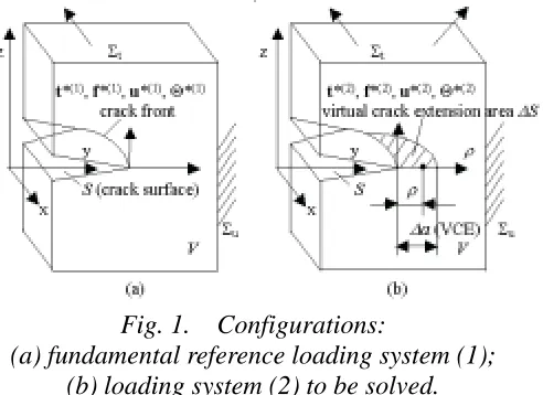
The WF for Mode I can be calculated from a known solution of a fundamental reference loading system. Fig. 1a shows an isotropic elastic body which is subjected to a known fundamental reference (Mode I) loading system (1), containing a prescribed traction t*(1) at boundary Σt, a prescribed displacement u*(1)
at boundary Σu, a body force f*(1) and a thermal
loadΘ*(1). Here, the thermal load Θ *= T0-T, T0
being a certain reference temperature, T being the actual temperature. The variation of the SIF
KI(1) along the crack front is known. Fig. 1b
shows the same cracked body which is subjected to another (Mode I) loading system (2), containing a prescribed traction t*(2) at boundary Σt, a prescribed displacement u*(2) at boundary Σu, a body force f*(2) and a thermalload
Fig. 1. Configurations:
Θ *(2)
. The variation of the SIF KI(2) along the crack front is to be solved. According to Betti’s reciprocal theorem,
we have derived an expression for a 3-D weight function (including TWF) method for Mode I crack problems (Lu, 2001),
∫
∫
∫
∫
∫
+ Θ ⋅∂∂ ∂ ∂ ⋅ + Σ ∂ ∂ ⋅ − Σ ∂ ∂ ⋅ = − ∆∆ ∆ Σ Σ V
kk V S I I dV S dV S d S d S d a H K K
S t u
) 1 ( ) 2 ( * ) 1 ( ) 2 ( * ) 1 ( ) 2 ( * ) 1 ( ) 2 ( * ) 2 ( ) 1 ( 4
1 σ α σ
ρ ρ π u f t u u t (2)
Here H is the appropriate elastic modulus,
− ), for planestrain 1 ( stress plane for , 2 ν E E
H (3)
E is Young’s modulus, ν is Poisson’s ratio, and α is the thermal expansion coefficient. S is the area of the crack face, V is the volume of the body surrounded by the bounding surface Σ, Σ=Σt∪Σu, and ∆S is a VCE.
The VCE can be described by an infinitesimal crack front advance variation δa(s) along the whole crack front Γ, (cf. Fig.2),
l s g s a δ δ ( )= ( ) ( Here 4)
s is the arc length along the crack front, a(s) is the local crack length measured normal to the crack front, g(s) is a normalized extension function for describing the distribution of the crack front advance, and l is a selected characteristic crack length measure, δl is the characteristic measure of the variation δa(s). The integral of the left-hand side of Eq. (2) is along the crack face (one side only). dσ is the differential area on ∆S. σkk is the first invariant of the reference stress tensor. ρ is the normal
distance of th onsidered point (within ∆S during integration) from the crack front, and ∆a is the local VCE of the crack length normal to the crack front at the corresponding crack tip, that is, a a(s)
e c
δ
=
∆ . Note the fact that
ds d dσ = ρ
) ( 2 ) (
0 d a s
a s a δ π ρ ρ ρ δ = − ∆
∫
(5) For a particular VCE, ∆S, we can express the partial derivatives that∂[L]=∂[L]⋅ δl
S l
S ∂ ∆
∂ (6)
Substituting these into Eq. (2), the equation becomes
∫
∫
∫
∫
∫
+ Θ ⋅∂ ∂ ∂ ∂ ⋅ + Σ ∂ ⋅ − Σ ∂ ⋅ = Σ Σ Γ V kk V I I dV l dV l d l d l ds s a Hl t u
) 1 ( ) 2 ( * ) 1 ( ) 2 ( * ) (
1 δ α σ
δ u f u t (2) ∂ ∂ K
K *(2) (1)
) 1 ( ) 2 ( * ) 2 ( ) 1 (
2 u t
(7)
Eq. (7) is not generally used directly in practice to calculate KI , because σkk is sensitive to crack front
e
variation and the partial derivative in the equation is unlikely to be determin d. For 3-D isotropic elastic problems, ) 1 ( ∂ ∂ + ∂ ∂ + ∂ ∂ − = − = z w y v x u E E kk kk ) 1 ( ) 1 ( ) 1 ( ) 1 ( 2 1 2
1 νε ν
σ (8)
Here u, v and w are displacements in the directions of global coordinates x, y and z. Substituting Eq. (8) into Eq. (7), changing the order of differentiation and noting that
∂ ∂u ∂ ∂v ∂ ∂w
) 2 ( * ∂ ∂ ∂ Θ ∂ + ∂ ∂ ∂ Θ ∂ + ∂ ∂ ∂ Θ ∂ − ∂ ∂ Θ ∂ ∂ + ∂ ∂ Θ ∂ ∂ + ∂ ∂ Θ ∂ ∂ = ∂ ∂ +∂ ∂ +∂ ∂ Θ l w z l v y l u x l w z l v y l u x l z l y l x ) ( ) ( )
( *(2) *(2) *(2) ) 2 ( * ) 2 ( * ) 2 ( * α α α α α α α (9)
using Gauss’s theorem, the following equation can be deduced.
(10)
Fig. 2. Virtual crack
extension
∂ ∂ ⋅ Θ ∇ − Σ ⋅ ∂ ∂ Θ + ∂ ∂ ⋅ + Σ ∂ ⋅ − Σ ∂ ⋅ =∫
∫
∫
∫
∫
∫
Σ Σ Σ Γ dV l d l E dV l d l d l ds s a H l V V u t ) 1 ( ) 2 ( * ) 1 ( ) 2 ( * ) 1 ( ) 2 ( * ) ( 2 1 ) ( u n u u f u t α α ν δ δ ∂ ∂ KKI I (1)
) 2 ( * ) 1 ( ) 2 ( * ) 2 ( ) 1 ( 2
) 1 (
Here, is the normal of the bounding surface. The fourth integral on the right-hand side of Eq. (10) is composed of 2 parts, namely, the integrals on Σ
n
l
∂
t and on Σu. The latter vanishes because the components of
in the directions of the prescribed displacements are always zeros. (Other directions having no prescribed displacement should be treated as Σ
∂u /
t). So, Eq. (10) can also be written as
∂ ∂ ⋅ Θ ∇ − Σ ⋅ ∂ ∂ Θ + ∂ ∂ ⋅ + Σ ∂ ∂ ⋅ − Σ ∂ ∂ ⋅ =
∫
∫
∫
∫
∫
∫
Σ Σ Σ Γ dV l d l E dV l d l d l ds s a H K K l V V I I t u t ) 1 ( ) 2 ( * ) 1 ( ) 2 ( * ) 1 ( ) 2 ( * ) 1 ( ) 2 ( * ) 1 ( ) 2 ( * ) 2 ( ) 1 ( ) ( 2 1 ) ( 2 1 u n u u f t u u t α α ν δ δ (10’)Eq. (10) or Eq. (10’) is the basic equation of the universal WF method for Mode I crack problems in an isotropic elastic body. This equation can directly be used for determination of the distribution of the SIF KI(2)
along a 3-D crack front (cf. the next section). It can be understood from Eq. (10) that the so-called TWF is in fact coincident with the MWF except for some constants of elasticity. They are all with a form . In the TWF scheme, the “thermal loading” means the thermal strain and the gradient of thermal strain (or the temperature and the temperature gradient). It can also be understood that the thermally induced SIF is not only dependent on the temperature on the bounding surface, but also dependent on the temperature gradient in the volume. The integration should be carried out around the whole boundary and over the whole volume.
l
∂ ∂u(1)/
It should be mentioned that Eq. (10) or Eq. (10’) could also be derived from Bueckner-Rice’s 3-D WF formulations in the framework of transformation strain. The Eq. (A7) in Rice’s paper (1972) could be rewritten as (in the present notations)
∫
∫
∫
= ⋅ Σ+ ⋅Σ
Γ a V a
I I dV d ds s a H K
K (2) (1) (2) (1) ) 2 ( ) 1 ( ) ( 2 u f u
t δ δ
δ (11)
Here the notationδa(L)denotes the first order variation in the quantity , viewed as a function of crack position and some other variables, when only the crack position is varied. Considering the situation having the boundary condition of prescribed displacements, and following an analogous procedure for deriving Eq. (8.5) in Bueckner’s paper (1987), Eq. (11) should become
) (L
∫
∫
∫
∫
= ⋅ Σ− ⋅ Σ+ ⋅ Σ ΣΓ a a V a
I
I a sds d d dV
H K K u t ) 1 ( ) 2 ( * ) 1 ( ) 2 ( * ) 1 ( ) 2 ( * ) 2 ( ) 1 ( ) ( 2 u f t u u
t δ δ δ
δ (12)
Again, following the same procedure in Eqs. (18)-(22) in Rice’s paper (1985a), for an isotropic elastic body, an effective body force
− Θ −∇ = ν α 2 1 ) 2 *( eff E
f (13)
should be introduced in the volume V. Furthermore, an effective traction
n t ν α 2 1 ) 2 *( eff − Θ
= E (14)
should be introduced on the bounding surface Σ. Now, for a particular crack front advance expressed by Eq. (4),
l l a δ δ ∂ ∂ = ( ) )
(L L (15)
and substituing Eqs. (13)-(15) into Eq. (12), one obtains Eq. (10).
3. NUMERICAL PROCEDURES FOR DETERMINATION OF DISTRIBUTIONS OF SIFS ALONG A 3-D CRACK FRONT
The distribution of the SIF KI(2) along the crack front is solved through finite element (FE) implementation
in this paper. Though the following proposed numerical procedure would be applicable for both mechanical and thermal loading, for simplicity, only the thermal loading is to be considered and appears in the following equations. In this case, Eq. (10) becomes
∂ ∂ ⋅ Θ ∇ − Σ ⋅ ∂ ∂ Θ =
∫
∫
∫
Γ Σ l d l dVE ds s a H K K l V I I ) 1 ( ) 2 ( * ) 1 ( ) 2 ( * ) 2 ( ) 1 ( ) ( 2 1 ) ( 2 1 u n u α α ν δ
δ (16)
3.1 Multiple virtual crack extension (MVCE) technique
For 3-D crack problems, KI(1)and KI(2) vary along the crack front. They cannot be simply separated from
can
novel technique, which will be referred to as the multiple virtual crack extension (MVCE) technique, is proposed here.
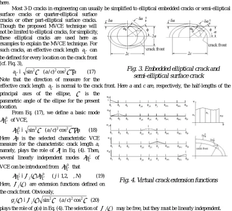
Most 3-D cracks in engineering can usually be simplified to elliptical embedded cracks or semi-elliptical surface cracks or quarter-elliptical surface
cracks or other part-elliptical surface cracks. Though the proposed MVCE technique will not be limited to elliptical cracks, for simplicity, these elliptical cracks are used here as examples to explain the MVCE technique. For such cracks, an effective crack length aφ
be defined for every location on the crack front (cf. Fiq. 3),
a c
a
aφ = sin2φ+( / )2cos2φ⋅ (17) Note that the direction of measure for the
effective crack length is normal to the crack front. Here a and c are, respectively, the half-lengths of the principal axes of the ellipse,
φ
a
φ is the parametric angle of the ellipse for the present location.
Fig. 3. Embedded elliptical crack and
semi-elliptical surface crack
From Eq. (17), we define a basic mode of VCE, 0 φ δa a c a
a φ φ δ
δ φ0 = 2 + 2 2 ⋅
cos ) / (
sin (18)
Here δa is the selected characteristic VCE measure for the characteristic crack length a, namely, plays the role of δl in Eq. (4). Then, several linearly independent modes of
VCE can be introduced from that
j aφ δ 0 φ δa ) , , 2 , 1 ( )
( a0 j N
a j j L = = φ φ ω φ δ δ ) ( (19)
Here, ωj φ are extension functions defined on
the crack front. Obviously,
Fig. 4. Virtual crack extension functions
φ φ
φ ω
φ 2 2 2
cos ) / ( sin ) ( )
( a c
gj = j + (20)
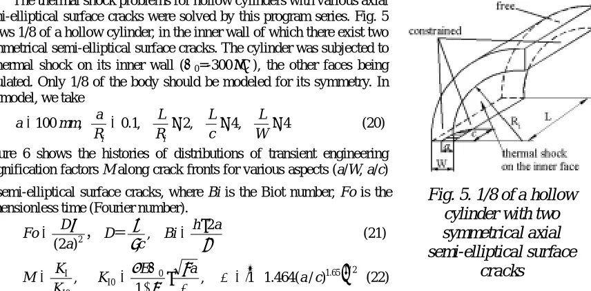
plays the role of g(s) in Eq. (4). The selection of ωj(φ) may be free, but they must be linearly independent. In this paper, the ωj(φ) will be defined as follows. Introduce arbitrarily N points on the crack front, for which the SIFs are to be determined, and for which the parametric angle of the ellipse is denoted as
) , , 2 , 1 ( j N
j = L
φ . The crack front is thus divided into N-1 sections (cf. Fig. 4). Let
< ≤ ≤ − = ) ( 0 ) ( 2 1 ) ( 2 2 1 1 1 φ φ φ φ φ ξ φ
ω , (21a)
) 1 , , 3 , 2 ( , ) ( 0 ) ( 2 1 ) ( 2 1 ) ( 0 ) ( 1 1 1 1 1 − = < ≤ ≤ − < ≤ + < = + + N j j j j j j j-j L φ φ φ φ φ ξ φ φ φ ξ φ φ φ
ω (21b)
, ) ( 2 1 ) ( 0 ) ( 1 -1 -1 ≤ ≤ + < = − N N N N
N ξ φ φ φ
φ φ φ
ω (21c)
2 1, 1 1, ( 1,2, , 1) 1 − = ≤ ≤ − − − − = + N k k k k k
k φ φ ξ L
φ φ
ξ (21d)
The extension functions ωj(φ) have a special property that they satisfy the basic needs for use as shape functions in discrete approximations,
∑
(22)= = ≠ = = = N j j ij i j j i j) (i 1 1 ) ( , ) ( 0 1 ) (φ δ ω φ ω
Thus, they can directly be used as shape functions to approximately represent the variation of any variable defined on the crack front.
According to this property, we may write
(1) (2)
I
I K
K =Ψ⋅ (23)
∑
= = Ψ N i i i A 1 ) (φω (24)
Here,Ai are some unknown coefficients. Substituting Eqs. (23), (24) into Eq. (16), and noting that
ds=c sin2φ+(a/c)2cos2φ⋅dφ (25) the left-hand side of Eq. (16) (denoted as Ileft) becomes
[ ]
ω φ δ φ φ φδ φ
φ
φ H K A a a c d
c a I N N i i i I 2 2 2 1 2 ) 1 (
left ( ) sin ( / ) cos
2 1 1 + ⋅ ⋅ =
∫
∑
= (26)Now, for a particular definition of VCE, the corresponding VCE mode has already been expressed in Eq. (18) and Eq. (19). Substituting these into Eq. (26), we have
j aφ
δ
φ ω φ
[ ]
ω φ[
φ φ]
φφ H A K a c d
c I j N i I i i
N 2 2 2
1
2 ) 1 (
left ( ) ( )sin ( / ) cos
2 1 + ⋅ =
∫
∑
= (27)Substituting these into Eq. (16), the following equations can be deduced
[ ]
[
]
j N a V j I i N i i dV a d a E d c a K H c A φ δ φ φ ω φ ω φ φ φ φ ν α α ∂ ∂ ⋅ Θ ∇ − Σ ⋅ ∂ ∂ Θ = +∫
∫
∫
∑
= Σ ) 1 ( ) 2 ( * ) 1 ( ) 2 ( * 2 2 2 2 ) 1 ( 1 ) ( 2 1 cos ) / ( sin ) ( ) ( 2 1 u n u ) , , 2 , 1(j= L N (28) Simply rewritten, this yields the form
) 2 1 1 ,N , , j ( D A C j N i i
ij = = L
∑
=
(28’)
This is a system of equations with respect to unknown coefficients . Solving from this system of equations, and substituting them into Eq. (23) and Eq. (24), the distribution of K
i
A Ai
I(2) along the whole crack front is
obtained.
The MVCE technique proposed here possesses some notable features. The first is that the interpolation of unknown variable KI(2) is directly concerned with the VCE modes, that is, the specially selected extension
functions ωj(φ) of the VCEs are directly used as the shape functions for the interpolation of KI(2). The second
is that the number of linearly independent VCE modes, which can be introduced in a problem, is unlimited. The selection of locations φj and the corresponding VCE modes ωj(φ) can be free, as long as they are linearly
independent and satisfy some basic needs for the shape functions. This means that, for a particular problem, the number of unknown coefficients and the locations at which the SIF will be calculated can be selected freely according to the details of the problem such as the accuracy required and the variation aspects of the SIF to be calculated. We could select fine divisions where the SIF varies dramatically, and select coarse divisions where the SIF varies smoothly. The third feature is that the resultant coefficient matrix of the final system of equations (Eq. (28)) is a triple-diagonal matrix and the values of the coefficients on the main diagonal are large. This means, the system of equations has good numerical properties. The error of the known reference SIF KI(1) at a
particular location will have a direct effect only on the results of KI(2) at that location and at adjacent locations. It
will have little effect on the results of KI(2) at all other distant locations. For example, for a semi-elliptical surface
crack, the singularity of the stress field at the intersection point of the crack front with the surface of the body is not r-1/2. The value of KI(1) there has only a meaning for reference. Moreover, the crack mode there is not pure
such as used by Vainshtok and Varfolomeyev (1990) in the MWF scheme, were used, the errors on the value of K
t
t n
m cos
sin ⋅
I(1) and the errors caused by the equation invalidity would cause significant effects on the results
of KI(2) at all locations on the crack front. However, in the present method, since the matrix is triple-diagonal, the
effect would be limited to a small region near that location. Because of these advantages, the complex situations in which the SIFs vary dramatically along crack fronts, such as thermal shock, can be numerically well simulated by the present technique.
, 100
=
R a mm
i
τ
a D
Fo
) 2 ( 2
=
I , K
K K
M =
3.2 Calculation of the WF and the stiffness derivative method
The stiffness derivative technique (Lu et al., 2001), which was used in the MWF scheme (Vanderglas, 1978), also named as the virtual crack extension technique (Parks and Kamenetzky, 1979), was used to calculate the WF (the rate of change ∂u(1)/ a). The procedure and formulations are straightforward 3-D extensions of those listed in Lu, et al. (2001) for 2-D cases. The details are omitted here.
∂
4. NUMERICAL EXAMPLES AND DISCUSSION
It can be found from Eq. (28), that the SIF in the TWF formulations is not only dependent on the temperature, but also on the temperature gradient. The integration in the TWF method has to be carried out around the whole boundary as well as over the whole volume. It is practical and useful to develop an integrated numerical procedure for directly calculating the TWF and the integration. A series of 3-D programs based on the finite element formulation have been developed. The series includes a finite element auto-modeling system, a transient and steady state temperature analysis program, a structural analysis program, a TWF analysis program and a thermal SIF analysis program. The last two were designed as post-processors.
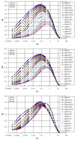
The thermal shock problems for hollow cylinders with various axial semi-elliptical surface cracks were solved by this program series. Fig. 5 shows 1/8 of a hollow cylinder, in the inner wall of which there exist two symmetrical semi-elliptical surface cracks. The cylinder was subjected to a thermal shock on its inner wall (Θ0=-300°C), the oth faces being
insulated. Only 1/8 of the body should be modeled for its symmetry. In the model, we take
er
4 , 4 , 2 , 1 .
0 ≥ ≥ ≥
=
W L c
L R
L a
i
(20)
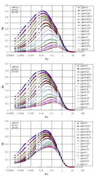
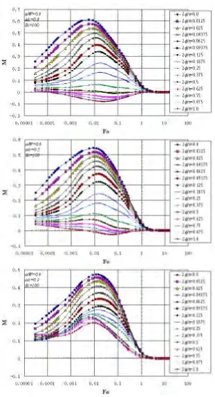
Figure 6 shows the histories of distributions of transient engineering magnification factors M along crack fronts for various aspects (a/W, a/c) of semi-elliptical surface cracks, where Bi is the Biot number, Fo is the dimensionless time (Fourier number).
λ ρ
λ h a
Bi c
D , = ⋅2 (21)
[
1.65]
1/20 0
I , 1 1.464( / )
1 a c
a E
+ = Φ Φ ⋅ −
Θ
= π
ν α
(22)
Fig. 5. 1/8 of a hollow
cylinder with two
symmetrical axial
semi-elliptical surface
cracks
0 I
Here τ is the time, λ is the thermal conductivity, ρ is the density, c is the specific heat, h is the heat transfer coefficient at the surface subjected to thermal shock. The effects of temperature on material properties were neglected in these preliminary calculations. E=210Gpa, ν=0.3, α=12.5×10-61/K, λ=42W/mK, D=11.63mm2/Sec. The uniform crack face pressure was taken as the fundamental reference loading. The reference SIFs KI(1) were
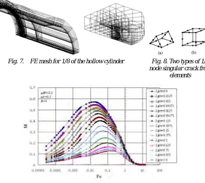
directly calculated by the COD method (Lu, 1996) from results of finite element (FE) analyses. Fig. 7 shows the FE meshes used in the FE analyses. The mesh pattern near crack fronts had been optimized by previous studies for surface cracked plate problems (Lu, 1996,1997). The 20-node isoparametric elements were used everywhere, but two types of crack front singular elements were used for different purposes of computation. The 1/4 node singular triangular prism element (Fig. 8a) is used for the first pass of computation of displacement analysis of the fundamental reference loading system in order to get the stress intensity factor KI(1) accurately. The 1/4 node
singular hexahedron element (Fig. 8b) is used for the 2nd pass of computation of displacement analysis of the fundamental reference loading system, which is then used for computing the TWF and for integration for convenience.
um differ
extract the SIF in the direct thermo-elastic analyses. The accuracy of the COD method had been previously checked (Lu, 1997). Table 1 shows the percentage differences of the results obtained by the COD method and by the MVCE method at the selected times. Because some values of M are nearly zero, the percentage of the difference listed in the table is related to the maximum values of M along the whole crack front at that time instance. The differences between the two methods at most locations and times are less than 3%. The maxim
ence is 6.34%. (Here, the values of M for φ=0 are the extrapolated values from two adjacent values). The histories of the SIF distributions will also be influenced by thermal shock conditions. Figure 9 shows the result for Bi=1 and the crack configuration of a/W=0.5 and a/c=0.5. Comparing Figure 9 with the corresponding figure for Bi=100 and a/W=0.5 and a/c=0.5, it could be seen that the maximum values have chang
al shock correctly, it is necessary to understand the histories of SIF distributions along
a ed.
It could be seen from Figures 6 and Figure 9 that the variations of distributions of transient SIFs along 3-D crack fronts are complex. Take the configuration of a/W=0.2 and a/c=0.2 for example. The location at which the maximum SIF occurs is firstly at the intersection point C of the crack front with the plate surface, but it is gradually shifted to the deepest point A. For other configurations, possibly this shift will not occur. It could also be seen from Figure 6 that the time when the maximum SIF value occurs varies with crack configuration and thermal shock condition. It is necessary to determine the actual time when the maximum SIF will occur. When engineering approximate approaches, e.g. those proposed in BS7910, are to be used, the correct determination of this time and the corresponding temperature field will be the first step. In order to evaluate the safety of a 3-D cracked body subjected to therm
the crack fronts in detail.
The most interested advantage of the TWF method is that it is of very high efficiency. For an engineering problem, several thermal shock conditions (e.g. N conditions) would usually be considered. If such a problem is solved by direct analyses through thermo-elasticity (e.g. by the COD method) or by the MWF method, a large amount of computation will usually be involved. Most of the computation times will be spent on the analyses of stress or displacement fields. However, if the TWF method were used, little work would be involved. Table 2 shows comparisons of computation time needed by the COD method and by the TWF method for solving a problem of a 3-D cracked hollow cylinder (like that in Figure 6) if N therm l shock conditions and M time instants are considered. If all SIFs were calculated by the COD method, M×N times of repeated FE stress analyses would have to be performed after the transient temperature fields had been determined. These stress analyses would have to be performed by numerical procedures such as FEM or BEM. However, if the TWF method were used, only N+3 times of computations would be needed (2 for displacement analyses for the reference loading system (1), 1 for TWF calculation, and N for integration for the N thermal shock conditions). The work could automatically be done by means of a series of programs. It is of very high efficiency to use the TWF method. In the meanwhile, good accuracy was achieved. Though the TWF method has a drawback that the integration should be carried out around the whole boundary and over the whole volume of the body, by means
f a series of integrated programs, the TWF method is still convenient for use in practical engineering.
l simulated by the MVCE technique. Examples show that e scheme is of high efficiency and of good accuracy.
o
5. CONCLUSIONS
In this paper, an expression of the basic equation for the 3-D universal WF method for Mode I in an isotropic elastic body is derived, which can directly be used for numerically determining the distribution of SIFs along 3-D crack fronts for both mechanical and thermal loading. This equation can also be derived from Bueckner-Rice’s 3-D WF formulations in the framework of transformation strain. It can be understood from this equation that the so-called TWF is in fact coincident with the MWF except for some constants of elasticity. Then, a novel technique, which will be referred to as multiple virtual crack extension (MVCE) technique, is proposed to solve the basic equations in the 3-D universal WF method. The MVCE technique possesses several advantages. The specially selected linearly independent VCE modes can directly be used as shape functions for the interpolation of unknown SIFs. As a result, the coefficient matrix of the final system of equations in the MVCE method is a triple-diagonal matrix and the values of the coefficients on the main diagonal are large. The system of equations has good numerical properties. The number of linearly independent VCE modes that can be introduced in a problem is unlimited. For a particular problem, the number of unknown coefficients and the locations at which the SIF will be calculated can be selected freely according to the details of the problem such as the accuracy required and the variation aspects of the SIF. Complex situations in which the SIFs vary dramatically along crack fronts can be numerically wel
th
ACKNOWLEDGEMENTS
lso supported by Research Center of Science at Zhejiang University of Technology under Grant No. 199910.
and Grand No. 50075083 and by Zhejiang Provincial Natural Science Foundation of China under Grant No. 595080. The work was a
k fronts f
Fig. 6(a) Histories of M along crac
or crack configuration of a/W=0.2 and
k fronts f
Fig. 6(b) Histories of M along crac
or crack configuration of a/W=0.5 and
Fig. 7. FE mesh for 1/8 of the hollow cylinder
Fig. 8. Two types of 1/4
node singular crack front
elements
Fig. 9. Histories of M for a/W=0.5 and a/c=0.5 and Bi=1
REFERRENCES
1. Bortman, Y., and Banks-Sills, L., (1983). An extended weight function method for mixed-mode elastic crack analysis. Journal of Applied Mechanics, 50, 907-909.
2. Bueckner, H. F., (1970). A novel principle for the computation of stress intensity factors. Zeitschrift fur Angewandte Mathematik und Mechanika, 50, 529-546.
3. Bueckner, H. F., (1973). Field singularities and related integral representations. In Mechanics of Fracture I: Methods of analysis and Solution of Crack Problems (Edited by Sih, G. C.), 239-314, Noordhoff, Leyden. 4. Bueckner H. F., (1987). Weight functions and fundamental fields for the penny-shaped and the half-plane
crack in three-space. International Journal of Solids and Structures, 23, 57-93.
5. Fett, T., and Munz, D., (2000). Applicability of the extended Petroski-Achenbach weight function procedure to graded materials. Engineering Fracture Mechanics, 65, 393-403.
6. Glinka, G., and Shen, G., (1991). Universal features of weight functions for cracks in mode I. Engineering Fracture Mechanics, 40, 1135-1146.
7. Lu, Y.-L., (1996). A practical procedure for evaluating SIFs along fronts of semi-elliptical surface cracks at weld toes in complex stress fields. International Journal of Fatigue, 18, 127-135.
8. Lu, Y.-L., (1997). Distributions of SIFs for symmetrical part-elliptical and semi-elliptical surface cracks in plates subjected to crack face shear loading, International Journal of Fatigue, 19, 421-427.
9. Lu, Y.-L., Liu, H., Jia, H., Yu, Z.-Q., (2001). Finite element implementation of thermal weight function method for calculating transient SIFs of a body subjected to thermal shock, International Journal of Fracture, 108, 95-117.
10. Paris, P. C., and McMeeking, R. M., (1975). Efficient finite element methods for stress intensity factors using weight functions. International Journal of Fracture, 11, 354-358.
Journal for Numerical Methods in Engineering, 14, 1693-1705.
12. Rice, J. R., (1972). Some remarks on elastic crack-tip stress fields. International Journal of Solids and Structures, 8, 751-758.
13. Rice, J. R., (1985a). Three-dimensional elastic crack tip interactions with transformation strains and dislocations. International Journal of Solids and Structures, 21, 781-791.
14. Rice, J. R., (1985b). First-order variation in elastic fields due to variation in location of a planar crack front.
Journal of Applied Mechanics, 52, 571-579.
15. Sham, T.-L., (1987). A unified finite element method for determining weight functions in two and three dimensions. International Journal of Solids and Structures, 23, 1357-1372.
16. Sham T.-L., and Zhou, Y., (1989). Weight functions in two-dimensional bodies with arbitrary anisotropy.
International Journal of Fracture, 40, 13-41.
17. Tsai, C.-H. and Ma, C.-C., (1992). Thermal weight function of cracked bodies subjected to thermal loading.
Engineering Fracture Mechanics, 41, 27-44.
18. Vanderglas, M. L., (1978). A stiffness derivative finite element technique for determination of influence functions. International Journal of Fracture, 14, R291-294.
19. Vainshtok, V. A., and Varfolomeyev, I. V., (1990). Stress intensity factor analysis for part-elliptical cracks in structures. International Journal of Fracture, 46, 1-24.
20. Wang, X., and Lambert, S. B., (2001). Semi-elliptical surface cracks in finite-thickness plates with built-in ends. II. Weight function solutions. Engineering Fracture Mechanics, 68, 1743-1754.
21. Wu, X. R., and Carlsson, J., (1983). The generalized weight functions method for crack problems with mixed boundary conditions. Journal of the Mechanics and Physics of Solids. 31, 485-497.
22. Zhao, W., Newman, J. C. Jr, Sutton, M. A., Shivakumar, K. N., and Wu, X. R., (1998). Stress intensity factors for surface cracks at a hole by a three-dimensional weight function method with stresses from the finite element method. Fatigue & Fracture of Engineering Materials & Structures, 21, 229-239.
23. Zhao, W., Wu, X. R., and Yan, M. G., (1989a). Weight function method for three dimensional crack problems---I. Basic formulation and application to an embedded elliptical crack in finite plates. Engineering Fracture Mechanics, 34, 593-607.
24. Zhao, W., Wu, X. R., and Yan, M. G., (1989b). Weight function method for three dimensional crack problems---II. Application to surface cracks at a hole in finite thickness plates under stress gradients.