Fast Frequency Estimation by Zero Crossings
of Differential Spline Wavelet Transform
Yu-Ping Wang
Department of Computer Science and Electronic Engineering, University of Missouri-Kansas City, MO 64110, USA Email:[email protected]
Jie Chen
Department of Mathematics and Statistics, University of Missouri-Kansas City, MO 64110, USA Email:[email protected]
Qiang Wu
Advanced Digital Imaging Research, LLC, 2450 South Shore Boulevard, Suite 305, League city, TX 77573, USA Email:[email protected]
Kenneth R. Castleman
Advanced Digital Imaging Research, LLC, 2450 South Shore Boulevard, Suite 305, League city, TX 77573, USA Email:[email protected]
Received 29 April 2004; Revised 21 October 2004; Recommended for Publication by Luciano da F. Costa
Zero crossings or extrema of a wavelet transform constitute important signatures for signal analysis with the advantage of great simplicity. In this paper, we introduce a fast frequency-estimation method based on zero-crossing counting in the transform domain of a family of differential spline wavelets. The resolution and order of the vanishing moments of the chosen wavelets have a close relation with the frequency components of a signal. Theoretical results on estimating the highest and the lowest frequency components are derived, which are particularly useful for frequency estimation of harmonic signals. The results are illustrated with the help of several numerical examples. Finally, we discuss the connection of this approach with other frequency estimation methods, with the high-order level-crossing analysis in statistics, and with the scaling theorem in computer vision.
Keywords and phrases:zero crossing, spectral analysis, wavelets,B-splines, scale space, differential operators, vanishing moments,
simple consistent, convergence in probability.
1. INTRODUCTION
Zero crossings or extrema of a signal constitute very impor-tant features that have been used in signal processing appli-cations for detection of weak signals, search for periodicity, white-noise testing, and so on, because of their great sim-plicity [1]. They have also found applications in many engi-neering fields. For example, the higher-order zero crossings were utilized for fast detection of contractions in uterine elec-tromyography [2] and for discrimination of discontinuous breath sounds [3]. In computer vision, zero crossings were usually used for detection of edges in an image [4]. In wavelet theory, zero crossings at multiple scales were used as critical signatures from which a signal can be reconstructed [5,6].
The counting of the number of zero crossings is a “dirty” but fast approximate way to estimate frequency without hav-ing to resort to spectral analysis calculations. It provides an
will briefly review the differential spline wavelets inSection 2. InSection 3, we will introduce the notations and preliminary results for zero-crossing estimation. In Section 4, the main results will be derived pertaining to the connection of zero crossings of a differential spline wavelet transform with the frequency of a signal. The illustrations of these theoretical results will be presented with the help of several numerical examples. We then conclude the paper with a discussion on the connection of the proposed method with other frequency estimation approaches, with high-order level-crossing anal-ysis in statistics, and with the scaling theorem in computer vision.
2. DIFFERENTIAL SPLINE WAVELET TRANSFORMS
2.1. Definitions
The differential spline wavelet transforms are defined as a class of continuous wavelet transforms when the wavelets are chosen as the derivatives ofB-spline functions [7]. The con-tinuous wavelet transform of a signalX(t) is defined as
WX(s,x)=
X(t)ψs(t−x)dt, s >0, (1)
where ψs(x) = (1/s)ψ(x/s) ∈ L2(R) is the wavelet at scale
s. The mother waveletψ(t) is usually taken as thekth-order derivative of aB-spline function of ordern, that is,
ψ(t)= dkβn(t)
dtk , (2)
whereβn(x) is the continuousB-spline of orderngenerated by the repeatedn+ 1 convolution of aB-spline of order 0,
βn(x)=β0∗βn−1(x)=
n+1
β0∗β0∗ · · · ∗β0(x), x∈R, (3)
andβ0(x) is the 0th-orderB-spline or the rectangular pulse. The discrete sampledB-splinebn
m(k) of ordernand in-teger coarsenessm≥1 is obtained by directly sampling the
nth-order continuousB-spline at scalem:
bnm(k)= 1
mβ
n
k m
, ∀k∈Z. (4)
The discreteB-spline of ordernat scalemis defined by
Bnm=
n+1
B0
m∗B0m∗ · · · ∗Bm0, (5) whereB0
m =(1/m)[1, 1,. . ., 1] is the sampled pulse of width
m.
The relation between the continuousB-splineβn(x) and the discreteB-splines is given by the followingm-scale rela-tion [8]:
1
mβ
n
x m
=
+∞
k=−∞
Bn
m(k)βn(x−k). (6)
2.2. Filter bank implementation
When wavelets are defined as the derivatives ofB-splines, the wavelets can be written as a linear combination of translated
B-spline bases
ψ(t)= j
g(j)βn2(t−j), (7)
where operatorsgare the difference operators andβn2is the
B-spline of ordern2(here we usen2to distinguish it from the
B-spline of ordern1in (11)).
Specifically, according to definition (2), the kth-order derivative filters can be derived as
g(l)(j)= l
j
(−1)j, j=0, 1,. . .,l, (8)
wherelj=l!/ j!(l−j)! is the binomial coefficient. The dif-ferential filters of orderlare simply thelth difference of the binomials and the corresponding wavelet has the vanishing moment of l. In the frequency domain, it has the transfer functionG(ω)=(2isin(ω/2))l.
We list a few of the most often used difference filters of lower orders.
(i) g(1) is the first-order difference operator. The corre-sponding finite impulse responses (FIRs) are
g(1)(0)= −1, g(1)(1)=1, g(1)(k)=0 (k=0, 1). (9)
(ii) g(2)is the second-order difference operator. The corre-sponding FIRs are
g(2)(−1)=1, g(2)(0)= −2, g(2)(1)=1,
g(2)(k)=0 (k= −1, 0, 1). (10)
Since the spline spacesSnh provide close and stable ap-proximations ofL2(R), the discrete signal can be represented usingB-spline bases. We use the translatedB-splines of order
n1as the bases to approximate the signal
X(t)= k
By using them-refinable property (6) of theB-splines, we can derive a cascaded filter bank algorithm for fast implementa-tion of a continuous wavelet transform at raimplementa-tional scales [8]:
WX
m1
m2 ,r
=m2
bn1+n2+1∗Bn1
m2∗B
n2
m1∗x↑m2∗g↑m1
↓m2(r),
(12)
where↑mand↓ mdenote upsampling and downsampling operations by a factor ofm. The computational complexity of the above algorithm lies in the convolutions withBn1
m2and
Bn2
m1, which can be fast implemented with only additions [8].
When the scale is dyadic, the computation in (12) can be realized using a two-scale recursive formula
Sj+1X(k)=SjX∗h(k), (13)
W(jm+1)X(k)=SjX∗g(m)(k), (14)
whereW(jm+1)X(k) denotes themth-order differential wavelet transform. It is themth difference of a smoothed sequence. In this case, the above process becomes a binary summation and difference process. The smoothing filter{h(k)}is a binomial filter, that is, its corresponding FIRs are
h(k)=
1 2n+1
nn+ 1+ 1
2 +k
if|k| ≤ n+ 1 2 ,
0 elsewhere.
(15)
In the frequency domain, it has the transfer functionH(ω)= (cos(ω/2))k.
3. PRELIMINARY RESULTS ON ZERO-CROSSING STATISTICS
3.1. Notations and definitions
Let{Xt},t=. . .,−1, 0, 1,. . ., be a discrete-time random sig-nal or process. If it is stationary, its covariance function
γl=E
Xt−µ
Xt+l−µ
(16)
will only depend on the lagl, whereµ=E(Xt) is the mean of
Xt. For simplicity and without loosing generality, we assume thatµ=0 throughout the paper.
Whenl=0,γlbecomes the variance
γ0=E
Xt−µ
Xt−µ
. (17)
The autocorrelation function is obtained from normalizing
γlbyγ0:
ρl= γl
γ0
, l=. . .,−1, 0, 1,. . . . (18)
It is obvious that|ρl| ≤1.
The zero crossings of a stationary Gaussian time series {Xt}are associated with a clipped binary series{Zt}defined in [9], that is,
Zt=
1 ifXt≥0,
0 otherwise. (19)
If we define an indicator function at timet,
dt=
Zt−Zt−12, (20)
thendt is either 0 or 1. Ifdt = 1, a zero crossing occurs at timet. The total number of zero crossings in{Xt}is given by the sum
ZC#Xt
=d2+· · ·+dN, (21)
whereZC#(Xt) denotes the number of zero crossings in se-quenceXt.
3.2. Zero-crossing counting for continuous spline wavelet transform
The density of local extremaDfor a stationary Gaussian pro-cess f can be obtained based on the second- and fourth-order derivatives of its autocorrelation functionR, or equiv-alently, based on the second- and fourth-order moments of its spectrumP(ω) [10]:
D= 1 2π
−R(4)(0)
R(2)(0), (22) where the autocorrelation functions are related to the spec-trump(ω) by
−R(2)(0)=
ω2P(ω)dω,
R(4)(0)=
ω4P(ω)dω.
(23)
Using this relation, we have derived a formula for the estima-tion of the average number of zero crossings for white noise, or more generally, for a Brownian motion (fBm). For an fBm signal f, its power spectrum is inversely proportional to the power of its frequency, that is, the 1/ f law. More specifically,
P(ω)=λ 1
|ω|2H+1, (24) whereλis a constant and 0< H <1 is the Hurst parameter, which controls the “roughness” of the fBm [11]. The realiza-tion of fBm is fractals with dimensiond=2−H. The smaller the Hurst parameter, the more rough or higher fractional di-mension of a curve.
Theorem 1. For a continuousB-spline wavelet transform, the
density of zero crossing of a fractal Brownian motion at scales
is
Ds≈ √ 3 π 1 s 1−H
n+ 1. (25) From this theorem, we know that the density of zero crossings can be used to estimate the dimension of a fractal signal. It indicates that the roughness of a fractal curve can be determined by the number of its zero crossings. A more rough curve with smaller Hurst parameterH will have the higher density of zero crossings.
If we take the scalesto be dyadic,s=2j, we can derive that
log2D2j = −j+c,
D2j
D2j+1 =
2, (26)
wherecis a constant. It implies that the zero-crosssing num-ber at the next scale is reduced to be half of the current one, and at the log scale, the zero crossing number of an fBm is linearly decreasing with dyadic scale j.
3.3. Zero-crossing count for discrete filtering
Zero-crossing analysis can be traced as early as in [13]. The analysis of the statistical properties of zero crossings in a more general discrete-time setting was pioneered by the work in [14,15].
Lemma 1. For a zero-mean stationary Gaussian random sig-nal{Xt},t=1,. . .,N, there exists the following relation:
ρ1=cos
πEZC#Xt
N−1
. (27)
Equivalently, the average zero-crossing number
E(ZC#(Xt))/(N − 1) is given by cos−1ρ1/π, the known cosine formula. This lemma establishes the connection between the expected number of zero crossings of a random signal and its autocorrelation functionρ1. According to the Wiener-Khintchine theorem [16], it follows that
cos
πEZC#X t
N−1
= π
−πcos(ω)dF(ω) π
−πdF(ω)
, (28)
whereFis called the spectral distribution function of the ran-dom signal. This formula thus gives the spectral distribution of the zero crossings. Its continuous-time analog is given by the formula in (22).
If{Xt}is filtered by a linear filter £ with transfer func-tionH, the output is still a Gaussian random signal with zero mean and its spectrum is given by|H(ω)|2dF(ω). The zero-crossing number of the filtered signal{F(Xt)}will be related
by [10] as follows:
cos
πEZC #£Xt
N−1
= π
−πcos(ω)H(ω) 2
dF(ω) π
−πdF(ω)
.
(29)
4. FREQUENCY ESTIMATION IN DIFFERENTIAL WAVELET DOMAIN
4.1. Connection of the wavelet scale with frequency components
The connection of the scale or resolution of its differential spline wavelet transform with the frequency components of a signal is given by the following theorem.
Theorem 2. For a zero-mean stationary Gaussian random sig-nal{Xt},t = 1,. . .,N, letω∗ be the lowest frequency in the
spectrum. Then the number of zero crossings of the discrete
spline scale-space filtering in(13)decreases with the scale
EZC#S1X
≥EZC#S2X
≥ · · · ≥0 (30)
and in the limit case as j → ∞, it converges to the lowest
fre-quency
πEZC#SjX
N−1 −→ω∗. (31) This result is a more general extension to the theorem in [1,15], which holds for any smoothing filtering. To prove this theorem, we first prove the lemma described below.
Lemma 2. For a zero-mean stationary Gaussian random sig-nal{Xt},t=1,. . .,N, and lettingYt=λ1Xt+λ2Xt−1for any
real positiveλ1andλ2, then
ZC#Yt
≤ZC#Xt
. (32)
Proof. Let ¯ρ1be the correlation function of the summed
pro-cess{Yt}. By the definition and the stationariness of the se-quence, we have
¯
ρ1= E
λ1Xt+λ2Xt−1λ1Xt+1+λ2Xt
Eλ1Xt+λ2Xt−12 = E
λ21XtXt+1+λ1λ2Xt2+λ1λ2Xt−1Xt+1+λ22Xt−1Xt
Eλ2
1Xt2+ 2λ1λ2XtXt−1+λ22Xt2−1 = λ21γ1+λ1λ2γ0+λ1λ2γ2+λ22γ1
λ2
1γ0+ 2λ1λ2γ1+λ22γ0 = λ1λ2+
λ2 1+λ22
ρ1+λ1λ2ρ2
λ2
1+λ22+ 2λ1λ2ρ1 ,
(33)
and so
ρ1−ρ¯1= −
1−2ρ2 1+ρ2
λ1λ2
λ2
1+λ22+ 2λ1λ2ρ1
We know that for any reala,b, the following inequality holds [9]:
EXt−1−2ρ1Xt+Xt+1 2
≥0. (35)
According to the definitions in (16), (17), and (18), expan-sion of the left-hand side of this inequality with normaliza-tion leads to
2−4ρ2
1+ 2ρ2≥0. (36)
Therefore, we have
1−2ρ2
1+ρ2≥0. (37)
It follows that
ρ1≤ρ¯1. (38) Because the relation in (27) and the cosine function is monotonously decreasing within [0,π], we obtain the in-equity in (32).
We now come to proveTheorem 2. From formula (13), we see thatSj+1is obtained by convolution with a binomial filter followed by a downsampling of 2. In the simplest case, the filter is (1/2, 1/2). Thus according toLemma 2, the num-ber of zero crossings ofSj+1is decreasing with the scale pa-rameter j. Also, it is easy to verify thatZC#(Sj+1) is bounded by 0. Therefore, according to the functional theory, it must converge to its lower bound, which isω∗. From the process of this proof, it can be seen that, although we prove the theo-rem when the scale is dyadic, it still holds if the scale is chosen to be rational.
The asymptotic or large sample properties of a certain type of estimator are usually desirable in statistical inference. One such property is the simple consistency of a sequence of estimators. A sequence of estimators{Tn}is said to be the simple consistent estimators of parameterθif for everyε >0, limn→∞P[|Tn−θ|< ε]=1 for everyθ∈Ω. Another desired property of estimators is the asymptotic unbiasedness. A se-quence of estimators{Tn}is said to be asymptotically unbi-ased for parameterθif limn→∞E[Tn]=θfor everyθ ∈Ω. With these established concepts, we give the properties of the estimators for the zero crossings in the following corollary.
Corollary 1. For a zero-mean stationary Gaussian random sig-nal{Xt},t = 1,. . .,N, letω∗ be the lowest frequency in the
spectrum. Then the followings hold.
(i) The sequence{π(ZC#(SjX))/(N−1)}, j=1, 2,. . ., is
simple consistent with the lowest frequencyω∗.
(ii) The sequence{π(ZC#(SjX))/(N−1)}, j=1, 2,. . ., is
asymptotically unbiased for the lowest frequencyω∗.
Proof. The proof of the corollary follows from Theorem 2
and the convergence theorems in probability [17].
4.2. Connection of the wavelet vanishing moments with frequency components
From (14), we see that an mth-order differential wavelet transform is obtained by taking the difference of its (m−1)th order wavelet transform. Thus we have the following rela-tion:
Wj(m+1)X(k)=W (m−1)
j+1 X(k)−W (m−1)
j+1 X(k−1), (39) that is, the wavelet transform with vanishing momentsmis a difference operation on the one with vanishing moments
m−1. In such a case, it can be proven that the autocorrelation function of a difference sequenceZt=Xt−Xt−1has the form
ρ(1)=E
Xt−Xt−1Xt+1−Xt
EXt−Xt−12
= 2ρ1−ρ2−1 21−ρ1
. (40)
Therefore,
ρ(1)−ρ(1)=1−2ρ 2 1+ρ2 21−ρ1
=E
Xt−2ρ1Xt−1+Xt−22 4γ0
1−ρ1
≥0.
(41)
Following the same process, we can obtain similar re-sults regarding the effect on the estimation of spectrum using derivative filters of different orders.
Theorem 3. For a zero-mean stationary Gaussian random sig-nal{Xt},t =1,. . .,N, letω∗ be the highest frequency in the spectrum. Then the number of zero crossings of the wavelet
fil-tering in(14)increases with the order of derivative or vanishing
moments
EZC#Ws(j)≤EZC#Ws(j+1)≤ · · · ≤N−1 (42)
and in the limit case as j → ∞, it converges to the highest
fre-quency
πEZC#Ws(j)
N−1 −→ω
∗. (43)
This theorem indicates that when one increases the derivative order of a spline wavelet filtering or vanishing mo-ments of a spline wavelet transform, the corresponding zero-crossing number approximates a certain high frequency.
Similar toCorollary 1, we can prove the following prop-erties of this estimator.
Corollary 2. For a zero-mean stationary Gaussian random sig-nal{Xt},t =1,. . .,N, letω∗ be the highest frequency in the spectrum. Then the followings hold.
(i) The sequence{π(ZC#(W(j)X))/(N−1)},j=1, 2,. . .,
is simple consistent with the highest frequencyω∗.
(ii) The sequence{π(ZC#(W(j)X))/(N−1)},j=1, 2,. . .,
Because of formula (41), we can infer that if the num-ber of zero crossings remains unchanged, the signal is a si-nusoidal. In this case ρ(1) = ρ(1) , which implies that the following difference equation holds according to (41):
Xt−2ρ1Xt−1+Xt−2=0. (44) The solution of this equation is a sinusoidal.
Corollary 3. For a Gaussian zero-mean stationary process
{Xt}, ifZC#(W(1)X)=ZC#(W(2)X), then{Xt}is sinusoidal.
In this extreme case, we can see that a sinusoidal signal can be completely reconstructed by its zero-crossing counts.
The estimation of frequency components of a harmonic signal has been encountered in many applications [18].
Theorem 2provides a way to estimate the lowest frequency components of a signal by increasing the order of splines and the scales, whileTheorem 3can be used to estimate the high-est frequency components by increasing the order of deriva-tives or vanishing moments. The combination of these two theorems suggests an algorithm to estimate the frequency components of a harmonic signal.
An algorithm for frequency estimation of a harmonic signal
(a) Estimate the highest frequency components by using the sufficient high order of the vanishing moments of differential wavelets; (b) estimate the lowest frequency components by using high-scale smoothing; (c) perform the filtering opera-tion in the frequency domain to filter these two lowest and highest components; (d) repeat the above procedures (a–c) to estimate the next lowest and highest frequency compo-nents, until all the in-between components are obtained.
5. NUMERICAL EXAMPLES
We give the following numerical examples to illustrate the above theorems. In practice, because the signal is usually contaminated by noise, it is reasonable to assume that the signal is random. However, for the illustration purpose, we use the deterministic harmonic signals in the following ex-amples. It can be seen that although the above theorems are established for random signals, we can show that they also hold for deterministic signals.
5.1. Example 1
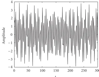
To illustrate the above theorem, suppose that we have a sinu-soidal signal composed of three different frequency compo-nents as shown inFigure 1:
Xt=sin(0.45t)+2∗sin(1.5t)+cos(2.8t), t=1, 2,. . ., 300. (45)
If we perform the cubic spline filtering at scale 0 (without smoothing) and then take the difference up to order 9 or the wavelets with vanishing moments from 1 to 9 in (2).Table 1
shows the zero-crossing counts and the frequency estimates by usingπE(ZC#(W(j)))/(N−1) as in (43).
0 50 100 150 200 250 300
−4
−3
−2
−1 0 1 2 3 4
t
A
m
plitude
Figure1: Supposition of three sinusoids with angular frequencies 0.45, 1.5, and 2.8.
We see that with the increase of differential order, the highest frequency component can be estimated, as proven in
Theorem 3. The middle frequency 1.5 can be estimated by the first- and second-order derivatives.
If we want to estimate the lowest frequency component, according toTheorem 2, we should perform smoothing or take the wavelet transform at higher scales.Table 2provides the results for the wavelet transform at scale 1–9.
The theorems inSection 4also suggest that a combina-tion of smoothing and derivatives can be used to estimate certain frequencies between the lowest and highest frequency components. As an example, we look at the frequency esti-mates at smoothing scales 5 and 10, and the derivatives from 1 to 9 in Table 3. It can be seen that at lower derivatives, we obtain the estimates of lower frequencies. With the in-crease of the order of derivatives, the frequency 1.5 can be estimated.
5.2. Example 2
We look at another example. In this example, the previous signal is added with white noise with variance 2,
Xt=sin(0.45t) + 2∗sin(1.5t) + cos(2.8t) +wn(t), t=1, 2,. . ., 300.
(46)
This signal is plotted inFigure 2.
Table 4shows the frequency estimates for the cases when the vanishing moments of wavelets go from 1 to 9.
Table 5shows the frequency estimates for the cases when the smoothing scales vary from 1 to 9. With the smoothing, the noise is weakened, and so the lowest frequency can be computed.
If we perform the smoothing at scale 5 and then take the wavelets up to the order of 9 , we are able to estimate the frequency components between the lowest and highest ones.
Table1: Zero-crossing counts and frequency estimates.
Derivative orderj 1 2 3 4 5 6 7 8 9
ZC#W1(j)X
138 140 190 229 247 255 259 259 259
ω 1.4950 1.5166 2.0583 2.4808 2.6758 2.7624 2.8058 2.8058 2.8058
Table2: Zero-crossing counts and frequency estimates.
Smoothing scale 1 2 3 4 5 6 7 8 9
ZC#(SjX) 138 130 55 47 42 42 42 41 41
ω 1.4946 1.4083 0.5958 0.5092 0.4550 0.4550 0.4550 0.4442 0.4442
Table3: Frequency estimation at smoothing scales 5 and 10 when the wavelets have vanishing moments from 1 to 9.
Derivative order 1 2 3 4 5 6 7 8 9
ZC#W5(j)X
42 41 120 138 138 139 139 138 138
ω 0.4550 0.4442 1.3000 1.4950 1.4950 1.5058 1.5058 1.4950 1.4950
ZC#(W10(j)X) 41 41 42 41 58 138 138 138 138
ω 0.4442 0.4442 0.4550 0.4442 0.6283 1.4950 1.4950 1.4950 1.4950
0 50 100 150 200 250 300
−6
−4
−2 0 2 4 6
A
m
plitude
t
Figure2: The sinusoidal signal mixed with white noise.
If we take the vanishing moments of the wavelet to be infinite, according toTheorem 3, it will approximate to the highest frequency of the signal. In such an example, it will be
πbecause the spectrum of white noise is from 0 toπ.Table 7
verifies that the highest frequency isπ when the vanishing moments of wavelets go up to 118.
5.3. Example 3
We test Corollary 3by a simple example. Suppose that we have a sinusoidal signal
Xt=sin(0.45t) (47) with frequency 0.45, as plotted inFigure 3.
We consider the cubic-spline wavelet transform with up to 10 vanishing moments or with the 1st–10th-order diff er-ence of cubic-spline filtering. For each wavelet transform,
we present the zero-crossing number counts and the corre-sponding frequency estimates using formula (43). As shown inTable 8, the zero-crossing number remains unchanged ex-cept for numerical errors and the frequency is approximately estimated.
If we perform the spline wavelet filtering at different scales and followed by the same operations described above, the results are shown inTable 9. Due to smoothing, the low frequency components are smoothed out and the estimation becomes inaccurate for higher derivatives.
6. DISCUSSIONS
In this paper, we have investigated how the number count-ing of zero crosscount-ings of a wavelet transform can be used to estimate the frequency components of signals in a fast and simplistic fashion. It is well known that the FFT is the most commonly used tool to estimate a signal’s spectrum, with a computational complexity ofO(NlogN), whereN is the length of the signal. Under the approach proposed in this pa-per, the computation of differential wavelet transforms and ((19), (20), and (21)) can in fact all be implemented with additions only. The complexity associated with such an ap-proach is simply linear, and therefore much lower than that of the FFT approach. The estimation of signal frequency has also been investigated in [19], where a continuous Gabor-based wavelet transform was used. However this latter ap-proach appears to be computationally much more demand-ing because of the need to compute the continuous wavelet transform.
Table4: Frequency estimation for the signal mixed with white noise using wavelets with vanishing moments up to 9.
Derivative order 1 2 3 4 5 6 7 8 9
ZC#W1(j)X
183 195 213 235 236 243 245 255 258
ω 1.9825 2.1125 2.3074 2.5458 2.5566 2.6324 2.6541 2.7624 2.7949
Table5: Frequency estimation for the signal mixed with white noise using a smoothing scale from 1 to 9.
Smoothing scale 1 2 3 4 5 6 7 8 9
ZC#W1 sX
92 64 54 48 46 44 42 38 37
ω 0.9699 0.6747 0.5692 0.5060 0.4849 0.4639 0.4428 0.4006 0.3901
Table6: The smoothing and derivative operations can be combined to estimate certain frequencies in between the lowest and highest frequency.
Derivative order 1 2 3 4 5 6 7 8 9
ZC#W5(j)X
39 62 85 121 138 140 142 141 144
ω 0.4084 0.6493 0.8901 1.2671 1.4451 1.4661 1.4870 1.4765 1.5080
Table7: Frequency estimation for the signal mixed with white noise using wavelets when the vanishing moments are larger than 115.
Derivative order 115 116 117 118 119 120 121 122 123
ZC#W1(j)X
37 37 37 39 39 39 39 39 39
ω 2.9805 2.9805 2.9805 3.1416 3.1416 3.1416 3.1416 3.1416 3.1416
0 50 100 150 200 250 300
−1
−0.8
−0.6
−0.4
−0.2 0 0.2 0.4 0.6 0.8 1
A
m
plitude
t
Figure3: A sinusoidal signal.
In this work, we show that the zero crossings in the diff er-ential spline wavelet domain can be used to effectively ap-proximate the frequencies of a signal. Higher frequency can be estimated by wavelets with higher order of vanishing mo-ments, while lower frequency can be estimated by increasing the smoothing scale. Proper use of the smoothing scale and differential order can facilitate the estimation of certain fre-quency components. The relationship between the wavelet transform signatures of a signal and its frequency estimation based on Fourier transform is thus established. Formula (27) also offers a way to compute the autocorrelation, which is of-ten used in signal spectrum analysis [2,3,21].
In the scale-space theory for computer vision, the zero crossings in multiscale or scale-space filtering are usually re-ferred to as the fingerprints in the scale-space theory [22,23]. The famous scaling theorem states that the Gaussian kernel is the only filter with which the number of zero crossings of a signal does not increase with the increase of the smoothing scale [24]. This property is also known as the monotone or the embedding property that has been proven for the con-tinuous signal case. In practice, however, the kernels used for scale-space filtering are not Gaussian. For example, some of the most commonly used kernels are spline approximations [8,25], or more general scaling filters in the wavelet theory [26]. It has been shown that for discrete signals, the above embedding property still holds for certain discrete smooth-ing kernels [27]. Whether the embedding property still holds for more general discrete smoothing filters, in particular the spline filters, has not been proven previously. The results pre-sented in this paper attempt to provide a rigorous proof of this property for a random signal in the discrete setting.
ACKNOWLEDGMENTS
Table8: Frequency estimation for the sinusoidal signal.
Derivative order 1 2 3 4 5 6 7 8 9
ZC#W1(j)X
41 42 41 42 41 42 41 41 42
ω 0.4442 0.4550 0.4442 0.4550 0.4442 0.4550 0.4442 0.4442 0.4550
Table9: The effect of smoothing on the estimation of the pure sinusoidal signal.
Derivative order 1 2 3 4 5 6 7 8 9
ZC#W5(j)X
43 42 43 44 44 44 44 44 48
ω 0.4503 0.4398 0.4503 0.4608 0.4608 0.4608 0.4608 0.4608 0.5027
REFERENCES
[1] B. Kedem, “Spectral analysis and discrimination by zero-crossings,”Proc. IEEE, vol. 74, no. 11, pp. 1477–1493, 1986. [2] N. Rudhakrishnan, J. Wilson, C. Lowery, H. Eswaran, and
P. Murphy, “A fast algorithm for detecting contractions in uterine electromyography,” IEEE Eng. Med. Biol. Mag., vol. 19, no. 2, pp. 89–94, 2000.
[3] L. J. Hadjileontiadis, “Discrimination analysis of discontinu-ous breath sounds using higher-order crossings,”IEE Medical & Biological Engineering & Computing, vol. 41, no. 4, pp. 445– 455, 2003.
[4] R. M. Haralick, “Digital step edges from zero crossing of sec-ond directional derivatives,” IEEE Trans. Pattern Anal. Ma-chine Intell., vol. 6, no. 1, pp. 58–68, 1984.
[5] S. Mallat, “Zero-crossings of a wavelet transform,” IEEE Trans. Inform. Theory, vol. 37, no. 4, pp. 1019–1033, 1991. [6] N. Saito and G. Beylkin, “Multiresolution representations
using the autocorrelation functions of compactly supported wavelets,” IEEE Trans. Signal Processing, vol. 41, no. 12, pp. 3584–3590, 1993.
[7] Y.-P. Wang, “Image representations using multiscale differen-tial operators,”IEEE Trans. Image Processing, vol. 8, no. 12, pp. 1757–1771, 1999.
[8] Y.-P. Wang and S. L. Lee, “Scale-space derived from B-splines,” IEEE Trans. Pattern Anal. Machine Intell., vol. 20, no. 10, pp. 1040–1055, 1998.
[9] B. Kedem, “On the sinusoidal limit of stationary time series,” Ann. Stat., vol. 12, no. 2, pp. 665–674, 1984.
[10] E. Suhir,Applied Probability for Engineers and Scientists, chap-ter 8, McGraw-Hill, New York, NY, USA, 1997.
[11] P. Flandrin, “Wavelet analysis and synthesis of fractional Brownian motion,” IEEE Trans. Inform. Theory, vol. 38, no. 2, pp. 910–917, 1992.
[12] Y.-P. Wang, S. L. Lee, and K. Torachi, “Multiscale curvature based shape representation using B-spline wavelets,” IEEE Trans. Image Processing, vol. 8, no. 11, pp. 1586–1592, 1999. [13] S. O. Rice, “Mathematical analysis of random noise,” Bell
System Technical Journal, vol. 24, pp. 46–156, 1945.
[14] B. Kedem, “A stochastic characterization of the sine function,” J. Amer. Math. Monthly, vol. 93, no. 6, pp. 430–440, 1986. [15] B. Kedem, , and T. Li, “Monotone gain, first-order
autocor-relation, and expected zero-crossing rate,” Ann. Stat., vol. 19, pp. 1672–1676, 1991.
[16] M. B. Priestly, Spectral Analysis and Time Series, Academic Press, New York, NY, USA, 1981.
[17] R. G. Laha and V. K. Rohatgi,Probability Theory, John Wiley, New York, NY, USA, 1979.
[18] Z. Bai, C. R. Rao, Y. Wu, M.-M. Zen, and L. Zhao, “The simul-taneous estimation of the number of signals and frequencies
of multiple sinusoids when some observations are missing: I. Asymptotics,” Proc. Natl. Acad. Sci. USA, vol. 96, no. 20, pp. 11106–11110, 1999.
[19] N. Delprat, B. Escudi´e, P. Guillemain, R. Kronland-Martinet, P. Tchamitchian, and B. Torr´esani, “Asymptotic wavelet and gabor analysis: extraction of instantaneous frequencies,”IEEE Trans. Inform. Theory, vol. 38, no. 2, pp. 644–664, 1992. [20] B. Logan, “Information in the zero crossings of bandpass
sig-nals,”Bell System Technical Journal, vol. 56, no. 4, pp. 487–510, 1977.
[21] R. E. Passarelli Jr. and A. Siggia, “The autocorrelation func-tion and spectral moments: geometric and asymptotic inter-pretations,”J. Clim. Appl. Meteorol., vol. 22, no. 22, pp. 1776– 1787, 1983.
[22] B. M. ter Haar Romeny, L. Florack, J. J. Koenderink, and M. A. Viergever, Eds., Scale-Space Theory in Computer Vision, First International Conference, Scale-Space ’97, Utrecht, The Nether-lands, vol. 1252 ofLecture Notes in Computer Science, Springer, Berlin, Germany, 1997.
[23] T. Lindeberg, “Scale-space theory: a basic tool for analysing structures at different scales,”J. Appl. Statist., vol. 21, no. 2, pp. 224–270, 1994, (Supplement on Advances in Applied Statis-tics: Statistics and Images: 2).
[24] A. L. Yuille and T. Poggio, “Scaling theorems for zero-crossings,” IEEE Trans. Pattern Anal. Machine Intell., vol. 8, no. 1, pp. 15–25, 1986.
[25] M. Unser, A. Aldroubi, and M. Eden, “TheL2-polynomial spline pyramid,” IEEE Trans. Pattern Anal. Machine Intell., vol. 15, no. 4, pp. 364–379, 1993.
[26] I. Daubechies,Ten Lectures on Wavelets, Society for Industrial and Applied Mathematics, Philadelphia, Pa, USA, 1992. [27] T. Lindeberg, “Scale-space for discrete signals,” IEEE Trans.
Pattern Anal. Machine Intell., vol. 12, no. 3, pp. 234–254, 1990.
Jie Chenreceived the B.S. degree in applied mathematics from Chongqing University, Chongqing, China, in 1985, the M.S. de-gree in applied statistics from University of Akron, Akron, Ohio, in 1990, and the Ph.D. degree in statistics from Bowling Green State University, Bowling Green, Ohio, in 1995. She is currently an Asso-ciate Professor of statistics in the Department of Mathematics and Statistics, University of Missouri-Kansas City, Kansas City, Mo. Her research interests are in the areas of change-point analysis, model selection criteria, applied statistics, multivariate statistical analysis, and microarray gene expression modeling. She is the Coauthor of the bookParametric Statistical Change Point Analysis(Birkh¨auser, Boston, 2000).
Qiang Wureceived the Ph.D. degree in elec-trical engineering in 1991 from the Catholic University of Leuven (Katholieke Univer-siteit Leuven), Belgium. In December 1991, he joined Perceptive Scientific Instruments, Inc., Houston, Tex, where he was a Senior Software Engineer from 1991 to 1994, and was a Senior Research Engineer from 1995 to 2000. He was a key contributor to the research and development of the core
tech-nologies for PSI’s automated microscopy products for cytogenetics applications, including digital microscope autofocusing and imag-ing, image segmentation, enhancement, recognition, and compres-sion for automated chromosome karyotyping, and fluorescence in situ hybridization (FISH) image analysis for automated assessment of low-dose radiation to NASA astronauts during space missions. He is currently a Lead Research Engineer at Advanced Digital Imag-ing Research, LLC, Houston, Tex. He has served as a Principal In-vestigator on numerous National Institutes of Health (NIH) re-search grants. His rere-search interests include image processing, pat-tern recognition, artificial intelligence, and their biomedical appli-cations.
Kenneth R. Castleman is the noted au-thor of the seminal textbook Digital Im-age Processing. After earning his B.S., M.S., and Ph.D. degrees in electrical and biomed-ical engineering, all from the University of Texas, Dr. Castleman went to work for NASA’s Jet Propulsion Laboratory. In 1984, he cofounded Perceptive Systems Inc. (PSI), and began commercializing digital imaging technology. He is currently the President of