R E S E A R C H
Open Access
Efficiency improvement in multi-sensor wireless
network based estimation algorithms for
distributed parameter systems with application
at the heat transfer
Constantin Volosencu
*and Daniel-Ioan Curiac
Abstract
This paper gives a technical solution to improve the efficiency in multi-sensor wireless network based estimation for distributed parameter systems. A complex structure based on some estimation algorithms, with regression and autoregression, implemented using linear estimators, neural estimators and ANFIS estimators, is developed for this purpose. The three kinds of estimators are working with precision on different parts of the phenomenon
characteristic. A comparative study of three methods - linear and nonlinear based on neural networks and adaptive neuro-fuzzy inference system - to implement these algorithms is made. The intelligent wireless sensor networks are taken in consideration as an efficient tool for measurement, data acquisition and communication. They are seen as a“distributed sensor”, placed in the desired positions in the measuring field. The algorithms are based on
regression using values from adjacent and also on auto-regression using past values from the same sensor. A modelling and simulation for a case study is presented. The quality of estimation is validated using a quadratic criterion. A practical implementation is made using virtual instrumentation. Applications of this complex estimation system are in fault detection and diagnosis of distributed parameter systems and discovery of malicious nodes in wireless sensor networks.
Keywords:Intelligent sensor networks, Distributed parameter systems, Estimation techniques, System monitoring, Virtual instrumentation
1. Introduction
The paper presents some theoretical and practical aspects of signal processing in the new and emerging technology of wireless sensor networks. The application is directed to the practicing engineers and also to the academic researchers. The problem covered in this paper is in the area of algorithms of multivariable estimation, architec-ture of system dedicated to process monitoring based on smart sensor and system implementation. The practical applications of this paper could be processes seen as dis-tributed parameter systems. Advances in hardware and wireless network technologies have created smart, low-cost, low-power, multifunctional miniature sensor devices.
The sensor number in a network is over hundreds or thousands of ad hoc tiny sensor nodes spread across dif-ferent areas. Thus, the network actively participates in cre-ating a smart environment. They are low cost and low energy devices, realized in nanotechnology. With them we may develop low cost wireless platforms, including inte-grated radio and microprocessors. These devices make up hundreds or thousands of ad hoc tiny sensor nodes spread across a geographical area. These sensor nodes collaborate among themselves to establish a smart sensing network. A sensor network can provide access to information any-time, anywhere by collecting, processing, analyzing and disseminating data. Wireless sensor networks are ex-tremely distributed systems having a large number of in-dependent and interconnected sensor nodes, with limited computational and communicative potential. The sensors are deployed for data acquisition purposes in a wide range
* Correspondence:[email protected]
Faculty of Automatics and Computers, Department of Automatics and Applied Informatics,“Politehnica”University of Timişoara, Bd. V. Parvan nr. 2, Timisoara 300223, Romania
of locations, sometimes in resource-limited and hostile environments such as disaster areas, seismic zones, eco-logical contamination sites and other different zones. This structure has the following characteristics: data processing is at the sensor level, data transmission is wireless, the sensing mechanism does not need more power supply. Sensor network applications include: environmental mon-itoring, civil infrastructure monmon-itoring, shared resource utilization, tracking, perimeter protection and surveil-lance. Applications are in micro-climates, air quality, soil moisture, animal tracking, energy usage, office comfort, wireless thermostats, wireless light switches. In techniques they have applications such as data acquisition of physical and chemical properties, at various spatial and temporal scales, distributed parameter systems, for automatic iden-tification, measurements over a long period of time. The modern sensors are smart, small, lightweight and portable devices, with a communication infrastructure intended to monitor and record specific parameters like temperature, humidity, pressure, wind direction and speed, illumination intensity, vibration intensity, sound intensity, power-line voltage, chemical concentrations and pollutant levels in diverse locations. The sensor networks are deployed for data acquisition purposes in a wide range of locations, in resource-limited and hostile environments such as disaster areas, seismic zones, contaminated ecological sites and so on. All these applications are distributed parameter sys-tems. The nature of wireless sensor networks as smart and small distributed sensors could be of interest in a large class of smart and autonomous applications, capable to be implemented in multiple processes seen as largely distributed parameter processes. Also, the identification and malicious node detection in a distributed parameter system depends on sensor network interfacing with the real world. The sensors are adequate for autonomous operation in highly dynamic environments as distributed parameter systems. We may add sensors when they fail. They require distributed computation and communica-tion protocols. They assure scalability, where the quality can be traded for system lifetime. They assure Internet
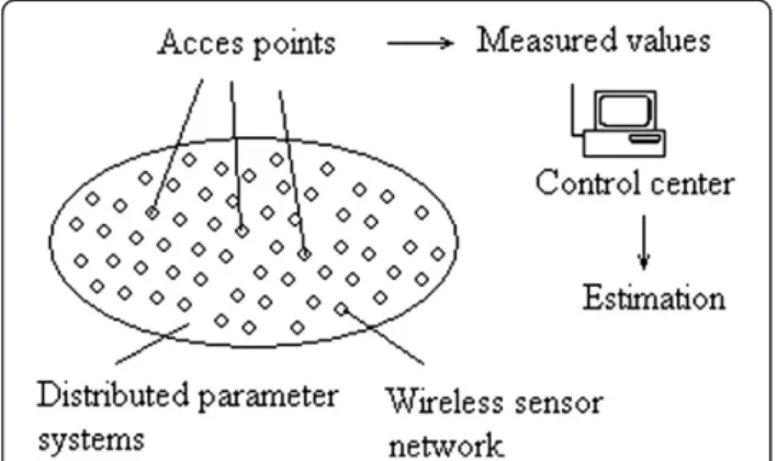
connections via satellite. Based on the above consider-ation we may say: the intelligent sensor networks may be seen as a “distributed sensor” placed in the field of a distributed parameter system.
The paper presents the results of applied research and application of sensor networks as a new emerging type of “distributed sensor” for physical variables in engineering problems. These kinds of applications are adequate for estimation, monitoring, fault detection and diagnosis in distributed parameter systems. This application is framed in the field of industrial pro-cesses or environment systems which may be seen as distributed parameter systems. A distributed sensor
network may be seen in this case as a ”distributed”
sensor placed into the field of a distributed parameter system. Examples of distributed parameter systems with large application in practice are: the process of heat conduction, applications related to the field of electricity, motion of fluids, the processes of cooling and drying, the phenomenon of diffusion and other applications are presented. The variables of these pro-cesses are: temperature, pressure, humidity, acceler-ation and so on. All of them may be measured with wireless sensor networks. The estimation made using sensor networks is useful for applications ranging from control systems, fault detection and diagnosis, signal processing to time-series analysis. In theory there are methods to estimate linear black box models and models of artificial intelligence for non-linear systems. Also, an important application may be the malicious node detection in wireless sensors, based on such esti-mation techniques. The data are input from sensors into automate systems using virtual instrumentation and adequate drivers.
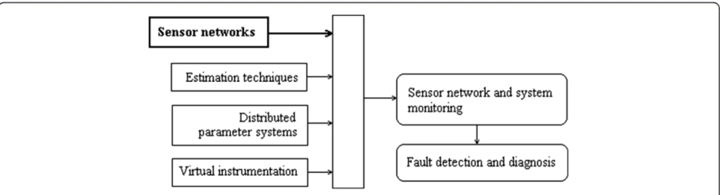
The novelty value of this paper consists in applying some concepts such as sensor networks as a“distributed sensor”, estimation techniques and virtual instrumenta-tion to distributed parameter systems, with many appli-cations in practice, such as system monitoring for fault detection and diagnosis, as it is illustrated in Figure 1.
Some simplifying methods for modelling these sys-tems, that are trying to capture the distributed system dynamics through lumped parameter models, are used. The estimation equations were developed for estimator based on regression and auto-regression, with linear and non-linear models based on neural networks and adap-tive neuro-fuzzy inference systems (ANFIS). A case study for the heat transfer, based on auto-regression esti-mator equation, is presented. Some modelling and simu-lation results are presented. The estimation results were compared based on the quadratic error criterion. For practical purposes a virtual instrument was built and tested for monitoring sensor networks, including the es-timation. Based on the estimates, errors and faults in sensor network and of course in the field of distributed parameter systems, may be detected. A technical contri-bution based on multivariable estimation techniques, distributed parameter system theory and virtual instru-mentation is presented with consistency. Starting from three standard methods to implement the novel estima-tion algorithms based on sensor networks for distributed parameter systems, in the discretized version of them, we are showing what is the better method to increase the quality of estimation, related to the complexity of im-plementation. The role of the sensor network is a major one, because it is seen as a distributed sensor placed in the field. All the critical aspects which are arising in identifica-tion of distributed parameter systems from large data are taken into consideration: the structure of the estimator is determined, an adequate variable selection is made and last but not least the distributed computation is solved using the distributed intelligent sensor placed into a net-work with a collecting base station. There is a substantial and structured overview of references in the chapter of related work, focused on the problem. The paper starts from the classical model of the parabolic distributed par-ameter systems, which are presented in an implicit form, then in an explicit form.
The main contribution of this paper is a complex esti-mation structure, resulted using combined two estiesti-mation algorithms, with regression and auto-regression, devel-oped in other papers, implemented using three efficient estimation methods: one linear and two non-linear - with neural networks and ANFIS. This complex system is used
to estimate the value of the sensor at the moment t+1,
based on the past values of the same sensor and also based on the current values of the adjacent sensors. One of the estimation algorithms is using the values of the adjacent sensors and the other algorithm is using the antecedent values of the same sensor. A discrete approximation of parabolic models and the two estimation algorithms pre-sented in the paper have already tested on different case studies, and the results were been published by the authors in references [1,2,3,4]. A short consideration is
made on this knowledge, with simple equations, offered to understand how the complex estimator works. From the explicit form of the equation, which is a more general form of the distributed parameter system, the possible order of the estimator is determined, the variables are selected, and two computation algorithms are presented. Following these considerations the model structure imposed by the distributed parameter system dynamics is modelled into the estimation algorithms. The meshes in the distributed system are a good indication how to place the sensors in the field. The neural estimator was previ-ously tested on some case studies, and the results were presented in [5]. The ANFIS estimator was tested on some case studies, and the results were presented in [3]. The ANFIS estimator with the estimation algorithms were tested on a practical application in environmental moni-toring and the results were presented in [4].
The intelligent sensor network with its base station, the PC drivers and the virtual instrumentation solved
the problem of the associated constrains–
communica-tion, computation and so on. The practical contribution of this paper is that it presents how to improve the esti-mation quality in the case of an estiesti-mation using sensor networks, in a real time application, for fault detection and diagnosis.
2. Related work
Since for distributed parameter systems it is impossible to observe their states over the entire spatial domain, a pos-sible solution is to locate discrete sensors to estimate the unknown system parameters as accurately as possible. There is recent original work on optimal sensor placement strategies for parameter identification in dynamic distribu-ted systems modeled by partial differential equations. The development of new techniques and algorithms or adopting methods, which have been successful in the field of optimal control and optimum experimental design, is reported in different papers. Advances in scientific computation and developments in spatial sensor technology have enhanced the ability to develop modelling strategies and experimental techniques for the study of the space-temporal response of distributed non-linear systems. Robust implementations of distributed system identification algorithms based on detailed space and time experimental data have an import-ant role in practical applications. Wireless automation is today an emerging topic.
by introducing the concepts of interconnection matrices, system digraphs, and cut point sets, real-time field estima-tion algorithms are derived. Simulaestima-tions and real world experiments on temperature estimation are conducted.
A strategy by which sensor nodes detect and estimate non-localized phenomena such as boundaries and edges (e.g., temperature gradients, variations in illumination or contamination levels) can be found in study [13]. A gen-eral class of boundaries, with mild regularity assumptions, is considered, and a theory on the achievable performance of sensor network based boundary estimation is estab-lished. A hierarchical boundary estimation algorithm is proposed that achieves a near-optimal balance between mean-squared error and energy consumption.
In the paper [14] the state of the art algorithms for consensus-based distributed estimation using ad hoc wire-less sensor networks, where sensors communicate over single-hop noisy links, are presented. Basic estimation cri-teria such as least-squares, maximum-likelihood and others are reformulated in a novel framework, amenable to dis-tributed solutions. The framework encompasses adaptive filtering and smoothing of non-stationary signals through distributed LMS and Kalman filtering.
The functions of different wireless technologies are described in [15,16]. In the survey paper for system identi-fication [17] it is shown that the sensor networks repre-sent“an open area in system identification, being a rapidly evolving technology to collect information with many spatial distributed, autonomous devices. They have an interesting potential for industrial monitoring purposes and add to the richness of information for model
develop-ment.” The development of wireless sensor allows the
application of many methods and algorithms for identifi-cation of systems, with a high efficiency in the particular case of the distributed parameter systems. The main prin-ciples consist in the fact that in this kind of identification the sensor network may be seen as a“distributed sensor” placed into a field, which is a distributed parameter sys-tem, allowing measurement in well-chosen points of an infinite variable system. In the emerging area of research in wireless sensor network the applications paper [18] pre-sents the design of a wireless network sensor, based on a database, which archives the data reported by distributed sensors, as well as the implemented support for queries and data presentation. In the paper [19] an architecture of a set of mobile sensors is developed were the sensors col-laborate with the stationary sensors in order to detect an event, for an accurate view of the state of the environ-ment. The special issue [20] brings together contributions from signal processing, communications and new algo-rithm design methodologies of cooperative localization systems. An application of wireless sensor networks for RF-based indoor localization is presented in [21]. In the special issue [22] the state of the art and emerging
distributed signal processing techniques in wireless sensor networks, are presented, estimation being one of them. In the special issue [23] the recent interest in develop-ing sensor networks for different sensible applications, for area monitoring, including detecting, identifying, lo-cating and tracking the emission signals of interest is emphasized. The special issue [24] deals with various signal processing aspects of sensor networking, which are significant for providing measurements of the phys-ical phenomenon around, for understanding and using this information in a wide range of potential applica-tions including environmental monitoring, health care monitoring, harsh field surveillance and reconnais-sance, modern manufacturing, condition based main-tenance of complex systems, and so forth.
For sensor network monitoring there are different technical solutions. In the paper [25] a software environ-ment for monitoring and controlling sensor network via a web interface is presented.
Some recent applications of sensor networks in which distributed parameter process monitoring is of interest are presented as follows. Thus, a possible application of sensor networks, in a field with distributed points, is the tracking problem of a dynamic object movement be-tween these distributed points on the field. The paper [26] presents a technical solution based on acoustic and visual sensors. Another solution for real time tracking in wireless sensor networks is presented in the paper [27]. The usage of estimation for monitoring service attacks in sensor networks is an important application. A tech-nical solution for solving this problem using algorithms for filtering bogus signals from different sensors from the field is presented in the paper [28]. An example of industrial process application in manufacturing plasma treatment for polymers is presented in the paper [29].
Some papers in which the sensor networks are used for estimation purposes are [30], where a graph ap-proach is presented, and [31], where for estimation reduced order physical models are used.
distributed systems by large-scale collaborative sensor networks is initiated, based on the distributed Karhunen-Loève transformation. The reduction of the distortions at the nodes and the low computational complexity of the fusion algorithm at the fusion centre are taken into con-sideration. The algorithm is applied on a system described by a partial differential equation in 2-D domain. A state estimation problem is considered in the paper [34], based on a Kalman filter, in which two communication schemes are producing estimates at the fusion centre. Some simu-lations are provided, under various circumstances. The paper [35] presents an application of sensor networks for distributed H∞ consensus filtering with multiple missing
measurements. The identification of non-linear systems continues to be a contemporary problem, trying to be solved using different methods, for example in [36] for un-known nonlinear system, given the distribution knowledge of the system inputs. Artificial neural networks have seen significant applications over the last decades in the area of system identification, as a flexible way to give hyper-surfaces for regression, being very effective for solving a large number of non-linear estimation problems [17]. The paper [37] treats an application of partial differential equa-tions, considering that neural networks can approximate a large set of continuous functions defined on a compact set to an arbitrary accuracy. The paper [9] presents an appli-cation of unsupervised regression at non-linear system identification. An approximation algorithm for optimising a cost function is developed, as manifold learning using low dimensional coordinates. ANFIS is a well-known method for development self-organizing neuro-fuzzy sys-tems with many applications in practice. After years of try-ing to find new algorithms, ANFIS is still in use, and recent applications were reported such as [38] or an appli-cation of ANFIS at sensor data processing [39] or [11]. The paper [26] presents some aspects related to the esti-mation of average air temperature in the built environ-ment by using integer neural networks, ANFIS and inferential sensor models. The paper compares the results of these models, presenting their advantages and disad-vantages. Time series predictions based on ANFIS are pre-sented in the literature, for example [40]. Applications of fault detection and diagnosis in distributed parameter sys-tems are presented as follows. In the paper [14] the prob-lem of fault detection in distributed parameter systems is formulated as maximizing the power of a parameter hy-pothesis testing whether the system parameters have nom-inal values or not. The sensor locations are given a priori. A gradient projection algorithm is proposed to perform the search for the optimal solution. The approach is illu-strated by a numerical example for a two-dimensional dif-fusion process. The paper [41] considers the problem of designing fault diagnosis algorithms for dynamic systems
using sensor networks. A network of distributed
estimation agents is designed, with local Kalman filter em-bedded into each sensor. The diagnosis decision is per-formed by a distributed hypothesis testing method that relies on a belief consensus algorithm. Simulation results are provided to demonstrate the effectiveness of the pro-posed architecture and algorithm.
3. General mathematical model of the parabolic distributed parameter system with application at the heat transfer
The distributed parameter systems have general math-ematical models in continuous time and space as partial differential equation, of parabolic form, as:
∂θ
∂t ¼c1∇ðc2∇θÞ þc3θþQ ð1Þ where the variables θ(ζ, t) depend on time t≥0 and on space ζ∈V, where ζ is x for one axis and (x, y) for two axis, c1, c2 and c3 are coefficients, which could be also time variant andQ(ζ, t) is an exterior excitation, variable on time and space. So, in the general case, an implicit equation may be written:
f ∂θ
∂t;
∂θ
∂ζ;
∂2θ ∂ζ2;. . .
¼0 ð2Þ
For the partial differential equation (1) some boundary conditions may be imposed to establish a solution. So, when the variable value of the boundary is specified there are Dirichlet conditions:
c4θ¼q ð3Þ
and, when the variable flux and transfer coefficient are specified there are Neumann conditions:
c5∇θþc6θ¼0 ð4Þ
In the practical application case studies limits and ini-tial conditions of the equation (1) are imposed:
θð0;tÞ ¼θζ0; t∈½0;T;θ ζð ;0Þ ¼0;ζ∈½ 0;l;
θð Þ ¼l;t θζl;t∈½0;T ð5Þ
A system with finite differences may be associated with the equation (1). For this purpose the space S is divided into small pieces of dimensionlp:
lp¼l=n ð6Þ
In each small piece Spi, i=1,. . .,n of the space S the
variable θ could be measured at each moment tk, using
time, and derivatives of first and second order in space. So, theoretically, we may approximate the variable deri-vatives in time with small variations in time, with the following relation:
∂θ
∂t ¼ θkþ1
i θ k i
tkþ1tk ; ð
7Þ
The first and the second derivatives in space may be approximated with small variations in space to obtain the following relations. For the x-axis we may write the following equations:
∂θ
∂x¼ θk
i θ k i1
lp ;
∂2θ ∂x2¼
θk
iþ12θki þθki1
l2
p
ð8Þ
The same equations may be written also for theyaxis. Of course, an equation with variables written in vectors could be written. We may consider the variable is mea-sured as sampleθik=θ(ζi,tk),ζi∈V, at equal time intervals with the value:
h¼tkþ1tk ð9Þ
called sample period, in a sampling procedure, with a
digital equipment, at the sample time moments tk=kh.
For the parabolic equation a linear approximate system of derivative equations of first degree may be used:
dΨ
dt ¼AΨþBQ ð10Þ
where, this time, ψ is a vector containing the values of the variableθ(ζ, t) in different points of the space and at different moments in time.
Combining the equations (7, 8) in the equation (1) a system of equations with differences results for the para-bolic equation [1,3,4]:
fp θki;θki1;θkiþ1;θkiþ1
¼0 ð11Þ
Several estimation algorithms may be developed as fol-lows, based on the discrete models of the partial deriva-tive equations, taking account of the equations (11).
4. Multisensor network based estimation algorithms and monitoring method 4.1 Estimation algorithms
Analysing the form of the equation (11) we may see a number n=4 of variables involved: θik,θik−1,θik+1,θik+1, which are the measured variables from the sensors placed in 3 adjacent points Pi-1(ζi-1), Pi(ζi) and Pi+1(ζi), i=1,. . .,n of the space S, at two moments: tk and tk+1. Based on the structure of the equation (11) we may de-velop estimation algorithms using the values measured at 3 adjacent sensors: θik−1,θik+1,θik or using the
ante-cedent values of the same sensor: θik,θik−1,θik−2,θik−3.
These novel estimation algorithms, which are developed for multisensor networks are presented as follows [1,3,4].
Estimation algorithm 1. It estimates the value of the variable θik+1 at the moment tk+1, measuring the values of the variables θik−1,θik+1,θik at the antecedent moment
tk:
θkþ1
i ¼f1 θki1;θkiþ1;θki
ð12Þ
This is a multivariable estimation algorithm, based on adjacent points in space (nodes or sensors).
Estimation algorithm 2. It estimates the value of the variable θik+1 at the moment tk+1, measuring the values of the same variableθik,θik−1,θik−2,θik−3, but at four
anter-ior momentstk,tk-1,tk-2andtk-3.
θkþ1
i ¼f2 θki;θik1;θki2;θki3
ð13Þ
The estimator could be a linear or a non-linear one, described by the function y=f(u1, u2, . . ., un), using dif-ferent estimator implementation methods. In this paper three estimator implementation methods are used and compared: a linear estimator, an estimator based on a feedforward neural network with continuous values and an estimator based on an ANFIS. The number of inputs depends on the estimation algorithm, on the specific position in space of the measuring points, and on the conditions of determination.
4.2 Monitoring method
The defined distributed system in the practical applica-tion is the process of heat distribuapplica-tion, in the real world. The following method is according to the objectives of monitoring of this real process. These systems have known mathematical model as a parabolic partial differ-ential equation as a primary model from physics, with well-defined boundary and initial conditions for the sys-tem in practice. These represent the basic knowledge for a reference model from real data observation. The pri-mary physical model must be discretized, to obtain a mathematical model as a MIMO state-space model. The unstructured meshes may be generated.
In the field of the distributed parameter system several sensors are placed, as it is presented in Figure 2.
For each point PA there is a sensor SA and around it there are other 4 adjacent points Padj1, Padj2, Padj3 and Padj4in which there are placed 4 sensors Sadj1, Sadj2, Sadj3 and Sadj4, like in Figure 3.
The sensor network, made by hundreds of ad-hoc tiny sensor nodes is spread across the space. Sensor nodes collaborate among themselves, and the sensor network provides information anytime, by collecting, processing, analyzing and disseminating temperature measured data. New nodes are automatically detected and incorporated. The number and the place point of the de sensor nodes may be discussed according to the desired accuracy of estimation. A scenario for practical applications could be chosen and simulated. The simulation and the practical measurements are producing transient regime character-istics. Those transient characteristics are due to the sys-tem dynamics in a training process. In a steady state we cannot obtain an estimator model. On these transient characteristics, seen as times series, the estimation algo-rithms may be applied. Some estimators may be used to
implement the estimation algorithms. With these algo-rithms future states of the process may be estimated. Possible faults in the system are chosen and strategies for detection may be developed, to identify and to diag-nose them, based on the state estimation. In practice ap-plying the method presumes the following steps: -placing a sensor network in the field of the distributed parameter system; -acquiring data, in time, from the sen-sor nodes, for the system variables; -using measured data to determine an estimation model; -using measured data to estimate the future values of the system variables; -im-posing an error threshold for the system variables; -com-paring the measured data with the estimated values; -if the determined error is greater, then a threshold default occurs; -diagnosing the default, based on estimated data, determining its place in the sensor network and in the dis-tributed parameter system field.
Based on this placement of sensors some estimation
algorithms may be developed. For only one sensor SAan
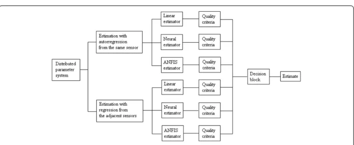
estimation algorithm based on auto-regression of the values acquired from this sensor at several antecedent moments may be used. Using the 4 adjacent sensors an estimation algorithm with regression of the values from these sensors at the same moment may be used. To im-plement these two types of algorithms several estimation functions may be used. One of them may be a linear one. Other two may be non-linear, for example a neural one and an ANFIS one. According to these assumptions, a combination of six algorithms results. The comparison of the algorithms and their results is made by using a quadratic quality criterion. For each algorithm a quality criterion is calculated at each estimation. The decision related to the estimation efficiency is taken into a deci-sion block, using several decideci-sion obtained by reasoning. And the best estimate is provided at the output of this strategy for efficiency improvement.
The estimators are tuned or trained using some study cases adequately chosen for the distributed parameter system.
Figure 2Sensor placed in the field.
Figure 3Adjacent points and sensors.
The structures of the estimators for a study case will be presented in the following part of the paper.
Several quadratic error criteria may be used.
4.3 The complex estimation structure
To increase the efficiency of estimation in a multi-sensor monitoring system dedicated to a distributed par-ameter system the structure from Figure 5 is proposed.
The reason for using three types of estimators is as fol-lows. The process to be estimated has characteristics which are linear, non-linear of a low degree and high non-linear in some parts. The estimators are chosen for each of these three types of characteristics to give the best estimate, with the smallest error: linear estimator, to estimate the linear parts, neural estimator, to estimate parts with a low non-linearity level and ANFIS estimator, to estimate the high level non-linear parts.
5. Methods to implement the estimation algorithms
5.1 Linear estimator
When a linear estimation method is used for implemen-tation the estimator has the following general equation:
y¼a1u1þa2u2þa3u3þa4u4 ð14Þ
where y is the estimate, obtained by using four input
variables u1, u2, u3 and u4 and ai are constant coeffi-cients, obtained by using a least square method. To de-sign the estimators of the isensor, for i=1,. . .,m sensors and points in space, a set ofNmeasured variables, from the sensor networks are required:
xið Þtk ;i¼1;. . .m;k¼1;. . .;N ð15Þ
An error is imposed:
ei;k ¼xið Þ tk xið Þtk ;i¼1;. . .;m; k
¼1;. . .;N ð16Þ
And a quadratic quality criterion, too:
Ji¼
1 2
XN
j¼1
e2i;k; i¼1;. . .;m ð17Þ
The estimator equation is:
xiðtkþ1Þ ¼ai;0xið Þ þtk ai;1xiðtk1Þ þai;2xiðtk2Þþ þai;3xiðtk3Þ;i¼1;. . .;m; k¼3;. . .;N1
ð18Þ
The estimator coefficients are obtained using the least square method:
∂J
∂ai¼
0;i¼0;1;2;3 ð19Þ
Some examples of the linear estimator coefficients obtained for the case study are presented in the paper.
5.2 Neural estimator
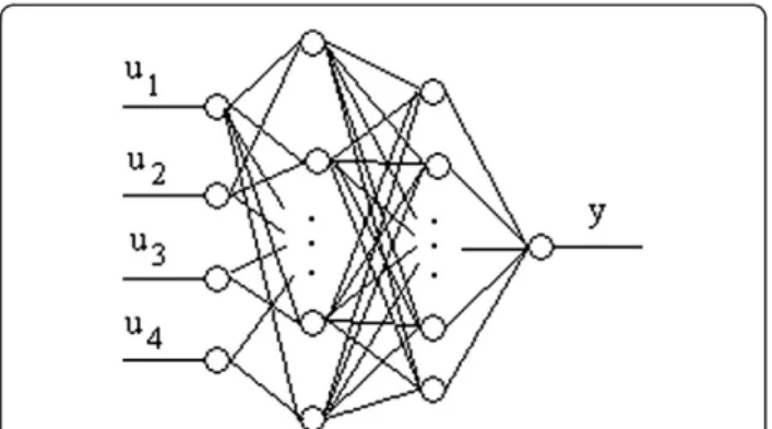
The neural network used for estimation is a feedforward neural network, with continuous values [2]. It has 4 inputs, which may be, for the auto-regression algorithm the sensor values at 4 antecedent moments u1=xA(t-1), u2=xA(t-2), u3=xA(t-3) andu4=xA(t-4), or for the regres-sion algorithm four values of adjacent sensors at the same time moment u1=xadj1(t), u2=xadj2(t), u3=xadj3(t) andu4=xadj4(t). Its structure is presented in Figure 6.
According to Kolmogorov’s theorem two hidden layers
of neurons with biases are used, to obtain a reduced error of approximation of the estimatef. The input layer
has 4 neurons, for the previous values of the measured temperatures. The output layer has one neuron for the estimated temperature. The first and the second hidden layers have a reduced number of neurons, 32 and 16 neurons, respectively. These numbers resulted after some iterative training. The activation functions of the neural network are the hyperbolic tangent function for the hidden layers and the first-order linear function for the output layer. The method chosen for training was
the Levenberg-Marquardt method, using the set of N
measured values as a training set, in a different scenario of transient characteristics.
5.3 ANFIS estimator
The ANFIS estimator is a non-linear one, described by a function y=f(u1, u2, u3, u4), using the adaptive-network-based fuzzy inference [3,4]. Its general structure is pre-sented in Figure 7.
A short description of the ANFIS and its function ap-proximation property is provided as follows. For the esti-mation algorithms there are 4 inputs, because of the first order derivation in time of the parabolic model. The ANFIS procedure may use a hybrid-learning algorithm to identify the membership function parameters of single-out-put, the Sugeno type fuzzy inference system. A combin-ation of least-squares and backpropagcombin-ation gradient descent methods may be used for training membership function parameters, modelling a given set of input/output
data. In the inference method and may be implemented
with product or minimum, or may be implemented with
maximum or summation, implication may be implemented with product or minimum and aggregation may be imple-mented with maximum or arithmetic media. The first layer is the input layer. The second layer represents the input membership or fuzzification layer. The neurons represent
Figure 7The ANFIS structure.
fuzzy sets used in the antecedents of fuzzy rules and deter-mine the membership degree of the input. The activation function represents the membership function. The 3rdlayer represents the fuzzy rule base. Each neuron corresponds to a single fuzzy rule from the rule base. The inference is in this case the sum-prod inference method, the conjunction of the rule antecedents being made with product. The weights of the 3rdand 4thlayers are the normalized degree of confidence of the corresponding fuzzy rules. These weights are obtained by training in the learning process. The 4thlayer represents the output membership function. The activation function is the output membership func-tion. The 5thlayer represents the defuzzification layer, with single output, and the defuzzification method is the centre
of gravity. The training set is the measured N values
obtained from the sensor network.
6. Methodology validation for the estimation algorithms in application
6.1. Estimation and detection structure
The estimation model describes the evolution of a vari-able measured over the same sample period as a func-tion of past evolufunc-tions. This kind of system evolves due to its“memory", generating internal dynamics. The esti-mation model definition is:
y tð Þ ¼f uð 1ð Þt ;. . .;u4ð Þt Þ ð20Þ
where u(t) is a vector of the series under investigation.
In our case, it is the series of values measured by the sensors from the network:
u¼½u1 u2 u3 u4T ð21Þ
and f is the estimation function of regression, 4 is the order of the regression. By convention all the compo-nents u1(t),. . .,u4(t) of the multivariable time series u(t)
are assumed to be zero mean. The function f may be
estimated in case the time series xi(t), xi(t-1),. . ., xi(t-n) is known (recursive parameter estimation), or may pre-dict future value in case the functionfand past valuesxi (t-1),. . ., xi(t-n) are known (auto-regression prediction). The method uses the time series of measured data pro-vided by each sensor and relies on an auto-regressive multivariable predictor placed in base stations as it is presented in Figure 8.
The principle of the estimation is the following: the sensor nodes will be identified by comparing their
out-put values θ(t) with the values y(t) predicted using
past/present values provided by the same sensors. After this initialization, at every instant moment t the estimated values are computed relying only on past values θA(t-1), . . ., θA(0) and both parameter estima-tion and predicestima-tion are used. The parameters of the
function f are estimated for each of three estimator
methods: linear, neural and ANFIS, using a set of N
measured values. After that, the present values θA(t)
measured by the sensor nodes may be compared with Figure 8Estimation and detection structure.
their estimated values y(t) by computing the errors (A=i):
eAð Þ ¼t jθAð Þ t y tð Þj ð22Þ
If these errors are higher than the thresholds εA at
the sensor measuring point a fault occurs. Here, based on a database containing the known models, on a knowledge-based system we may see the case as a multi-agent system, which can provide criticism, learn-ing and changes, taklearn-ing decision based on node ana-lysis from network topology. Two parameters can influence the decision: the type of the distributed par-ameter system, which is offering the data measured by sensors and the computing limitations. Because both of them are known a priori an off-line methodology is proposed. A realistic value of the recursive order was chosen to be 4, according to the number of inputs from the estimation equations.
6.2. Case study
A basic case study consisting in a heat distribution flux
through a plane square surface of dimensions l=1, with
Dirichlet boundary conditions at constant temperature on three margins is presented:
hθθ¼r ð23Þ
with r=0, and a Neumann boundary condition as a flux
temperature from a source
nk∇θþqθ¼g ð24Þ
whereqis the heat transfer coefficientq=0,g=0,hθ=1. The heat equation, of a parabolic type, is
ρC∂∂θ
t¼∇ðk∇θÞ þQþhθðθextθÞ ð25Þ
where ρis the density of the medium, C is the thermal
(heat) capacity, kis the thermal conductivity, coefficient of heat conduction, Qis the heat source, hθ is the con-vective heat transfer coefficient, θext is the external temperature. Relative values are chosen for the equation parameters:ρC=1,Q=10,k=1.
The positions of the meshes and nodes, the
temperature variation as isotherms and variation in 3D are presented in Figures 9, 10 and 11, for three analysis cases.
An analysis is done related to the number and position of the sensors in the space to obtain more accurate mea-surements. An optimised solution of over 150 meshes and nodes to place sensors in space is presented in Figure 12.
Figure 10Characteristics of an average number of sensors. a)Meshes and nodesb)temperature isotherms, andc)temperature in 3D.
But in the case in which we have only a reduced num-ber of sensors, for example only 13 sensors, the place-ment of these sensors in plane is presented in Figure 13.
In the case study a small sensor network with only 13 nodes was used in laboratory tests. The number of sen-sors is equivalent to a reduced number of nodes and meshes, like in the position scheme from Figure 13. In the case study we are choosing the nodes 8, 13, 12, 5 and 11 to apply the estimation method. These nodes are marked with bold characters in Figure 13. The transient characteristics of the temperature (in relative values) are presented in Figure 14, for 101 samples. The transient characteristics of the 12thand 13th nodes are the same, so they are plotted one over the other, and in Figure 14 there are only four characteristics instead of five.
An example of estimation for the 5th node, based on
auto-regression is presented as follows. The 5thnode is the node of the estimated variable, based on the auto-recursive algorithm (13):
θkþ1
5 ¼f θk5;θk51;θk52;θk53
ð26Þ
For the linear estimator an example of the coefficient values of a sensor in equation (14) is: a0= 1,2174; a1= −0,2396; a2=0,1478; a3=−0,1261.
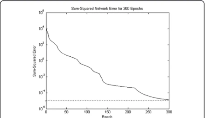
An example of training error for the neural estimator with the neural structure from Figure 6 is presented in Figure 15.
The error is decreasing after 300 training epoch using the Levenberg-Marquardt method.
The comparison transient characteristics for training and testing output data for the estimator based on ANFIS are presented in Figure 16.
The characteristics are plotted two on the same graph, to show that there is no significant difference. The acteristic of the training data is plotted with °. The char-acteristic of the FIS output is plotted with *. The difference between the training case and the testing case is very small. The plotting signs ° and * are on the same points for both characteristics. The average testing error is 2,017.10-5. The number of training epochs was 3.
If a fault appears in sensor 5, for example at the time moment of the 50th sample, an error occurs in estima-tion, like in Figure 17.
Detection of this error is equivalent to a default in sen-sor 5, from another point of view, in the place of sensen-sor 5, in the space of the distributed parameter systems, and in the heat flow around sensor 5.
Figure 12The optimised solution for meshes and nodes.
Figure 13Sensor network position in the field.
Figure 14Transient characteristics.
6.3. Comparison results
After the comparison of the results of estimation obtained using these three methods the values of the quality criterion are synthesised in the following table.
In Table 1 em is the average error,em% is the error in percentage terms related to the measured values andJis the quadratic criterion value obtained for the estimates. We may notice that the quality of estimation increases in Table 1 from top to bottom.
7. Implementation
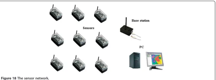
A Crossbow sensor network was used in practice (Figure 18).
The basic components of the sensor network used in practice are a base station and sensor nodes. The base station is wireless, with computing energy and com-munication resources, which is acting like an access gate between the sensor nodes and the end user. The base station is an IRIS module, a gateway MIB250, which is connected at the USB. The senor nodes have a processor/radio module IRIS, which are activating
the measuring system of small power. They are work-ing at the frequency of 2,4 GHz. The sensor circuit MTS400 includes a temperature sensor. The sensor network has also the software MoteView, for data ac-quisition, which is reading data from a database Post-rgreSQL (Figure 19).
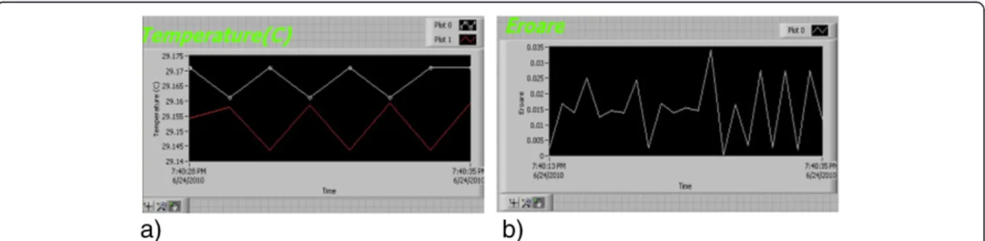
Virtual instrumentation, based on National Instru-ments technology, was used for sensor network monitor-ing. A virtual instrument was built on a personal computer, which includes: data acquisition and proces-sing, estimator, data base, results table and an Excel data base. The monitoring system is working in real time. The sampling period is 9 s. The control panel graphs for the measured and estimated temperature are presented in Figure 20a). The control panel graph for the estima-tion error is presented in Figure 20b).
The block diagram of the virtual instruments for sen-sor network monitoring is presented in Figure 21.
The block diagram is built on five levels of sub-VIs, in-cluding input–output virtual instruments and estimation sub-VIs. The coefficients of the virtual instrument are those obtained by off-line estimation. The driver assures data manipulation with a very small delay. The values obtained at long distance through the Internet are pre-sented in Figure 22.
The data are sent at long distance, on the Internet, through an ethernet connection, being visualised by a browser.
Figure 16Measured and estimated transient characteristics.
Figure 17Error at the fifth node for a fault.
Table 1 Quality results
Method em em% J
Linear 0,064 0,35 0,581
Neural 0,031 0,17 0,136
8. Conclusions
The paper has a technical contribution by implementing the scientific theory of distributed parameter systems with the linear and non-linear estimation techniques for a prac-tical application using intelligent wireless sensor networks. This approach may be seen as a new technology based on specific estimation algorithms, using the sensor network as a“distributed”sensor place in the field of the distribu-ted parameter systems, with application in the develop-ment of methods for monitoring, fault detection and diagnosis, and sensor malfunction detection.
The main contribution of this paper is a complex estima-tion structure, combining the two estimaestima-tion algorithms, with regression and auto-regression, tested separately on
other case studies, implemented using three efficient esti-mation methods: one linear and two non-linear - with neural networks and ANFIS. This complex system is used to estimate the value of the sensor at the moment t+1, based on the past values of the same sensor and also based on the current values of the adjacent sensors. The paper presents an implementation on a real sensor network of the complex estimator, using three existing fault detec-tion and diagnosis algorithms. The complex estimator uses the efficiency of the linear and non-linear implementation methods.
The identification algorithms are in accord with the distributed parameter systems. The step between the considered mathematical models and the estimation Figure 18The sensor network.
algorithms is obvious analyzing the form of the estima-tion algorithm and the general equaestima-tion of a distributed parameter system.
The aspects arising in the identification of distributed parameter systems are analysed. The structure determin-ation, variable selection and distributed computation are solved in practice.
The specific model structure imposed by the distributed parameter system dynamics is integrated into the estima-tion algorithms. The algorithms are designed based on knowledge obtained from the process seen as a distributed parameter system. The number of inputs is in accord with the process dynamics. The data acquired using sensor net-works are filtered from the associated constraints of
communication, computation and others specific to the technology of wireless sensor networks.
The sensor network has a major role in this approach, the development being done according to the modern facilities and capabilities of such an intelligent concept.
The main points of the paper may be summarised as fol-lows. Some estimation algorithms, based on regression and auto-regression, for parabolic distributed para-meters systems, are developed. They may be implemen-ted using different linear or non-linear estimation
methods–such as neural networks or ANFIS. A
moni-toring method based on a sensor network and these es-timation algorithms is presented. A case study for the heat transfer in plane is presented. The results of a Figure 20Measurements on the control panel of the virtual instrument a) The measured and estimated temperature b) The error, on the control panel of the virtual instrument.
comparison study for these three methods, based on a quadratic quality criterion, are presented. Good approx-imations were obtained for all three methods. To im-prove the quality of the estimation one of these methods could be chosen, related to the desired error and the complexity of the implementation.
A virtual instrument was developed for the sensor net-work monitoring, including an estimator, based on the esti-mator coefficients obtained in an off-line estiesti-mator design.
A long distance monitoring over the Internet is developed.
The importance of the work consists in developing new estimator methods and implementation in distrib-uted parameter systems. The main attention is given to the way in which to choose the number and the positions of the sensor nodes according to the desired accuracy in the identification process. Some examples of generated meshes and temperature estimates for different numbers of sensor are presented. A compara-tive study of how to place the sensor nodes in the field is made. A solution to know the right number of needed sensor nodes is offered. The users could know the right points in space to place the sensor nodes to obtain a good approximation by identification. The placing points are more important than the number of sensors.
A monitoring method based on a sensor network and ANFIS as estimation method for non-linear systems is presented.
The complex estimation system, based on the above estimation methods and algorithms, was developed to be implemented using virtual instrumentation.
Using this complex system the quality of estimation was improved, fact demonstrated by the good values obtained for the quadratic quality criteria.
The following applications and extensions are suggested: applications in fault detection and diagnosis of distributed parameter systems based on sensor networks and virtual instrumentation, allowing the treatment of large and com-plex systems with many variables, and also on learning and extrapolation. The monitoring method may also be applied in the case of discovery of malicious nodes in wireless sensor networks. New applications may be devel-oped in the future, considering all the capabilities of the sensor nodes to measure physical variables.
Competing interests
The authors declare that they have no competing interests.
Acknowledgement
This work was developed within the frame of PNII-IDEI-PCE-ID923-2009 CNCSIS - UEFISCSU grant.
Received: 5 December 2011 Accepted: 3 December 2012 Published: 9 January 2013
References
1. C. Volosencu, Algorithms for estimation in distributed parameter systems based on sensor networks and ANFIS. WSEAS Transactions on Systems9(3), 283–294 (2010)
2. C. Volosencu, Identification of distributed parameter systems, based on sensor networks and artificial intelligence. WSEAS Transactions on Systems7 (6), 785–801 (2008). ISSN 1109–2777
3. C. Volosencu, D.I. Curiac, Monitoring of distributed parameter systems based on a sensor network and ANFIS, in2010 IEEE World Congress on Computational Intelligence(IJCNN volume, Barcelona, Spain, 2010), pp. 2272–2279
4. C. Volosencu, Applying the technology of wireless sensor network in environment monitoring, inCutting Edge Research in New Technologies, ed. by C. Volosencu (Intech, Rijeka, 2012), pp. 97–106
5. D.I. Curiac, C. Voloşencu, A. Doboli, O. Dranga, T. Bednarz, Discovery of malicious nodes in wireless sensor networks using neural predictors. WSEAS Transactions on Computer Research2(1), 38–44 (2007). ISSN 1991–8755 6. I.F. Akyildiz, W. Su, Y. Sankarasubramaniam, E. Cayirci, Wireless sensor
networks: a survey. Computer Networks38(4) (2002)
7. B. Krishnamachari,A Wireless Sensor Networks Bibliography(University of Southern California, Technical Report, 2007)
8. R.U. Novak, U. Mira, Boundary estimation in sensor networks: theory and methods, in2nd International Workshop on Information Processing in Sensor Networks(IPSN, Palo Alto, CA, 2003)
9. G.J. Pottie, W.J. Kaiser, Wireless integrated network sensors. Communications of the ACM43(2000)
10. L. Tong, Q. Zhao, S. Adireddy,Sensor Networks with Mobile Agents, Proceedings IEEE 2003 MILCOM(, Boston, USA, 2003), pp. 688–694 11. H. Allende-Cid, A. Veloz, R. Salas, S. Chabert, H. Allende,Self Organizing
Neuro-Fuzzy System, in Progress in Pattern Recognition(Image Analysis and Applications, Springer Verlag, Heidelberg, 2008)
12. G. Battistelli, A. Benavoli, L. Chisci,State Estimation with Remote Sensors and Data Driven Communication, Estimation and Control of Networked Systems, Volume 1, Part 1, 2010(Artigianelli, Italy, 2010)
13. G. Biagetti, P. Crippa, F. Gianfelici, C. Turchetti,Sensor Network-Based Non-linear System Identification, Lecture Notes in Computer Science(Springer Berlin, Heidelberg, ), pp. 580–587
14. M. Patan, D. Ucinski, Configuring a sensor network for fault detection in distributed parameter systems. Int J Appl Math Comput Sci18(4), 513–524 (2008) 15. L. Rauchhaupt, V. Lakkundi, Wireless network integration into virtual
automation networks, inProceedings of the 17th IFAC World Congress, Volume 17, part 1(, Seoul, South Korea, 2008), pp. 13982–13987 16. M. Tubaishat, S. Mandria, Sensor networks: an overview. IEEE Potential
22(2), 20–23 (2003)
17. L. Ljung, Perspectives on system identification. Annual Reviews in Control 34(1), 1–12 (2010). Elsevier
18. P. Morreale, R. Suleski, System design and analysis of a web-based application for sensor networkdata integration and real-time presentation, in Proceedings of the 3rd IEEE Systems Conference(, Vancouver, British Columbia, Canada, 2009), pp. 201–204
19. T.P. Lambrou, C.G. Panayiotou, Collaborative area monitoring using wireless sensor networks with stationary and mobile nodes. EURASIP Journal on Advances in Signal Processing (2009). doi:10.1155/2009/750657. vol. 2009, Article ID 750657, 16 pages
20. D. Dardari, C.C. Chong, B. Damien, D.B. Jourdan, L. Mucchi, Cooperative localization in wireless ad hoc and sensor networks. EURASIP Journal on Advances in Signal Processing (2008). doi:10.1155/2008/353289. vol. 2008, Article ID 353289, 2 pages, 2008
21. V.A. Kaseva, M. Kohvakka, M. Kuorilehto, M. Hännikäinen, T.D. Hämäläinen, A wireless sensor network for rf-based indoor localization. EURASIP Journal on Advances in Signal Processing (2008). doi:10.1155/2008/731835. vol. 2008, Article ID 731835, 27 pages
22. E. Serpedin, H. Li, A. Dogandžić, H. Dai, P. Cotae, Distributed signal processing techniques for wireless sensor networks. EURASIP Journal on Advances in Signal Processing (2008). doi:10.1155/2008/540176. vol. 2008, Article ID 540176, 2 pages
23. J.C. Chen, A.G. Jaffer, Editorial. EURASIP Journal on Applied Signal Processing 2005(1), 1–3 (2005). doi:10.1155/ASP.2005.1
24. K. Yao, D. Estrin, H.Y. Hu, Editorial. EURASIP Journal on Applied Signal Processing2003(4), 319–320 (2003). doi:10.1155/S1110865703002944 25. I. Chatzigiannakis, G. Mylonas, S. Nikoletseas, The design of an environment
for monitoring and controlling remote sensor networks. International Journal of Distributed Sensor Networks5, 262–282 (2009)
26. S. Jassar, T. Behan, L. Zhao, Z. Liao, The comparison of neural network and hybrid neuro-fuzzy based inferential sensor models for space heating systems, inIEEE International Conference on Systems, Man and Cybernetics, SMC, 2009(, San Antonio, Texas, 2009), pp. 4299–4303
27. Q. Yang, A. Lim, K. Casey, R.K. Neelisetti, An enhanced CPA algorithm for real-time target tracking in wireless sensor networks. International Journal of Distributed Sensor Networks5, 619–643 (2009)
28. B. Shen, Z. Wang, Y.S. Hung, Distributed H∞-consensus filtering in sensor networks with multiple missing measurements: The finite-horizon case. Automatica46(10), 1682–1688 (2010)
29. S.H. Hsu, K.S. Chen, H.R. Lin, S.J. Chang, T.P. Tang, Effect of plasma gas flow direction on hydrophilicity of polymer by small zone cold plasma treatment
and hydrophobic plasma treatment. International Journal of Distributed Sensor Networks5, 429–436 (2009)
30. H. Zhang, J.M.F. Moura, B. Krogh, Estimation in sensor networks: a graph approach, in4th International Symposium on Information Processing in Sensor Networks(, Los Angeles, CA, 2005), pp. 203–209
31. H. Zhang, B. Krogh, J.M.F. Moura, Estimation in virtual sensor-actuator arrays using reduced-order physical models, inCDC'04 43rd IEEE Conference on Decision and Control, vol. 4 (, Bermudas, 2004), pp. 3792–3797
32. M. Farina, G. Ferrai-Trecate, R. Scattolini,Estimation and Control of Networked Systems, Vol. 1, Part 1(, Artigianelli, Italy, 2010)
33. G.C. Calafiore, F. Abrate, Distributed linear estimation over sensor networks. Int Journal of Control82(5), 1868–1882 (2009)
34. L. Shi, K.H. Johansson, M.R. Murray,Estimation Over Wireless Sensor Networks: Trade-off between Communication, Computation and Estimation Qualities, Proc. of the 17th IFAC World Congress(, Seoul, South Korea, 2008) 35. R. Saifan, O. Al-Jarrah, A novel algorithm for defending path-based denial of
service attacks in sensor networks. International Journal of Distributed Sensor Networks (2010). doi:10.1155/2010/793981. Volume 2010, Article ID 793981 36. Y.F. Zhu, H.Z. Tan, P. Wan, Y. Zhang, A blind approach to non-linear system
identification, inIET Conference on Wireless, Mobile and Sensor Networks, 2007 (CCWMSN07, Shanghai, China, 2009), pp. 209–212
37. I. Chairez, R. Fuentes, A. Poznyak, T. Poznyak, M. Escudero, L. Viana, Neural network identification of uncertain 2D partial differential equations, in6th International Conference on Electrical Engineering, Computing Science and Automatic Control, CCE, 2009(, Toluca, Mexico, 2009), pp. 1–6 38. A. Depari, A. Flammini, D. Marioli, A. Taroni, Application of an ANFIS
algorithm to sensor data processing. IEEE Trans on Instrumentation and Measurement56(1), 75–79 (2005)
39. J. Yue, J. Liu, X. Liu, W. Tan, Identification of non-linear system based on ANFIS with subtractive clustering, inThe Sixth World Congress on Intelligent Control and Automation, WCICA 2006, vol. 1 (, Dalian, China, 2006), pp. 1852–1856 40. C. De-Wang, Z. Jun-Ping, Time series prediction based on ensemble ANFIS,
inProceedings of the 2005 International Conference on Machine Learning and Cybernetics, vol. 6 (, Guangzhou, China, 2005), pp. 3552–3556
41. E. Franco, R. Olfati-Saber, T. Parisini, M.M. Polycarpou, Distributed fault diagnosis using sensor networks and consensus-based filters, in45th IEEE Conference on Decision and Control(, San Diego, CA, 2006), pp. 386–391
doi:10.1186/1687-6180-2013-4
Cite this article as:Volosencu and Curiac:Efficiency improvement in multi-sensor wireless network based estimation algorithms for distributed parameter systems with application at the heat transfer. EURASIP Journal on Advances in Signal Processing20132013:4.
Submit your manuscript to a
journal and benefi t from:
7Convenient online submission
7Rigorous peer review
7Immediate publication on acceptance
7Open access: articles freely available online
7High visibility within the fi eld
7Retaining the copyright to your article