and
Data Cloning
Thesis by
Amrit Pratap
In Partial Fulllment of the Requirements for the Degree of
Doctor of Philosophy
California Institute of Technology Pasadena, California
2008
c
° 2008
Acknowledgements
I would like to thank all the people who, through their valuable advice and support, made this work possible. First and foremost, I am grateful to thank my advisor, Dr. Yaser Abu-Mostafa for his support, assistance and guidance throughout my time at Caltech.
I would also like to thank my colleagues at the Learning Systems Group, Ling Li and Hsuan-Tien Lin, for many stimulating discussions and for their constructive input and feedback . I also would like to thank Dr. Malik Magdon-Ismail, Dr. Amir Atiya and Dr. Alexander Nicholson for their helpful suggestions.
I would like to thank the members of my thesis committee, Dr. Yaser Abu-Mostafa, Dr. Alain Martin, Dr. Pietro Perona and Dr. Jehoshua Bruck, for their time to review the thesis and all the helpful suggestions and guidance.
This thesis is in the eld of machine learning: the use of data to automatically learn a hypothesis to predict the future behavior of a system. It summarizes three of my research projects.
We rst investigate the role of margins in the phenomenal success of the Boosting Algorithms. AdaBoost (Adaptive Boosting) is an algorithm for generating an ensem-ble of hypotheses for classication. The superior out-of-sample performance of Ad-aBoost has been attributed to the fact that it can generate a classier which classies the points with a large margin of condence. This led to the development of many new algorithms focusing on optimizing the margin of condence. It was observed that directly optimizing the margins leads to a poor performance. This apparent contradiction has been the topic of a long unresolved debate in the machine-learning community. We introduce new algorithms which are expressly designed to test the margin hypothesis and provide concrete evidence which refutes the margin argument. We then propose a novel algorithm for Adaptive sampling under Monotonicity constraint. The typical learning problem takes examples of the target function as input information and produces a hypothesis that approximates the target as an output. We consider a generalization of this paradigm by taking dierent types of information as input, and producing only specic properties of the target as output. This is a very common setup which occurs in many dierent real-life settings where the samples are expensive to obtain. We show experimentally that our algorithm achieves better performance than the existing methods, such as Staircase procedure and PEST.
Acknowledgements iii
Abstract iv
1 Introduction 1
1.1 Adaptive Learning . . . 1
1.2 Data Cloning . . . 2
2 Boosting The Margins: The Need For a New Explanation 3 2.1 Notation . . . 4
2.2 AdaBoost . . . 5
2.3 AnyBoost: Boosting as Gradient Descent . . . 7
2.4 Margin Bounds . . . 9
2.5 AlphaBoost . . . 12
2.5.1 Algorithm . . . 12
2.5.2 Generalization Performance on Articial Datasets . . . 13
2.5.3 Experimental Results on Real World Datasets . . . 15
2.5.4 Discussion . . . 18
2.6 DLPBoost . . . 25
2.6.1 Algorithm . . . 25
2.6.2 Properties of DLPBoost . . . 26
2.6.3 Relationship to Margin Theory . . . 27
2.6.4 Experiments with Margins . . . 28
2.6.5.1 Articial Datasets Used . . . 30
2.6.5.2 Dependence on Training Set Size . . . 34
2.6.5.3 Dependence on the Ensemble Size . . . 37
2.6.6 Experiments on Real World Datasets . . . 40
2.7 Conclusions . . . 41
3 Adaptive Estimation Under Monotonicity Constraints 45 3.1 Introduction . . . 45
3.1.1 Applications . . . 46
3.1.2 Monotonic Estimation Setup . . . 47
3.1.3 Threshold Function . . . 47
3.1.4 Adaptive Learning Setup . . . 48
3.2 Existing Algorithms for Estimation under Monotonicity Constraint . 48 3.2.1 Parametric Estimation . . . 49
3.2.2 Non-Parametric Estimation . . . 49
3.3 Hybrid Estimation Procedure . . . 53
3.3.1 Bounded Jump Regression . . . 53
3.3.1.1 Denition . . . 53
3.3.1.2 Examples . . . 54
3.3.1.3 Solving the BJR Problem . . . 54
3.3.1.4 Special Cases . . . 55
3.3.1.5 δ as a Complexity Parameter . . . 56
3.3.2 Hybrid Estimation Algorithm . . . 57
3.3.3 Pseudo-Code and Properties . . . 58
3.3.4 Experimental Evaluation . . . 59
3.4 Adaptive Algorithms For Monotonic Estimation . . . 62
3.4.1 Maximum Likelihood Approach . . . 62
3.4.2 Staircase Procedure . . . 63
3.5 MinEnt Adaptive Framework . . . 63
4 Data Cloning for Machine Learning 77
4.1 Introduction . . . 77
4.2 Complexity of a Dataset . . . 78
4.3 Cloning a Dataset . . . 79
4.4 Learning a Cloner Function . . . 80
4.4.1 AdaBoost.Stump . . . 80
4.4.2 ρ-learning . . . 81
4.5 Data Selection . . . 83
4.5.1 ρ-values . . . 83
4.5.2 AdaBoost Margin . . . 84
4.6 Data Engine . . . 85
4.7 Experimental Evaluation . . . 85
4.7.1 Articial Datasets . . . 85
4.7.2 Complexity of Cloned Dataset . . . 86
4.7.2.1 Experimental Setup . . . 86
4.7.2.2 Results . . . 86
4.7.3 Cloning for Model Selection . . . 87
4.7.3.1 Experimental Setup . . . 87
4.7.3.2 Results . . . 87
4.7.4 Cloning for Choosing a learning algorithm . . . 97
4.7.4.1 Experimental Setup . . . 98
4.7.4.2 Results . . . 99
4.8 Conclusion . . . 99
List of Figures
2.1 Performance of AlphaBoost and AdaBoost on a Target Generated by
DEngin . . . 16
2.2 Performance of AlphaBoost and AdaBoost on a Typical Target . . . . 17
2.3 Pima Indian Diabetes DataSet . . . 19
2.4 Wisconsin Breast DataSet . . . 20
2.5 Sonar DataSet . . . 21
2.6 IonoSphere DataSet . . . 22
2.7 Votes84 Dataset . . . 23
2.8 Cleveland Heart Dataset . . . 24
2.9 Margins Distribution for WDBC Dataset with 300 Training Points . . 29
2.10 α for WDBC Dataset with 300 Training Points . . . 29
2.11 α Distribution for WDBC Dataset with 300 Training Points . . . 30
2.12 Margins Distribution for Australian Dataset with 500 Training Points . 31 2.13 α for Australian Dataset with 500 Training Points . . . 31
2.14 α Distribution for Australian Dataset with 500 Training Points . . . . 32
2.15 YinYang Dataset . . . 33
2.16 LeftSin Dataset . . . 33
2.17 Comparison of DLPBoost and AdaBoost on TwoNorm Dataset . . . . 34
2.18 Comparison of DLPBoost and AdaBoost on YinYang Dataset . . . 35
2.19 Comparison of DLPBoost and AdaBoost on RingNorm Dataset . . . . 36
2.20 Comparison of DLPBoost and AdaBoost on TwoNorm Dataset . . . . 37
2.21 Comparison of DLPBoost and AdaBoost on YinYang Dataset . . . 38
2.27 Margin Distribution on Voting Dataset . . . 43
2.28 Margin Distribution on Cancer Dataset . . . 44
3.1 δ as a Complexity Parameter Controlling the Search Space . . . 56
3.2 Comparison of Various Monotonic Estimation Methods with 1 Sample Per Bin . . . 60
3.3 Comparison of Various Monotonic Estimation Methods with m(xi) = min(i, N −i) . . . 61
3.4 MinEnt Adaptive Sampling Algorithm . . . 65
3.5 Results on Linear Target . . . 69
3.6 Results on Weibull Target . . . 70
3.7 Results on Normal Target . . . 71
3.8 Results on Student-t Distribution Target . . . 72
3.9 Results on Quadratic Target . . . 73
3.10 Results on TR Target . . . 74
3.11 Results on Exp Target . . . 75
3.12 Results on Exp2 Target . . . 76
4.1 LeftSin with 400 Examples . . . 88
4.2 LeftSin with 200 Examples . . . 89
4.3 YinYang with 400 Examples . . . 90
4.4 YinYang with 200 Examples . . . 91
4.5 TwoNorm with 400 Examples . . . 92
4.6 TwoNorm with 200 Examples . . . 93
4.7 RingNorm with 400 Examples . . . 94
4.8 RingNorm with 200 Examples . . . 95
2.1 Voting Methods Seen as Special Cases of AnyBoost . . . 9
2.2 Experimental Results on UCI Data Sets . . . 18
2.3 Experimental Results on UCI Data Sets . . . 40
3.1 Various Shapes of Target Function Used in the Comparison . . . 59
3.2 Various Shapes of Target Function Used in the Comparison . . . 66
3.3 Comparison of MinEnt with Existing Methods for Estimating50% Thresh-old . . . 67
3.4 Comparison of MinEnt with Existing Methods for Estimating 61.2% Threshold . . . 68
4.1 Performance of Cloning on LeftSin Dataset . . . 96
List of Algorithms
1 AdaBoost(S,T) [Freund and Schapire 1995] . . . 6
2 AnyBoost(C, S, T)[Mason et al. 2000b] . . . 8
3 AlphaBoost(C, S,T, A) . . . 14
4 DLPBoost . . . 26
Introduction
1.1 Adaptive Learning
The main focus of this thesis is on Adaptive Learning algorithms. In Adaptive Learn-ing, the algorithm is allowed to make decisions and adapt the learning process based on the information it already has from the existing data and settings. We consider two types of adaptive settings, the rst in which the algorithm adapts to the complexity of the dataset to add new hypothesis forming an ensemble. In the second settings, the algorithm uses the data it has to decide the optimal data-point to sample from. This is very useful in problems where the data is at premium.
the margins further has lead to worsening in performance [Li et al. 2003, Grove and Schuurmans 1998]. In this thesis, we present new variants of the AdaBoost algorithms which have been designed to test the margin explanation. Experimental results show that the margin explanation is at best incomplete.
The second setting for Adaptive learning that we consider is the more conventional approach in which the algorithm is allowed to adaptively choose a data-point. This approach has many practical implications, especially in elds where the cost of ob-taining a data-point is very high. The typical learning problem takes examples of the target function as input information and produces a hypothesis that approximates the target as an output. We consider a generalization of this paradigm by taking dierent types of information as input, and producing only specic properties of the target as output. We present new algorithms for estimating under monotonicity constraint and adaptively selecting the next data-point.
1.2 Data Cloning
Boosting The Margins: The Need For
a New Explanation
In any learning scenario, the main goal is to nd a hypothesis that performs well on the unseen examples. In recent years, there has been a growing interest in voting algorithms, which combine the output of many hypotheses to produce a nal output. These algorithms take a given base learning algorithm and apply it repeatedly to re-weighted versions of the original dataset, thus producing an ensemble of hypotheses which are then combined via a weighted voting scheme to form a nal aggregate hypothesis.
AdaBoost [Freund and Schapire 1995] is the most popular and successful of the boosting algorithms. It has been successfully applied to many real-world problems with huge success [Guo and Zhang 2001, Schapire and Singer 2000, Schwenk and Ben-gio 1997, Schwenk 1999]. One interesting experimental observation about AdaBoost is that it continues to improve the out-of-sample error even when the training error has converged to zero [Breiman 1996, Schapire et al. 1997]. This is a very surpris-ing property as it goes against the principle of Occam's razor which favors simpler explanations.
[2000b] showed that AdaBoost does gradient descent optimization on the soft-min of the margin in a functional space. There are theoretical bounds on the out-of-sample performance of an ensemble classier which depends on the fraction of training points with small margin. It has however been observed that directly optimizing the min-imum margin leads to poor performance [Grove and Schuurmans 1998]. There has been a long debate in the machine-learning community about the validity of the mar-gin explanation [Breiman 1994; 1996; 1998; 1999, Schapire et al. 1997, Reyzin and Schapire 2006]. We propose variants of the boosting algorithm and prove empirically that the margin explanation is at best incomplete and motivates the need for a new explanation which would lead to the design of better algorithms for machine learning. We will rst introduce the notation and then describe the AdaBoost algorithm and its generalization, AnyBoost. We discuss the bounds provided by the margin theory. We introduce two variants of AdaBoost AlphaBoost and DLPBoost and discuss the results, which empirically refute the margin explanation and motivate the need for a new explanation.
2.1 Notation
We assume that the examples (x, y) are randomly generated from some unknown
probability distributionD onX ×Y, whereX is the input space andY is the output
space. We will only be dealing with binary classiers, so in general we will have
Y = {−1,1}. Boosting algorithms produce a voted combination of classiers of the
formsgn(F(x)) where
F(x) =
T
X
t=1
αtft(x)
where ft : X → {−1,1} are base classiers from some xed hypothesis class F,
and αt ∈ R+with PTt=1αt = 1 are the weights of the classiers. The class of all
learning is to construct a hypothesis in our case a voted combination of classier so that it minimizes the out-of-sample error which is dened asπ =PD[sgn(F(x))6=
y], i.e., the probability that F wrongly classies a random point drawn from the
distributionD. The in-sample distribution over the training points would be denoted
byS , with the in-sample error dened as ν =PS[sgn(F(x))6=y].
2.2 AdaBoost
AdaBoost is one of the most popular boosting algorithms. It takes a base learning algorithm and repeatedly applies it to re-weighted versions of the original training sample, producing a linear combination of hypothesis from the base learner. At each iteration, AdaBoost emphasizes the misclassied examples from the previous itera-tion, thereby forcing the weak learner to focus on the dicult examples. Algorithm 1 gives the pseudo-code of AdaBoost.
The eectiveness of AdaBoost has been attributed to the fact that it tends to produce classiers with large margins on the training points. Theorem 1 bounds the generalization error of a voted classier in terms of the fraction of points with a small margin.
Theorem 1 [Schapire et al. 1997]
Let S be a sample of N examples chosen independently at random according to
D. Assume that the base hypothesis space F has VC-dimension d, and let δ > 0.
Then with probability at least 1−δ over the random choice of the training set S,every
Algorithm 1 AdaBoost(S,T) [Freund and Schapire 1995]
• Input: S = (x1, y1), ...,(xN, yN)
• Input: T the number of iterations
• Initialize wi = N1 fori= 1, .., N
• Fort = 1 toT do
Train the weak learner on the weighted dataset (S, w) and obtain ht: : X→ {−1,1}
Calculate the weighted training error²t of ht:
²t= N
X
i=1
wiI[ht(xi)6=yi]
Calculate the weightαt as:
αt=
1 2log
1−²t
²t
Update weights
wnewi =wiexp{−αtynht(xn)}/Zt
whereZt is a normalization constant
if ²t= 0 or ²t≥ 12 then break and set T =t−1
• OutputFT(x) = PtT=0αtht(x)
PD[sgn(F(x))6=y] ≤ PS[yF(x)≤γ] +O
Ãr
γ−2dlog(N/d) + log(1/δ) N
!
perfor-Mason et al. [2000b] presents a generalized view of boosting algorithms as a gradient descent procedure in the functional space. Their algorithm, AnyBoost, iteratively minimizes the cost function by gradient descent in the functional space.
The base hypotheses and their linear combinations can be viewed as elements of an inner product space (C,D), where C is a linear space of functions that contain lin(F), a generalization of conv(F). The algorithm AnyBoost starts with the zero
function F and iteratively nds a functionf ∈ F to add to F so as to minimize the
cost C(F +²f) for some small ². The new added function f is chosen such that the
cost function is maximally decreased. The desired direction is the negative of the functional derivative of C atF, −∇C(F), where
∇C(F)(x) := ∂C(F +δ1x)
∂δ |δ=0
where 1x is the indicator function of x. In general it is not possible to choose the
new function as the negative of the gradient since we are restricted to picking fromF,
so instead AnyBoost searches forf which maximizes the inner producthf,−∇C(F)i
Most of the boosting algorithms use a cost function of the margin of points:
C(F) = 1
N
N
X
i=1
c(yiF(xi))
where c : R → R+is a monotonically non-decreasing function. In this case, the
inner product can be dened as
hf, gi= 1 N
N
X
i=1
f(xi)g(xi) (2.1)
Algorithm 2 AnyBoost(C, S, T) [Mason et al. 2000b]
Requires:
• An inner product space (X,h,i)containing functions mapping X toY
• A class of base classier F
• A dierentiable cost functional C :lin(F)→ ℜ
• A weak learner L(F) that accepts F ∈lin(F) and returns f ∈ F with a large
value of − h∇C(F), fi
• Input: S = (x1, y1), ...,(xN, yN)
• Input: T is the number of iterations
Let F0(x) := 0
fort = 0 toT do
∗ Let ft+1 :=L(Ft)
∗ if − hf,−∇C(F)i ≤0
· return Ft
∗ Choose αt+1
∗ Let Ft+1 =Ft+αt+1ft+1
AdaBoost can be seen as a special case of AnyBoost with the cost function
c(yF(x)) = e−yF(x)and the inner product hF(x), G(x)i = 1
N
PN
i=1F(xi)G(xi). Many
of the most successful voting methods are special cases of AnyBoost with the appro-priate cost function and step size.
Table 2.1: Voting Methods Seen as Special Cases of AnyBoost Algorithm Cost Function Step Size
AdaBoost e−yF(x) Line Search
ARC-X4 (1−yF(x))5 1/t
LogitBoost ln(1 +e−yF(x)) Newton-Rapson
2.4 Margin Bounds
The most popular explanation for the performance of AdaBoost is that it tends to produce classiers which have large margins on the training points. This has lead to a great deal of development in algorithms which can optimize the margins [Boser et al. 1992, Demiriz et al. 2002, Grove and Schuurmans 1998, Li et al. 2003, Mason et al. 2000a]. Schapire et al. [1997] introduced the margin explanation and provided a bound for the generalization performance of the AdaBoost solution. Theorem 1 bounds the generalization performance by the fraction of training points which have a small margin and a complexity term. This was improved by Koltchinskii and Panchenko [2002]
PD[yF(x)≤0]≤ inf
δ∈(0,1] PS[yF(x)≤δ] +
C δ
V(H)
n +
log log2(2δ−1) n
+
r
1 2nlog
2 ²
Experimentally it has been observed that this bound is very loose. It has been shown that as long as the VC-Dimension of the base classier used in the boosting process is small, the margin bound can be improved. Koltchinskii et al. [2000a] introduced a new class of bounds called the γ-bounds. If the base classiers belong
to a model with a small random entropy, then the generalization performance can be further bound based on the growth rate of the entropy. Given a metric space
(F, d), the ²−entropy of F, denoted by Hd(F;²) is dened as logNd(F;²), where
Nd(F;²) is the minimum number of ²−balls covering F. The γ−margin δ(γ;f) and
the corresponding empirical γ-margin δˆ(γ;f) are dened as
δ(γ;f) = supδ ∈(0,1) :δγP{yf(x)≤δ} ≤n−1+γ/2
ˆ
δ(γ;f) = supδ∈(0,1) :δγPS{yf(x)≤δ} ≤n−1+γ/2
Theorem 3 Suppose that for some α∈(0,2) and some constant D
HdPn,2(conv(F;u)≤Du
−α, u >0a.s.
then for any γ ≥ 2+2αα, for some constants A, B >0 and for large enough n
P h∀f ∈ F :A−1δˆn(γ;f)≤δn(γ;f)≤Aδˆn(γ;f)
i
≥1−B(log2log2n) exp−nγ/2/2
The random entropy of the convex hull of a model can be bounded in terms of its VC-dimension.
HdPn,2(conv(H;u)≤ sup
Q∈P(S)
HdQ,2(conv(H;u)≤Du
−2V−1
The bound is the weakest for γ = 1, and at this value it reduces to the bound
in Theorem 2. Smaller values of γ give a better generalization bound. So, if the
base classier has a very low VC-dimension, then this gives a much tighter bound on the generalization performance. It has been observed empirically, that the bound holds for smaller values of γ than what has been proved. The conjecture is that the
classiers produced by boosting belong to a subset of the convex hull, which has a smaller random entropy than the whole convex hull.
Koltchinskii et al. [2000a] provided new bounds for the generalization performance which uses the dimensional complexity of the generated classier as a measure of complexity. The dimensional complexity measures how fast the weights given to the hypothesis decrease in the ensemble. For a function F ∈Conv(F), the approximate ∆-dimension is dened as the integer d ≥ 0 such that there exists N ≥ 1, functions
fj ∈ F,j = 1, .., N and numbersλj ∈ ℜ, satisfyingF =PjN=1λjfj,PNj=1|λj|= 1 and
PN
j=d+1|λj| ≤∆. The ∆-dimension of F is denoted as d(F,∆).
Theorem 4 If H ⊂Conv(F) is a class of functions such that for some β >0
sup
F∈H
d(F, δ) =O(∆−β)
then with high probability, for any h∈ H, the generalization error can be bounded
by
1
n1−γβ/2(γ+β)δˆ(h)γβ/(γ+β)
The proof and discussion about these bounds can be found in Koltchinskii et al. [2000a;b] and Koltchinskii and Panchenko [2002]
2.5 AlphaBoost
In this section, we introduce an algorithm which produces an ensemble with much lower value for the cost function than AdaBoost. AlphaBoost improves on AnyBoost by minimizing the cost function more aggressively. It can achieve signicantly lower values of cost function much faster than AnyBoost. AnyBoost is an iterative algorithm which is restricted to adding new hypothesis and the corresponding weight to the ensemble. It can not go back and change the weights it had assigned to a hypothesis.
2.5.1 Algorithm
AlphaBoost starts out by calling AnyBoost to obtain a linear combination of hypothe-ses from the base learner. It then optimizes the weights given to each of the classier in the combination to further reduce the cost function. This is done by doing a con-jugate gradient descent [Fletcher and Reeves 1964] in the weight space. Algorithm 3 gives the pseudo-code of AlphaBoost. We used conjugate gradient instead of normal gradient descent because it uses the second-order information of the cost function and so the cost is reduced faster.
The rst step is to visualize the cost function as a function of the weight of the hypotheses, rather than of the aggregate hypothesis. So once we've xed the base learners which will vote to form the aggregate hypothesis, we have a cost function
C(α) which depends on the weight each hypothesis gets in the aggregate. We can
then do a conjugate gradient descent in the weight space to minimize the cost function and thus nd the optimal weights.
Suppose AnyBoost returns FT(x)=PiT=1αihi(x)as the nal hypothesis. Then we
∂C(α) ∂αt
=X
i=1
yiht(xi)c′(yiFT(xi)) (2.4)
So the descent direction at staget is computed asdt=−∇C(αt). Instead of using
this direction directly, we choose the search direction as
dt=−∇C(αt) +βtdt−1 (2.5)
where βt ∈ ℜ and dt−1 is the last search direction. The value of βt controls how
much of the previous direction aects the current direction. It is computed using the Polak-Ribiere formula
βt= h
dt, dt−dt−1i
hdt−1, dt−1i (2.6)
Algorithm 3 uses a xed step size to perform conjugate descent. We can also do a line search to nd an optimal step size at each iteration.
2.5.2 Generalization Performance on Articial Datasets
For analyzing the out-of-sample performance of AlphaBoost, we used AdaBoost's exponential cost function. Once we x a cost function, AnyBoost, which reduces to AdaBoost in this case, and AlphaBoost are essentially two algorithms which try to optimize the same cost function.
pa-Algorithm 3 AlphaBoost(C, S,T, A)
Requires:
• An inner product space (X,h,i)containing functions mapping X toY
• A class of base classier F
• Input: S = (x1, y1), ...,(xN, yN)
• Input : T the number of iterations of AnyBoost andAis the number of conjugate
gradient steps
• Input: C is a dierentiable cost functional C :lin(F)→ ℜ
Let FT(x)=α.H(x) be the output of AnyBoost(C,S,T)
d0 = 0 and α0 =α
For t = 1to A
∗ dt =−∇C(αt)
∗ βt = hhddtt,dt−dt−1i
−1,dt−1i
∗ dαt=−dt+βtdαt−1
∗ αt=αt−1+ηdαt−1
rameters for that model, and produces random examples according to the generated model. A complexity factor can be specied which controls the complexity of the generated model. The engine can be prompted repeatedly to generate independent data sets from the same model to achieve small error bars in testing and comparing learning algorithms.
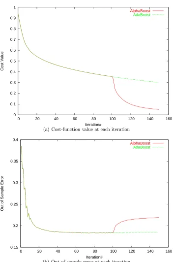
The two algorithms were compared using function of varying complexity and from dierent models. For each target, 100 independent training sets of size 500 were
generated. The algorithms were tested on an independently generated test set of size
5000. AlphaBoost was composed of 100 steps of AdaBoost, followed by 50 steps of
conjugate gradient with line search, and it was compared with AdaBoost running for 150 iterations. In all the runs, AlphaBoost obtained signicantly lower values of
cost function. However, the out-of-sample performance of AdaBoost was signicantly better.
algo-The cost function at the end of AlphaBoost is signicantly lower than the cost function at the end of AdaBoost. However, the out-of-sample error achieved by AdaBoost is signicantly lower.
2.5.3 Experimental Results on Real World Datasets
We tested AlphaBoost on six datasets from the UCI machine learning repository[Blake and Merz 1998]. The datasets were the Pima Indians Diabetes Database; sonar database; heart disease diagnosis database from V.A. Medical Center, Long Beach; and Cleveland Clinic Foundation collected by Robert Detrano, M.D., Ph.D. Johns Hopkins University Ionosphere database, 1984; United States Congressional Voting Records Database; and breast cancer databases from the University of Wisconsin Hospitals [Mangasarian and Wolberg 1990]. Decision stumps were used as the base learner in all the experiments. For the experiments, the dataset was randomly divided into two sets of size 80% and 20% and they were used for training and testing the
algorithms. AlphaBoost was composed of100 steps of AdaBoost, followed by50steps
of conjugate gradient with line search as in the previous section and it was compared with AdaBoost running for150 iterations. All the results were averaged over50runs.
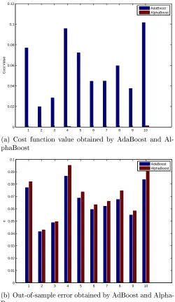
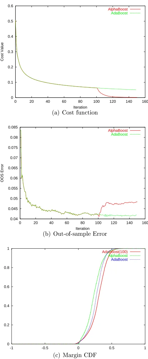
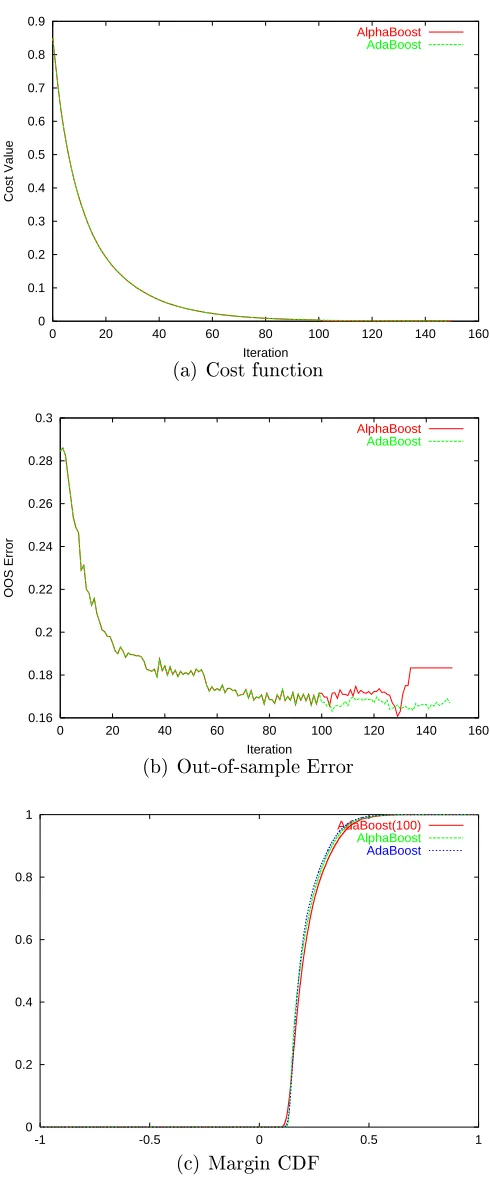
Table 2.2 shows the nal values obtained by the two algorithms. As expected, AlphaBoost was able to achieve signicantly lower value of the cost function. Though AdaBoost achieved better out-of-sample error than AlphaBoost, the error bars are too high in these limited datasets to make any statistically signicant conclusions. Figures 2.32.8 show the cost function value and out-of-sample error as a function of the number of iterations. For the rst 100 iterations, AdaBoost and AlphaBoost
1 2 3 4 5 6 7 8 9 10 0
0.02 0.04 0.06 0.08 0.1 0.12
Cost Value
AdaBoost AlphaBoost
(a) Cost function value obtained by AdaBoost and Al-phaBoost
1 2 3 4 5 6 7 8 9 10
0 0.01 0.02 0.03 0.04 0.05 0.06 0.07 0.08 0.09 0.1
π
AdaBoost AlphaBoost
(b) Out-of-sample error obtained by AdBoost and Alpha-Boost
0 0.1 0.2 0.3 0.4 0.5 0.6 0.7
0 20 40 60 80 100 120 140 160
Cost Value
Iteration#
(a) Cost-function value at each iteration
0.15 0.2 0.25 0.3 0.35 0.4
0 20 40 60 80 100 120 140 160
Out of Sample Error
Iteration#
AlphaBoost
AdaBoost
(b) Out-of-sample error at each iteration
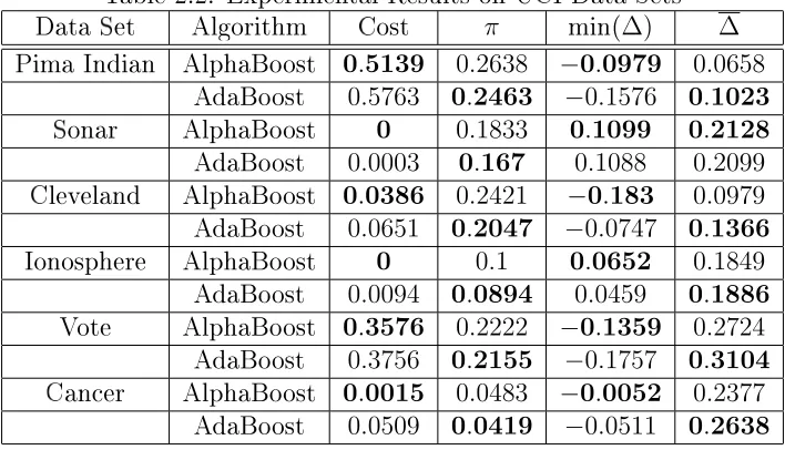
Table 2.2: Experimental Results on UCI Data Sets
Data Set Algorithm Cost π min(∆) ∆
Pima Indian AlphaBoost 0.5139 0.2638 −0.0979 0.0658
AdaBoost 0.5763 0.2463 −0.1576 0.1023
Sonar AlphaBoost 0 0.1833 0.1099 0.2128
AdaBoost 0.0003 0.167 0.1088 0.2099
Cleveland AlphaBoost 0.0386 0.2421 −0.183 0.0979
AdaBoost 0.0651 0.2047 −0.0747 0.1366
Ionosphere AlphaBoost 0 0.1 0.0652 0.1849
AdaBoost 0.0094 0.0894 0.0459 0.1886
Vote AlphaBoost 0.3576 0.2222 −0.1359 0.2724
AdaBoost 0.3756 0.2155 −0.1757 0.3104
Cancer AlphaBoost 0.0015 0.0483 −0.0052 0.2377
AdaBoost 0.0509 0.0419 −0.0511 0.2638
gradient descent. The out-of-sample error increases during this stage. Also shown are the distribution of the margins at the end of 100 iterations of AdaBoost, and at the
end of100iterations of AdaBoost and50iterations of conjugate gradient descent. The
distribution of the margins at the end of 100 iterations of AdaBoost is the starting
point for both the algorithms, and from that point forward, they do dierent things for the next50iterations. AlphaBoost tends to maximize the minimum margin better
than AdaBoost at the expense of lowering the maximum margin.
2.5.4 Discussion
0.5 0.55 0.6 0.65 0.7
0 20 40 60 80 100 120 140 160
Cost Value
Iteration
(a) Cost function
0.24 0.245 0.25 0.255 0.26 0.265 0.27 0.275 0.28
0 20 40 60 80 100 120 140 160
OOS Error
Iteration
AlphaBoost AdaBoost
(b) Out-of-sample Error
0 0.2 0.4 0.6 0.8 1
-1 -0.5 0 0.5 1
AdaBoost(100) AlphaBoost AdaBoost
(c) Margin CDF
0 0.1 0.2 0.3 0.4 0.5 0.6
0 20 40 60 80 100 120 140 160
Cost Value
Iteration
AlphaBoost AdaBoost
(a) Cost function
0.04 0.045 0.05 0.055 0.06 0.065 0.07 0.075 0.08 0.085
0 20 40 60 80 100 120 140 160
OOS Error
Iteration
AlphaBoost AdaBoost
(b) Out-of-sample Error
0 0.2 0.4 0.6 0.8 1
-1 -0.5 0 0.5 1
AdaBoost(100) AlphaBoost AdaBoost
(c) Margin CDF
0 0.1 0.2 0.3 0.4
0 20 40 60 80 100 120 140 160
Cost Value
Iteration
(a) Cost function
0.16 0.18 0.2 0.22 0.24 0.26 0.28 0.3
0 20 40 60 80 100 120 140 160
OOS Error
Iteration
AlphaBoost AdaBoost
(b) Out-of-sample Error
0 0.2 0.4 0.6 0.8 1
-1 -0.5 0 0.5 1
AdaBoost(100) AlphaBoost AdaBoost
(c) Margin CDF
0 0.1 0.2 0.3 0.4 0.5 0.6 0.7 0.8
0 20 40 60 80 100 120 140 160
Cost Value
Iteration
AlphaBoost AdaBoost
(a) Cost function
0.08 0.09 0.1 0.11 0.12 0.13 0.14 0.15 0.16 0.17 0.18
0 20 40 60 80 100 120 140 160
OOS Error
Iteration
AlphaBoost AdaBoost
(b) Out-of-sample Error
0 0.2 0.4 0.6 0.8 1
-1 -0.5 0 0.5 1
AdaBoost(100) AlphaBoost AdaBoost
(c) Margin CDF
0.35 0.4 0.45 0.5 0.55
0 20 40 60 80 100 120 140 160
Cost Value
Iteration
(a) Cost function
0.19 0.2 0.21 0.22 0.23 0.24 0.25 0.26 0.27 0.28
0 20 40 60 80 100 120 140 160
OOS Error
Iteration
AlphaBoost AdaBoost
(b) Out-of-sample Error
0 0.2 0.4 0.6 0.8 1
-1 -0.5 0 0.5 1
AdaBoost(100) AlphaBoost AdaBoost
(c) Margin CDF
0 0.1 0.2 0.3 0.4 0.5 0.6 0.7 0.8 0.9
0 20 40 60 80 100 120 140 160
Cost Value
Iteration
AlphaBoost AdaBoost
(a) Cost function
0.19 0.2 0.21 0.22 0.23 0.24 0.25 0.26 0.27
0 20 40 60 80 100 120 140 160
OOS Error
Iteration
AlphaBoost AdaBoost
(b) Out-of-sample Error
0 0.2 0.4 0.6 0.8 1
-1 -0.5 0 0.5 1
AdaBoost(100) AlphaBoost AdaBoost
(c) Margin CDF
DLPBoost is an extension of AdaBoost which optimizes the margin distribution pro-duced by AdaBoost. It has been expressly designed to test the margin explanation for the performance of AdaBoost. We have seen in the case of AlphaBoost that decreasing the cost function leads to larger minimum margin, but at the expense of decreasing the margin of some of the points. In most of the extensions and variants of AdaBoost, the margin distribution produced does not dominate the margin distribu-tion of AdaBoost. We say that a distribudistribu-tionP1 dominates another distributionP2 if P1(t)≤P2(t),∀t. As a result, there are some cost functions of the margin that would
be worsened by the variant. The only algorithm which could produce a better margin distribution was Arc-gv [Breiman 1998]. This algorithm was, however, criticized for producing complex hypotheses and hence the increase in error was attributed to the additional complexity used [Reyzin and Schapire 2006]. This is an important consid-eration in the design of DLPBoost. We want to make sure that the dierence in the solutions of AdaBoost and DLPBoost can only be accounted for by the dierence in the margins. It is therefore crucial to keep all other factors constant.
In DLPBoost, we provide an algorithm which consistently improves the entire distribution of the margins. This condition ensures that DLPBoost has a better margin cost than AdaBoost for any possible denition of margin cost. Thus, all the margin bounds for AdaBoost would hold for DLPBoost, and as the complexity terms are not changed, the bounds become tighter. This would lead to better performance if the margin explanation is true.
2.6.1 Algorithm
Algorithm 4 DLPBoost Given (x1, y1), ...,(xN, yN)
Run AdaBoost/AnyBoost for T iterations to get(h1, ..., hT) and (α∗1, ..., αT∗)
Denem(α, i) =PT
t=1yiαtht(xi)
Solve the linear programming problem
maxαPNi=1m(α, i)
Subject to constraints
m(α, i)≥m(α∗, i)
P
αt= 1,αt ≥0
improving the margin distribution is very hard, optimization-wise, as it also involves a combinatorial component. So, instead we set up a restricted problem in which we require that the margin on none of the points is decreased. Any solution of the latter problem would be a feasible solution for the original problem, though it might not be optimal. Our goal here is to produce better margin distribution, and the restricted setup ensures that any solution we produce would have margin distributions at least as good as those of the AdaBoost solution.
Algorithm 4 illustrates DLPBoost. The base classiers produced by DLPBoost are the exact same as the one produced by AdaBoost, and, by design, the margin of each training example is not reduced. Thus, by denition, DLPBoost does not cheat on the complexity and produces a solution which dominates (or at least equals) the margin distribution produced by AdaBoost.
2.6.2 Properties of DLPBoost
DLPBoost uses linear programming to nd new weights for the hypotheses which would maximize the average margin, while ensuring that all the training examples have a margin at least as large as that of the AdaBoost solution. The weights gen-erated by AdaBoost, α∗, are a feasible solution to the optimization problem in
the DLPBoost solution can be useful as it tends to have a smaller ensemble size. One of the interesting aspects of the DLPBoost setup is that the function being optimized is ad hoc. The important thing is to nd a non-trivial feasible solution to the constraints. The trivial solution in this case would be the AdaBoost solution in which all the inequalities are exactly satised. We have used the average margin as the goal, but we can use any general linear combination of the margins as the goal and still have a working setup. The most general setup would be a Multi-objective optimization setup, in which we can maximize the margin on each point. There are popular algorithms [Deb et al. 2002] to solve this kind of problem but we do not use those, as the added advantage of a sparse solution generated by linear programming is very appealing in our case. In addition, any non-trivial feasible solution would be an added improvement on the margin distribution and serve the purpose of our analysis.
2.6.3 Relationship to Margin Theory
All the bounds discussed in section 2.4 hold for DLPBoost. For DLPBoost, by de-nition
∀δPS[yFD(x)≤δ]≤PS[yFA(x)≤δ]
(where FD is the DLPBoost solution and FA is the AdaBoost solution). Hence we
have that the bound on the generalization error of DLPBoost is smaller than the bound on the generalization error of AdaBoost.
which can also be used to generate ensembles with better margin distribution, has been criticized for using additional hypothesis complexity [Reyzin and Schapire 2006]. It also uses hypotheses which are dierent from those used by AdaBoost, and so it is plausible that the solution generated is more complicated, thus any negative results there might not contradict the margin explanation. In DLPBoost, we have isolated the margin explanation and any dierence in performance can only be accounted for by the dierence in the margin distributions. This would give us a fair evaluation of the margin explanation.
2.6.4 Experiments with Margins
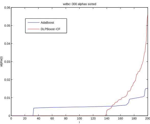
We study the behavior of the margins and the solution produced by DLPBoost. Figures 2.9, 2.10 and 2.11 show the margins and the weights on the hypotheses ob-tained by AdaBoost and DLPBoost on the WDBC dataset. In this setup, we weight the margins of the points in the linear programming setup by their cost function. This weighing promotes the points with smaller margin. The out-of-sample errors for AdaBoost was 2.74% and for DLPBoost was 3.75%. The margin distribution for
DLPBoost is clearly much better than that of AdaBoost, and from the nal weights obtained, we can see that the hypotheses removed from the AdaBoost solution by DLPBoost had signicant weights assigned to them. Figure 2.10 shows the weights assigned by the two algorithms to the weak hypotheses which are indexed by the iteration number. It can be seen that DLPBoost emphasizes some hypotheses which were generated late in AdaBoost training and it also killed some of the hypotheses which were generated early. AdaBoost is a greedy iterative algorithm. This kind of behavior is expected, as AdaBoost has no way of going back and correcting the weights of hypotheses already generated. Note that the one-norm of both the solu-tions is normalized to one, and so the DLPBoost solution having a smaller number of hypotheses (64, compared to the 168 of AdaBoost) has overall larger weights and
this result is for a single run.
0 0.1 0.2 0.3 0.4 0.5 0.6 0.7 0.8 0.9 1 0
0.1 0.2 0.3 0.4 0.5 0.6 0.7
margin
Figure 2.9: Margins Distribution for WDBC Dataset with 300 Training Points
0 20 40 60 80 100 120 140 160 180 200
0 0.01 0.02 0.03 0.04 0.05 0.06
iteration #
alpha(i)
wdbc−300 alphas
AdaBoost DLPBoost−CF
0 20 40 60 80 100 120 140 160 180 200 0
0.01 0.02 0.03 0.04 0.05 0.06
i
alpha(i)
wdbc−300 alphas sorted
AdaBoost DLPBoost−CF
Figure 2.11: α Distribution for WDBC Dataset with 300 Training Points
dataset. Here the errors for both the algorithms were 18.8% while the number of
hypotheses was reduced from423to201. In this case, there is very small improvement
in the margin distribution and the out-of-sample error did not change. The hypotheses killed by the DLPBoost step had signicant weights.
This points to an inverse relationship between the margins and the out-of-sample performance. In the next two sections, we will investigate this relationship in detail and give statistically signicant results.
2.6.5 Experiments with Articial Datasets
We test the performance of DLPBoost and compare it with that of AdaBoost on a few articial datasets.
2.6.5.1 Articial Datasets Used
We used the following articial learning problems for evaluation the performance of the cloning process.
0 0.05 0.1 0.15 0.2 0.25 0.3 0.35 0.4 0
0.1 0.2 0.3 0.4 0.5 0.6 0.7
margin
Figure 2.12: Margins Distribution for Australian Dataset with 500 Training Points
0 50 100 150 200 250 300 350 400 450 500 0
0.01 0.02 0.03 0.04 0.05 0.06 0.07
aus−500 alphas
iteration #
alpha(i)
0 50 100 150 200 250 300 350 400 450 500 0 0.01 0.02 0.03 0.04 0.05 0.06 0.07 aus−500 alphas i alpha(i)
Figure 2.14: α Distribution for Australian Dataset with 500 Training Points
rst class includes all points (x1, x2)which satises
(d+ ≤r)∨
¡
r < d− ≤ R2
¢
∨¡
x2 >0∧d+ > R2
¢
,
where the radius of the plate is R = 1 and the radius of the two small circles is r= 0.18, d+ =
q
(x1− R2)2+x22 and d− =
q
(x1+ R2)2+x22.
LeftSin ([Merler et al. 2004]) partitions[−10,10]×[−5,5]into two class regions with
the boundary
x2 =
2 sin 3x1, if x1 <0;
0, if x1 ≥0.
TwoNorm ([Breiman 1996]) is a20-dimensional,2-class classication dataset. Each
class is drawn from a multivariate normal distribution with unit variance. Class
1has mean(a, a, ..a)while Class2has mean (−a,−a, ..−a), wherea= 2/√20.
Figure 2.15: YinYang Dataset
0 200 400 600 800 1000 1200 1400 1600 1800 2000 2200 −2 0 2 4 6 8 10 12 14 N πdlp − πada
(a) Change inπ
0 200 400 600 800 1000 1200 1400 1600 1800 2000 2200 0 0.005 0.01 0.015 0.02 0.025 0.03 0.035 0.04 N
(b) Change in Average Margin
0 200 400 600 800 1000 1200 1400 1600 1800 2000 2200 0 0.05 0.1 0.15 0.2 0.25 N
(c) Maximum Change in Margin
200 400 600 800 1000 1200 1400 1600 1800 2000 2200 0 50 100 150 200 250 300 350 400 450 N AdaBoost DLPBoost
(d) Size of Ensemble
Figure 2.17: Comparison of DLPBoost and AdaBoost on TwoNorm Dataset
2.6.5.2 Dependence on Training Set Size
In the rst test, we evaluate the dierence in performance between AdaBoost and DLPBoost. We evaluate the dierence in the out-of-sample error, the average change in the margin on the training points, and the maximum change in the margin. We also compare the number of hypothesis which have non-zero weight in the ensembles of AdaBoost and DLPBoost. Each of the simulations used an independent set of training and test points and was run for500 iterations of AdaBoost with the training
set size varying from 200 to 2000. All the results are averaged over 100 independent
0 500 1000 1500 2000 2500 3000 −1
0 1
N
(a) Change inπ
0 500 1000 1500 2000 2500 3000
0 0.2 0.4
N
(b) Change in Average Margin
0 500 1000 1500 2000 2500 3000
0 0.5 1 1.5 2 2.5 3 3.5 4 4.5
5x 10
−3
N
(c) Maximum Change in Margin
0 500 1000 1500 2000 2500 3000
0 1 2 3 4 5 6 7 8 9 10 N AdaBoost DLPBoost
(d) Size of Ensemble
Figure 2.18: Comparison of DLPBoost and AdaBoost on YinYang Dataset
Figure 2.17 shows the results for the TwoNorm dataset, which is 20-dimensional.
We observe that the out-of-sample performance of DLPBoost is consistently worse than that of AdaBoost. The dierence goes down to zero as the training set size increases. The increase in the average margins and the maximum change in the margin are indications of the ineciency of AdaBoost in optimizing the margins. We can also see the number of hypotheses used by the DLPBoost increase as we increase the training set size.
We observe similar behavior on the Yin-Yang dataset (Figure 2.18) which is 2
0 200 400 600 800 1000 1200 1400 1600 1800 2000 2200 0 0.002 0.004 0.006 0.008 0.01 0.012 N πdlp − πada
(a) Change in π
0 200 400 600 800 1000 1200 1400 1600 1800 2000 2200 0 0.01 0.02 0.03 0.04 0.05 0.06 N
(b) Change in Average Margin
0 200 400 600 800 1000 1200 1400 1600 1800 2000 2200 0 0.05 0.1 0.15 0.2 0.25 N
(c) Maximum Change in Margin
200 400 600 800 1000 1200 1400 1600 1800 2000 2200 0 50 100 150 200 250 300 350 400 450 N AdaBoost DLPBoost
(d) Size of Ensemble
Figure 2.19: Comparison of DLPBoost and AdaBoost on RingNorm Dataset
not signicantly dierent from0in most of the cases. Another observation here is that
even for3000points in the training set, the DLPBoost solution does not use all the500
hypotheses. In the TwoNorm case, with large training sets, the DLPBoost solution used all the 500 hypotheses in its solution. Hence the ineciency in AdaBoost is a
function of the complexity of the dataset and the number of examples in the training points. AdaBoost ended up using 500hypotheses to explain the Yin-Yang dataset of 1000 examples or more which is a clear indication of over tting. DLPBoost, on the
other hand, adjusts its complexity based on the complexity of the dataset.
0 200 400 600 800 1000 1200 1400 1600 1800 2000 2200 0
0.001 0.002 0.003 0.004
T
(a) Change in π
0 200 400 600 800 1000 1200 1400 1600 1800 2000 2200 0
0.01 0.02
T
(b) Change in Average Margin
0 200 400 600 800 1000 1200 1400 1600 1800 2000 2200 0
0.05 0.1 0.15 0.2 0.25
T
(c) Maximum Change in Margin
200 400 600 800 1000 1200 1400 1600 1800 2000 2200 0
500 1000 1500
T AdaBoost
DLPBoost
(d) Size of Ensemble
Figure 2.20: Comparison of DLPBoost and AdaBoost on TwoNorm Dataset
reected in the results in Figure 2.19.
2.6.5.3 Dependence on the Ensemble Size
We ran the same experiments by xing the ensemble size to 500 and varying the
number of iterations given to AdaBoost. Figures (2.202.22) give the results of these experiments.
0 200 400 600 800 1000 1200 1400 1600 1800 2000 2200 −2 0 2 4 6 8 10 12 14 16x 10
−4
T πdlp
−
πada
(a) Change inπ
0 200 400 600 800 1000 1200 1400 1600 1800 2000 2200 0 0.002 0.004 0.006 0.008 0.01 0.012 0.014 T
(b) Change in Average Margin
0 200 400 600 800 1000 1200 1400 1600 1800 2000 2200 0.03 0.04 0.05 0.06 0.07 0.08 0.09 0.1 T
(c) Maximum Change in Margin
200 400 600 800 1000 1200 1400 1600 1800 2000 2200 0 200 400 600 800 1000 1200 1400 1600 1800 T AdaBoost DLPBoost
(d) Size of Ensemble
0 200 400 600 800 1000 1200 1400 1600 1800 2000 2200 0 0.001 0.002 0.003 0.004 0.005 0.006 0.007 0.008 0.009 0.01 T πdlp − πada
(a) Change in π
0 200 400 600 800 1000 1200 1400 1600 1800 2000 2200 0 0.01 0.02 0.03 0.04 0.05 0.06 T
(b) Change in Average Margin
0 200 400 600 800 1000 1200 1400 1600 1800 2000 2200 0.06 0.08 0.1 0.12 0.14 0.16 0.18 0.2 0.22 0.24 0.26 T
(c) Maximum Change in Margin
200 400 600 800 1000 1200 1400 1600 1800 2000 2200 0 200 400 600 800 1000 1200 1400 T AdaBoost DLPBoost
(d) Size of Ensemble
Table 2.3: Experimental Results on UCI Data Sets
Data Set Algorithm Size of Ensemble π ∆ Maximum Change
Pima Indian DLPBoost 99.12(0.06) 0.2466(0.003) 0.00829 0.0061
AdaBoost 99.54(0.06) 0.2462(0.003) 0.0829
-Sonar DLPBoost 78.78(0.05) 0.1643(0.0004) 0.2221 0.1374
AdaBoost 125.93(0.06) 0.1562(0.0005) 0.1978
-Cleveland DLPBoost 68.33(0.04) 0.1963(0.0005) 0.1210 0.0038
AdaBoost 68.75(0.04) 0.1962(0.0005) 0.1201
-Ionosphere DLPBoost 95.47(0.07) 0.0941(0.0003) 0.1801 0.0259
AdaBoost 107.76(0.05) 0.0904(0.0003) 0.1749
-Vote DLPBoost 15.31(0.04) 0.0621(0.002) 0.4457 0.0166
AdaBoost 15.85(0.05) 0.0619(0.0002) 0.4422
-Cancer DLPBoost 75.37(0.08) 0.028(0.0001) 0.3797 0.1087
AdaBoost 102.69(0.06) 0.026(0.0002) 0.3454
-note that the DLPBoost solution uses almost the same number of hypothesis irre-spective of the number of hypothesis in the AdaBoost ensemble. This also shows that the number of hypotheses required to explain the dataset is dependent only on the number of training points and the complexity of the dataset.
2.6.6 Experiments on Real World Datasets
We tested DLPBoost on the same six datasets from the UCI machine learning repos-itory [Blake and Merz 1998] used in Section 2.5.3. Decision stumps were used as the base learner in all the experiments. For the experiments, the dataset was randomly divided into two sets of size 80% and 20%, used for training and testing the
algo-rithms. All the results are averaged over 100 dierent splits to obtain the error bars.
The AdaBoost algorithm was run for 250 iterations and the size of the ensemble is
dened as the number of unique hypothesis in the ensemble. Table 2.3 summarizes the results. The maximum change column refers to the maximum increase in the margin of any point in the training set. The values in the parentheses denotes the size of the standard error bar.
−1 −0.8 −0.6 −0.4 −0.2 0 0.2 0.4 0.6 0.8 1 0
0.1 0.2 0.3 0.4
δ
Figure 2.23: Margin Distribution on Pima Indian Dataset
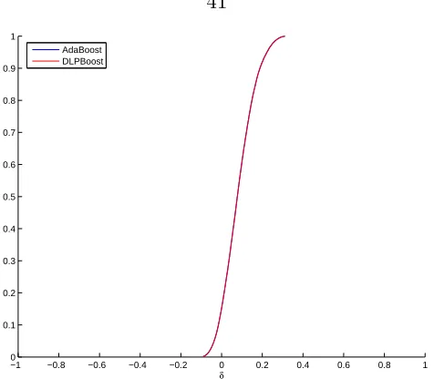
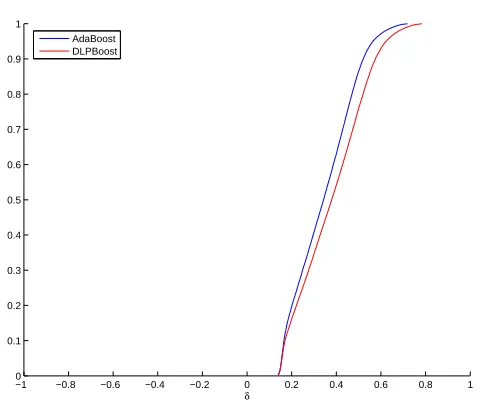
obtained by the two algorithms is reported in Figures 2.232.28
We can observe that the improvement in margins is signicant in some cases and very little in other cases. This improvement is inversely proportional to the increase in the errors. The two datasets Cancer and Sonar have a signicant change in the distribution and a large maximum change. DLPBoost performs signicantly worse on these two datasets.
2.7 Conclusions
−1 −0.8 −0.6 −0.4 −0.2 0 0.2 0.4 0.6 0.8 1 0
0.1 0.2 0.3 0.4 0.5 0.6 0.7 0.8 0.9 1
δ
AdaBoost DLPBoost
Figure 2.24: Margin Distribution on Sonar Dataset
−1 −0.8 −0.6 −0.4 −0.2 0 0.2 0.4 0.6 0.8 1
0 0.1 0.2 0.3 0.4 0.5 0.6 0.7 0.8 0.9 1
δ
AdaBoost DLPBoost
−1 −0.8 −0.6 −0.4 −0.2 0 0.2 0.4 0.6 0.8 1 0
0.1 0.2 0.3 0.4 0.5 0.6 0.7
δ
Figure 2.26: Margin Distribution on Ionosphere Dataset
−1 −0.8 −0.6 −0.4 −0.2 0 0.2 0.4 0.6 0.8 1
0 0.1 0.2 0.3 0.4 0.5 0.6 0.7 0.8 0.9 1
δ
AdaBoost DLPBoost
−1 −0.8 −0.6 −0.4 −0.2 0 0.2 0.4 0.6 0.8 1 0
0.1 0.2 0.3 0.4 0.5 0.6 0.7 0.8 0.9
δ
AdaBoost DLPBoost
Figure 2.28: Margin Distribution on Cancer Dataset
statistic of the margin is futile and would not lead to improvement in the performance of the algorithm.
Adaptive Estimation Under
Monotonicity Constraints
3.1 Introduction
The typical learning problem takes examples of the target function as input informa-tion and produces a hypothesis that approximates the target as an output. In this chapter, we consider a generalization of this paradigm by taking dierent types of information as input, and producing only specic properties of the target as output. Generalizing the typical learning paradigm in this way has theoretical and practi-cal merits. It is common in real-life situations that we would have access to heteroge-neous pieces of information, not only input-output data. For instance, monotonicity and symmetry properties are often encountered in modeling patterns of capital mar-kets and credit ratings [Abu-Mostafa 1995; 2001]. Input-output examples coming from historical data are but one of the pieces of information available in such appli-cations. It is also commonplace that we are not interested in learning the entirety of the target function, and would be better o focusing on only some specic properties of the target function of particular interest and achieving better performance in this manner. For instance, instead of trying to estimate an entire utility curve, we may be only interested in the threshold values at which the curve goes above or below a critical value.
is that the data is very expensive or time consuming to obtain. In many such cases, adaptive sampling is employed to get better performance with very small sample size [Cohn et al. 1994, MacKay 1992]. In this chapter, we will describe a new adaptive learning algorithm for estimating a threshold-like parameter from a monotonic func-tion. The algorithm works by adaptively minimizing the uncertainty in the estimate via its entropy. This, combined with a provably consistent learning algorithm, is able to achieve signicant improvement in performance over the existing methods.
3.1.1 Applications
This problem is very general in nature and appears in many dierent forms in Psy-chophysics [Palmer 1999, Klein 2001] , Standardized testing like the GRE [Baker 2001], adaptive pricing, and drug testing [Cox 1987]. In all these applications, there's a stimulus, and at each stimulus there is a probability of obtaining a positive response. This probability is known to be monotonically increasing.
The most popular application of these methods is in the eld of drug testing. It is known that the probability of a treatment curing a disease is monotonic in the level of dosage in the treatment, within a certain range. It is desirable to obtain a correct dose level which will induce a certain probability of producing a cure. The samples in this problem are very expensive and adaptive testing is generally the preferred approach.
Standardized tests, like the SAT and the GRE, use adaptive testing to evaluate the intelligence level of students. Item Response Theory [Lord 1980] models each question that is presented in the test as an item and for each item, the probability of a student correctly answering the question is monotonic in his intelligence. Each Item has a dierent diculty level, and the next item presented to the student is adaptively chosen based on his or her performance on the previous items. A student's GRE or SAT score is dened as a diculty level at which a student has a certain probability of correctly answering the questions.
sales goal.
All these applications have the common theme that the target is a monotonic function from which we can adaptively get Bernoulli samples which are otherwise expensive to obtain. In each of the cases, we are not interested in the whole target but only in a critical value of the input.
3.1.2 Monotonic Estimation Setup
Consider a family of Bernoulli random variables V(x) with parameters p(x) which
are known to be monotonic in x, i.e., p(x) ≤ p(y) for x < y. Suppose for X =
{x1, .., xM}, we have m(xi) independent samples of V(xi). We can estimate p(xi)
as the average number of positive responses yi. If the number of samples is small
then these averages will not necessarily satisfy the monotonicity condition. We will discuss the existing methods which take advantage of the monotonicity restriction on the estimation process and introduce a new regularized algorithm.
3.1.3 Threshold Function
We have a target function p:X →Y which is monotonically increasing. A threshold
functional θ maps a function p to X. The threshold function can take many forms,
the most common among them are:
Critical Value Crossing Functional. This is the most common form of the thresh-old. The problem here is to estimate the input value at which the monotonic function goes above a certain value. For example θ(h) =h−1(0.612) measures
the point at which the function crosses0.612.
is a xed known function and is usually monotonically non increasing. This kind of functional appears in the adaptive pricing problem, where the goal is to maximize expected prot. If the probability of a sale upon oering a discount rate of x isp(x), then the expected prot is given by θ(x) = (1−x)p(x).
3.1.4 Adaptive Learning Setup
In the adaptive learning setup, given an input point x ∈ X, we can obtain a noisy
output y = p(x) +²(x), where ² is a zero mean input dependent noise function.
For the scope of this chapter, Y = {0,1} and the noisy sample at x would be a
Bernoulli random variable with mean p(x), i.e., y|x = B(p(x)). This scenario is
common in various real-world situations in which we can only measure the outcome of the experiment (success or failure) and wish to estimate the underlying probability of success. For adaptive sampling, we are allowed to choose the location of the next sample based on the previous data samples and any prior knowledge that we might have. In the following sections, we will introduce existing and new methods to sample adaptively for monotonic estimation.
3.2 Existing Algorithms for Estimation under
Mono-tonicity Constraint
Most of the currently used methods employ a parametric estimation [Finney 1971, Wichmann and Hill 2001] technique for tting a monotonic function to the data. The main advantage of this method is the ease in estimation and the high regularization ability for small sample sizes, as there are only a small number of parameters to t.
3.2.1 Parametric Estimation
Parametric estimation is the most popular method used in practice. The method assumes a parametric form for the target and estimates the parameters using the data. This gives the entire target as the output. In most of the parametric methods, the target function is assumed to be coming from a 2-parameter family of functions.
The parameters are estimated from the data and the threshold or the threshold-like quantity can be computed from the inverse of the parametric function. The most commonly used methods for estimating the parameters are probit analysis [Finney 1971] and maximum likelihood [Watson 1971, Wichmann and Hill 2001]. In this thesis, we will use the maximum likelihood method with the two parameter logistic family [Hastie et al. 2001] as the model.
Flog ={f(x, a, b) = 1/(1 +e(x−a)/b)}
3.2.2 Non-Parametric Estimation
In the non-parametric approach (MonFit), [Barlow et al. 1972, Brunk 1955] the solu-tion is obtained by a maximum likelihood estimasolu-tion under the constraints that the underlying variables are monotonic. It is equivalent to nding the closest monotonic series in the mean square sense.
MonFit is an algorithm which solves the optimization problem
min
µ M
X
i=1
under the constraints
µi ≤µj ∀i≤j
The MonFit estimator always exists and is unique. It has a closed-form solution [Barlow et al. 1972]
ˆ
µ∗i = max
s≤i mint≥i Av(s, t) (3.2)
where
Av(s, t) =
P
im(xi)yi
P
im(xi)
The solution can be computed in linear time by the Pool Adjusted Vector Algo-rithm [Barlow et al. 1972]. The algoAlgo-rithm starts out with a pool of points, one for each of the design points xi. The value of the estimator for each pool is computed
as the average value of the points inside the pool. If there are two consecutive pools which violate the monotonicity restriction, then these pools are merged into one. This procedure is repeated until all consecutive pools obey the monotonicity restriction.
Theorem 1 Given examples from a family of Bernoulli random variables with mono-tonic probability, the MonFit estimate has a lower or equal mean square error than the naive estimate
Proof Let us consider the case when we have one example in each bin. We will denote the target aspi =p(xi)and assume that each bin has one sample, i.e.,m(xi) =
1. Suppose the rst pool of the MonFit estimate contains k points, then the partial
mean square error made in the rst pool for the MonFit case would be
e1mbt =
k
X
i=1
(¯y−pi)2
wherey¯=Pk
i=1yi is the average pooled value which is assigned to each bin in the
rst pool.
e1naive−e1mbt = 1 k
X
i,j=1
(yi−yj)2+
2 k
X
i=1
X
j=i+1
(pi−pj)(yj −yi) (3.3)
Now, since the rst k points were pooled, we have that
y1 ≥
y1+y2
2 ≥
y1+y2+y3
3 ≥. . .≥
Pk
i=1yi
k
From which we can conclude, that
y1 ≥y2 ≥y3 ≥. . .≥yk
p′
is are monotonic, therefore,
p1 ≤p2 ≤p3 ≤. . .≤pk
So, each term in equation (3.3) is non-negative. So, we have that e1
naive ≥e1mbt.
The mean square error would be the sum of the partial mean square errors in each pool, soenaive ≥embt
For the general case, when each bin has a weight wi = m(xi), we can do similar
calculation and get
e1naive−e1mbt = 1
k
k
X
i,j=1
wiwj(yi−yj)2+
2 k k X i=1 k X
j=i+1
wiwj(pi−pj)(yj−yi)
where, in this case,
e1mbt =
k
X
i=1
where
¯
y=
Pk
i=1wiyi
Pk
i=1wi
and
e1naive =
k
X
i=1
wi(yi −pi)2
and the ordering on y′
is still holds, so each term is again positive.
¤
Theorem 1 proves the advantage in enforcing the monotonicity constraint. The naive estimate is unbiased, and by enforcing the additional constraints the MonFit estimator becomes biased. However, the variance of the MonFit estimator is reduced. This result proves that overall, the increase in the bias is less than the corresponding decrease in the variance, making MonFit a better option for minimizing the mean square error.
The MonFit solution only gives the target values at the design points. To esti-mate the threshold, the function can be interpolated in any possible way. The most common approach is to interpolate it linearly in between the design points, although more sophisticated approaches are possible (like monotonic splines [Ramsay 1998]). We use linear interpolation because of its simplicity and the fact that we do not have any a priori knowledge to choose one over another. Theorem 2 proves the consis-tency property of the MonFit estimate with constant interpolation but it can also be extended to linear interpolation.
Theorem 2 Let f(x) be a continuous non-decreasing function on (a, b). Let {xn}be
a sequence of points dense in (a, b)with one observation made at each point. Let the
variance of the observed random variables be bounded. Let fˆn(x)be the estimate based
on the rst n observations, dened to be constant between observation points and
continuous from the left. If c > a and d < b, then
P
·
lim
n→∞cmax≤t≤d
¯ ¯
¯f(t)−fˆ(t) ¯ ¯ ¯= 0
¸
= 1
of both into one approach. We developed a regularized version of MonFit, which we call Bounded Jump Regression, that uses jump parameters to smoothen and regu-larize the MonFit solution. Bounded jump regression with a heuristic for parameter selection is used here for estimation in the hybrid estimation procedure.
3.3.1 Bounded Jump Regression
One of the main drawbacks of the non-parametric approach is that the solution it produces is a step function, which for many applications is non-smooth and tends to have a lot of at regions. Practically, this kind of behavior is unacceptable [Wichmann and Hill 2001]. In this section, we introduce a new approach to estimating the solution which introduces a parameter to the MonFit algorithm in order to make it smooth.
The non-parametric estimation technique solves a least squares regression problem under the monotonicity constraint. The monotonicity constraint ensures that the dierence between two consecutive estimates is positive. In this section we introduce a generalization of this problem where the dierence between two consecutive estimates is bounded above and below by certain parameters.
3.3.1.1 Denition
We dene the Bounded Jump Regression problem as follows
min
µ N
X
i=1
(µi−yi)2 (3.4)
Subject to the constraints that
whereµ0andµN+1are xed constants and{δi,∆i}Ni=1are parameters for the model.
3.3.1.2 Examples
Many of the regression problems can be expressed as a special case of the bounded jump regression problem. For regression of binomial probabilities which we are dealing with in this chapter, we x the boundary points µ0 = 0 and µN+1 = 1.
• When δi = −∞ and ∆i = ∞, the constraints are vacuous and the problem
reduces to normal mean squares regression.
• When δi = 0 and ∆i = ∞, the constraints enforce the monotonicity on µ′is ,
and so, the problem reduces to monotonic regression.
• When δi = 1/N + 1, there is only one feasible solution and so there is no
regression problem to solve.
3.3.1.3 Solving the BJR Problem
The BJR problem can be reduced to a quadratic optimization problem under box constraints by using suitable variable transformations. If we substitute
zi =
pi+1−pi−δi
1−PN
t=0δt
and
Ci =
∆i−δi
1−P
δt
and
Qij =min(N + 1−i, N + 1−j)
and
ynew
i =
i
X
t=1
Ã
¯ yt
1−PN
r=0δr
−δt
0≤z ≤C
and
zT1= 1
3.3.1.4 Special Cases
For the case when we have∆i =∞, the BJR can be reduced to monotonic regression
problem and hence can be solved in linear time. By using the transform
zi =
pi−Pit=1δt
1−PN
t=0δt
and
yinew = yi−
Pi
t=1δt
1−PN
r=0δr
The BJR reduces to
min
µ N
X
i=1
(zi−yinew)2 (3.6)
Subject to the constraints that
δ= 0
δ = 1/N
δ=−1
Figure 3.1: δ as a Complexity Parameter Controlling the Search Space
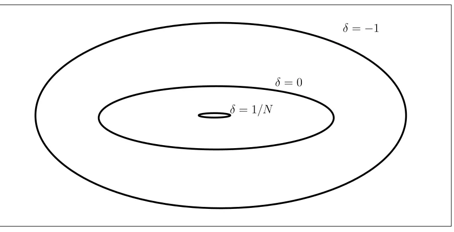
3.3.1.5 δ as a Complexity Parameter
Consider the case, when we have ∆i = ∞ , i.e., we're only bounding the minimum
jump between two consecutive bins, and δi =δ for alli. For the case when we have
δ = −∞, BJR reduces to normal regression and the set of feasible solution is the
entire RN plane (or if we are working with probabilities, it will be [0,1]N). As we
increase δ, the feasible region keeps shrinking. At δ = 0, the feasible region is the
set of all monotonic functions, and when δi = 1/N + 1, the feasible region contains
just one solution. So, δ can be seen as a measure of complexity of the solution space
and increasing delta will reduce the variance while increasing the bias. The number of independent parameters in the feasible region can also be considered as a function ofδ. Forδ =−∞, the number of independent parameters isN, and forδ = 1/N+ 1,
it is zero. This gives us a continuous control over the bias and variance trade-o.
δ =−∞ corresponds to the zero bias solution and δ = 1/N + 1 corresponds to the
we have a small number of examples. The jump parameter denotes the minimum value of the gradient of the target function. As we have seen in 3.3.1.5 , it co