Volume 2006, Article ID 91567, Pages1–10 DOI 10.1155/ASP/2006/91567
Adaptive DOA Estimation Using a Database of
PARCOR Coefficients
Eiji Mochida and Youji Iiguni
Department of Systems Innovation, Graduate School of Engineering Science, Osaka University, 1–3 Machikaneyama Toyonaka, Osaka 560-8531, Japan
Received 6 July 2005; Revised 8 March 2006; Accepted 23 March 2006
Recommended for Publication by Benoit Champagne
An adaptive direction-of-arrival (DOA) tracking method based upon a linear predictive model is developed. This method estimates the DOA by using a database that stores PARCOR coefficients as key attributes and the corresponding DOAs as non-key attributes. Thek-dimensional digital search tree is used as the data structure to allow efficient multidimensional searching. The nearest neighbour to the current PARCOR coefficient is retrieved from the database, and the corresponding DOA is regarded as the estimate. The processing speed is very fast since the DOA estimation is obtained by the multidimensional searching. Simulations are performed to show the effectiveness of the proposed method.
Copyright © 2006 Hindawi Publishing Corporation. All rights reserved.
1. INTRODUCTION
Estimation of the direction-of-arrival (DOA) for multiple sources plays an important role in the fields of radar, sonar, high-resolution spectral analysis, and communication sys-tems. A lot of high-resolution DOA estimation methods us-ing a linear array antenna [1–3] or usus-ing two identical sub-arrays [4] have been developed. The linear prediction (LP) method [5] is one of the well-known methods. The LP method characterises the bearing spectrum by the LP coeffi-cients, and provides a high-resolution spectrum even with a small number of antenna elements. However, the LP method requires to find local maxima (peak) of the bearing spectrum. The peak searching is computationally heavy, and thus the LP method is unsuitable for DOA tracking when DOAs change with time. Recently, Markov chain, Monte Carlo (MCMC) [6,7] method, and Gershman’s optimisation method [8,9] have been studied. MCMC method has high-resolution and Gershman’s method can be used for estimation of moving sources. These methods achieve a high estimation accru-acy, however their computational complexities are very large since optimisation problems need to be solved.
An adaptive DOA estimation method using a database has been proposed by one of the authors [10,11]. This meth-od uses autocorrelation coefficients as key attributes, and DOAs as non-key attributes. The nearest neighbour to the autocorrelation coefficients estimated from observation
sig-nals is retrieved from the database, and the corresponding DOA is regarded as the estimate. This method estimates the DOA by only a database retrieval method, and thus the pro-cessing speed is fast. However, the dimension of the key vec-tor increases in proportion to the number of antenna ele-ments. Therefore, as the number of antenna elements in-creases, the database size becomes larger and thus the pro-cessing speed is slower.
sL(t) s1(t)
θL θ1
d
x0(t) x1(t) xN 1(t)
w0 w1 wN 1
+ y(t)
Figure1: Distant wave source and linear array antenna.
using the Levinson-Durbin algorithm, retrieve a record with a key value nearest to the current key from the database, and use the corresponding DOA as the estimate. We then use the
k-d trie (k-dimensional digital search tree) [12] as the data structure to allow efficient multidimensional searching. The proposed method does not require exhaustive peak search-ing, and provides the estimation by only the database re-trieval method. Using this, we can reduce the dimension of the key vector to the number of signal sources even if the number of antenna elements is larger than the number of sig-nal sources. The size reduction of the key vector is extremely useful in decreasing search time.
2. DOA ESTIMATION PROBLEM AND LINEAR PREDICTION
2.1. DOA estimation problem
Consider L mutually uncorrelated signals with center fre-quency fc(wavelengthλc) arriving at a linear array antenna
ofN(N > L) inter-elements with distanced. We assume that the signals are narrow banded and the signal sources are far apart from the array. Let theith arriving signal at timet, the DOA, and the signal power besi(t),θi, andσi2, respectively.
Let the signal received by thejth element, the noise input on thejth antenna element, and the output of the array antenna bexj(t),nj(t), and y(t), respectively. The relation between
the signal sources and the linear array antenna is illustrated inFigure 1. The output vector from the array antenna is ex-pressed as
x(t)=x0(t),. . .,xN−1(t)T=
L
i=1 aθi
si(t) +n(t). (1)
Heren(t)=(n0(t),n1(t),. . .,nN−1(t))Tis anN-dimensional complex white noise vector, and (·)Tdenotes the transpose. We assume that noises{nj(t)}Nj=−01and signals{si(t)}Li=1are mutually uncorrelated.
In the case of the omnidirectional element, the response vectora(θi) is given by
aθi
=1,ejϕi,. . .,ejϕi(N−1)T (2)
withϕi=2πdcosθi/λc. We define the weight coefficient on
the jth array output aswj(j=0,. . .,N−1) and the weight
coefficient vector asw=(w0,w1,. . .,wN−1)T. The array out-put is then expressed as
y(t)=
N−1
j=0 ¯
wjxj(t)=wHx(t), (3)
where ¯(·) denotes the conjugation and (·)Hdenotes the Her-mitian transpose. We define the auto-correlation matrix of the output signalx(t) by
R=Ex(t)xH(t)=
L
i=1
σ2
ia
θi
aθi
H +σ2I
=
⎛ ⎜ ⎜ ⎜ ⎜ ⎜ ⎜ ⎜ ⎜ ⎜ ⎝
r0 r1 r2 · · · rN−1
¯
r1 r0 r1 rN−2 ¯
r2 r¯1 r0 ... ..
. . .. r1
¯
rN−1 · · · r¯1 r0
⎞ ⎟ ⎟ ⎟ ⎟ ⎟ ⎟ ⎟ ⎟ ⎟ ⎠ ,
(4)
whereIdenotes the identity matrix of sizeN, E[·] denotes the expectation operator, and σ2 denotes the noise power. The first term of the right-hand side of (4) is the signal term, of which rank is alwaysLif θi = θj (i = j), and the
sec-ond term is the noise term. The inclusion of the noise term guaranteesRto be full-rank ofN. Using the auto-correlation matrix, the output power is represented by
Ey(t)2=EwHx(t)2=wHRw. (5)
2.2. Linear prediction
When we setw0=1 in (3), we can have
x0(t)= −
N−1
j=1 ¯
wjxj(t) +y(t). (6)
When we predictx0(t) with a weighted linear combination of the output signals{xj(t)}Nj=−11, we can regard y(t) as the prediction error. We will determine the weight coefficients
{wj}Nj=−11so that the mean-square error is minimised. This is formulated as
min
w w
30 25 20 15 10 5 0 5
P
(
θ
)(
d
B
)
0 20 40 60 80 100 120 140 160 180 θ(deg)
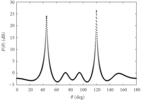
Figure 2: DOA estimation using the LP method for the case of (θ1,θ2)=(45◦, 120◦).
wherec=(1, 0, . . ., 0
N−1
)T. The constrained optimisation
prob-lem is easily solved by using the Lagrange multiplier method. The solution is given by
w∗=1,w∗1,. . .,wN∗−1 T
= 1
cHR−1cR
−1c. (8)
Here the weight coefficients{w∗j}Nj=−11 are referred to as the “LP coefficients.” It is here noted that the Capon spectrum is obtained by replacingcbya(θ) in (7).
The conventional LP method estimates the DOAs by lo-cally maximising the following bearing spectrum:
P(θ)= 1
aH(θ)w∗2. (9)
Figure 2shows an example of the bearing spectrum obtained by the LP method for the case of (θ1,θ2) = (45◦, 120◦). The extremely large peaks correspond with the DOAs, and the other small peaks are spurious. We have to perform the computationally expensive peak searching to find the two large peaks. The peak searching requiresO(NK) computa-tion steps, whereK is the number of bins. When the DOAs change with time, the peak searching has to be performed at each time. The iterative use of the peak searching requires a large amount of processing time. Thus the conventional LP method is unsuitable for adaptive DOA estimation.
3. DOA ESTIMATION USING A DATABASE RETRIEVAL SYSTEM
We have explained in Section 2that the peaks of the bear-ing spectrum are uniquely characterised by the LP coeffi-cients. We can thus estimate the DOAs by searching the near-est neighbour to the current LP coefficients in the database which stores pairs of the LP coefficients and the DOAs. This method can estimate the DOAs by only a database retrieval method. The processing speed is very fast, since exhaus-tive peak searching is not required. We first explain how to
construct the database, and then how to estimate the DOAs by database searching.
3.1. Database construction
3.1.1. Selection of model coefficients
We construct a database, which stores model coefficients as key attributes and DOAs as non-key attributes. The LP coeffi-cients{w∗j}Nj=−11seem to be good candidates for the model co-efficients. However, the LP coefficients are unsuitable as keys, because they take values in the range (−∞,∞). Instead of the LP coefficients, we use the PARCOR coefficients{ρj}N−1
j=1 which have a one-to-one correspondence to the LP coeffi-cients, as the keys.
We define thejth LP coefficient of orderiasw(ji)∗. When
the PARCOR coefficients{ρj}N−1
j=1 are given, the correspond-ing LP coefficients{w(jN−1)∗}Nj=−11are computed by using the recursion
w(ji)∗=w(ji−1)∗+ρiw¯(i−i−j1)∗ (j=1, 2,. . .,i). (10)
Here the recursion is initiated withi=2 and stopped when
i reaches the final valueN−1. On the other hand, when
{w(jN−1)∗}Nj=−11 are given, the corresponding PARCOR coef-ficients{ρj}N−1
j=1 are computed by using the recursion
w(ji−1)∗=
w(ji)∗−ρiw¯
(i)∗
i−j
1−ρi2 (j=1, 2,. . .,i−1) (11)
and the fact thatw(i−i−11)∗ =ρi−1. Here the recursion is initi-ated withi=N−1 and stopped whenireaches 2. Equations (10) and (11) show that there is a one-to-one relationship between the LP coefficients and the PARCOR coefficients. The PARCOR coefficients are more suitable as keys than the LP coefficients, because the PARCOR coefficients are robust against rounding errors and the absolute values are assured to be less than or equal to unity [13].
We see from (8) that the LP coefficients{w(jN−1)∗}Nj=−11 are uniquely computed from the auto-correlation matrix R. Consequently, the PARCOR coefficients{ρj}N−1
j=1 are also uniquely computed fromR. We also see from (4) thatRis ex-pressed as functions ofθi,σi2, andσ2. As a result,{ρj}Nj=−11is expressed as functions ofθi,σi2, andσ2. We define the
noise-free auto-correlation matrix by
R=R−σ2I=
L
i=1
σi2a
θi
aθi
H
, (12)
and then define the jth noise-free PARCOR coefficient
com-puted fromRbyρj. Sinceρj does not depend on the noise
powerσ2, it is a function of only (θ
i,σi2).
Let the rank ofRbep. WhenLDOAs are different from
ε2
0=r0
j=1, 2,. . .,N−1
Δj=r¯ j+
j
i=1
wi(j−1)∗r¯j−i
ρj=w(j)∗
j = −Δ j
ε2
j−1· · ·
ifρj2> α, then stop
ε2 j=ε2j−1
1−ρj2
i=1, 2,. . .,j−1
w(ij)∗=w
(j−1)∗
i +ρjw¯
(j−1)∗
j−i (A)
Algorithm1: Modified Levinson-Durbin algorithm.
Levinson-Durbin algorithm. To solve this problem, we de-velop a modified Levinson-Durbin (L-D) algorithm which recursively computes the LP and the PARCOR coefficients from the auto-correlation matrix by utilising the Toeplitz structure ofR. Using this algorithm, we can determine the noise-free LP coefficients and the noise-free PARCOR coeffi -cients of orderpfromR.
Algorithm 1 summarises the modified L-D algorithm. When applying the standard L-D algorithm to the noise-free auto-correlation matrixR of order p, the value of|ρp|
becomes unity during order update, and thenε2
p becomes
zero. We cannot compute the succeeding PARCOR coeffi -cients{ρj}N−1
j=p+1, because division by zero occurs in (A). For the solution, when |ρp| is larger than a thresholdα( 1),
we regard |ρp| as unity, terminate the update, and set the
succeeding noise-free PARCOR coefficients as zeros, that is,
ρp+1 = · · · = ρN−1 = 0. The reason for using this
proce-dure is that the value of|ρp|does not become exactly equal
to unity due to estimation errors. Using the modified L-D algorithm, we can obtainN−1 noise-free PARCOR coeffi -cients (ρ1,ρ2,. . .,ρp, 0, 0,. . ., 0
N−1−p
). Sincep≤L, we always have
ρj=0 forj=L+ 1,L+ 2,. . .,N−1. Zero coefficients do not
depend on the DOAs. Thus we use theLnoise-free PARCOR coefficients (ρ1,ρ2,. . .,ρL) as the database key.
3.1.2. Quantisation of data
We quantise the DOAsθi into θi(u) (u = 1, 2,. . .,U) and
the signal powersσ2
i intoσi2(v) (v = 1, 2,. . .,V), whereU
andV are the numbers of the DOA and signal power bins, respectively. Denoting the total number of the quantised data asM, we have
M=UL×VL. (13)
We put the quantisation step sizes of θi andσi2 asδθi and
δσ2
i, respectively. Asδθiandδσi2are smaller, the estimation
accuracy is higher while the database size is larger. We there-fore have to determine the values of δθi and δσi2 so that
a good tradeoff between the estimation accuracy and the database size is achieved. Whileθitakes values in the range
[0,π),σ2
i may take a very large value. The straightforward
quantisation of σi2 significantly increases the size ofV. We
have thus normalised the signal power σi2 with respect to
iσi2so that the normalised signal power is restricted to the
range (0, 1).
We define the noise-free auto-correlation matrices as
{R(m)}M
m=1, and the noise-free PARCOR coefficients corre-sponding to each of the M quantised data as {ρj(m)}M
m=1. We computeR(m) by using (12), and then computeρj(m)
fromR(m) by using the modified L-D algorithm. We further quantise the real and imaginary parts ofρj(m) to the integer
valuesz2j−1(m) andz2j(m) withbbits. Then we can have
z1(m),z2(m),. . .,z2L(m)
=QReρ1(m),QImρ1(m),
QReρ2(m),QImρ2(m),. . .,
QReρL(m),QImρL(m),
(14)
whereQis the output of the quantiser, and Re[x] and Im[x] denote the real and imaginary parts ofx, respectively. Note thatzj(m) takes value in the range [0, 2b−1].
3.1.3. Database storage
We define the PARCOR vector corresponding to the mth quantised data as
ρ(m)=z1(m),z2(m),. . .,z2L(m)
(m=1, 2,. . .,M) (15)
and the DOA vector corresponding toρ(m) as
θ(m)=θ1(m),θ2(m),. . .,θL(m)
(m=1, 2,. . .,M).
(16)
We successively store the pairs of{(ρ(m),θ(m))}M
m=1into the database. If the database has already stored the same PAR-COR vector as the current one, we delete it. We denote the number of data sets which are actually stored in the database asC. ThenCis much smaller thanMdue to the deletion of data sets.
3.2. DOA estimation
3.2.1. Estimation of PARCOR coefficients
We will present a method of estimating the auto-correlation matrixRfrom observation signalsxj(t) (j=0, 1,. . .,N−1).
by
Rt=
xtxtH+λxt−1xHt−1+λ2xt−2xHt−2+· · ·
1 +λ+λ2+· · ·
=λxt−1x
H
t−1+λxt−2xHt−2+λ2xt−3xHt−3+· · ·
1 +λ+λ2+· · ·
+ 1
1 +λ+λ2+· · ·xtx
H
t
=λRt−1+ (1−λ)xtxtH.
(17)
Here,λ(usually 0.95≤λ≤0.995) is a forgetting factor that controls the influence of the previous estimations, andRtis
the estimation of the auto-correlation matrix at timet. Un-fortunately, the recursive estimation using (17) does not pre-serve the Toeplitz structure ofR. We thus average the diago-nal elements ofRtto obtain the estimation ofrjas follows:
rj=
N−j l=1 Rt
l,l+j
N−j (j=0, 1,. . .,N−1), (18)
where (Rt)i,j denotes thei jth element ofRt. We next
sub-tract the noise powerσ2from the diagonal elements ofR
tto
estimate the noise-free auto-correlation matrixRas follows:
Rt=Rt−σ2I. (19)
Here the noise powerσ2is assumed to be known. It needs to be estimated a priori in the absence of source signals or needs to be estimated by using the eigenvalue decomposition of auto-correlation matrixR. We denote the estimation ofρj
asρj. We recursively calculate{ρj}N−1
j=1 fromRtby using the
modified L-D algorithm. In the same way as in the database construction, when|ρj|> α, we putρj+1 = · · · =ρN−1 =
0, and take the estimation of the PARCOR vector as
ρ=QReρ1,QImρ1, QReρ2,
QImρ2,. . .,QReρL,QImρL
≡z1,z2,. . .,z2L
.
(20)
3.2.2. Database retrieval
Mutidimensional searching is performed to retrieve the PAR-COR vector nearest toρfrom the database. More concretely, the PARCOR vectors lying in the hypercube {(z1,z2,. . .,
z2L)| |zj−zj| ≤D, j=1, 2,. . ., 2L}are retrieved from the
database. HereDdenotes the searching range which is a pos-itive integer number such that 0≤D≤2b−1. We take the
DOA vector corresponding to the retrieved PARCOR vec-tor as the DOA estimate, and denote the DOA estimation at time t as θt. When more than one PARCOR vector is
retrieved during the multidimensional searching, we select the PARCOR vector which minimises the Euclidean dis-tance2jL=1(zj−zj)2out of the retrieved ones. If no data
are retrieved, we take the previous estimationθt−1as the cur-rent estimationθt.
4. PERFORMANCE EVALUATION
We performed simulations for the cases ofL = 2 andL =
3 to evaluate the estimation performance of the proposed method.
4.1. DOA estimation for two signals
We constructed the database of L = 2, and estimated the DOAs of two moving sources.
4.1.1. Database construction
We consider the case where two signals arrive on the linear array antenna ofN=6 andd=λc/2. We quantise the DOA
by sampling cosθwith constant sampling interval 0.02, and quantise the normalised power with the constant sampling interval 0.25. Then we haveU=99 andV =4, and therefore
M=UL×VL=156816. We putb=8 andα=1−2/2b =
0.992 so that better estimation accuracy was obtained. We successively entered the data set{(ρ(m),θ(m))}M
m=1into the database. ThenC=22229 (=0.14×M), and the size of the database was about 776 (KB).
4.1.2. DOA estimation
We estimated the DOAs of two moving signals, where we put
σ12=40,σ22 =50, andσ2=1. Then we have SNR1 =16 dB and SNR2=17 dB. We have recursively estimatedRtby (17)
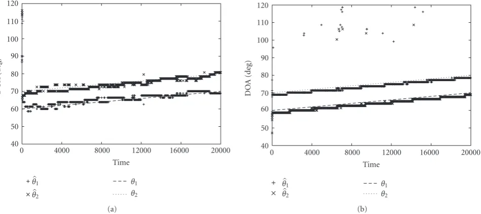
with λ = 0.995. As λis smaller, tracking capability is im-proved while stability of the estimations is lost. Therefore we have to make a tradeoffbetween tracking capability and sta-bility in the choice ofλ(usually 0.95≤λ≤0.995). Since the nonstationarity is weak in this case, we putλ = 0.995. We put the searching rangeD =10.Figure 3shows the results for the case whereθ1andθ2change by 1◦per 4000 snapshots starting from 60◦ and 70◦, respectively. For example, when the sampling frequency fsis 1.0 (MHz), the time intervalτ
isτ =1/ fs=1.0 (μs). Then the duration of 4000 snapshots
120 110 100 90 80 70 60 50 40
DO
A
(d
eg
)
0 4000 8000 12000 16000 20000
Time
θ1 θ2
θ1
θ2
(a)
120 110 100 90 80 70 60 50 40
DO
A
(d
eg
)
0 4000 8000 12000 16000 20000
Time
θ1 θ2
θ1
θ2
(b)
Figure3: Estimation results for two moving signals: (a) proposed method (b) LP method.
140 130 120 110 100 90 80 70 60 50
DO
A
(d
eg
)
0 4000 8000 12000 16000 20000
Time
θ1 θ2
θ1
θ2
(a)
140 130 120 110 100 90 80 70 60 50
DO
A
(d
eg
)
0 4000 8000 12000 16000 20000
Time
θ1 θ2
θ1
θ2
(b)
Figure4: Estimation results for two moving signals: (a) proposed method (b) LP method.
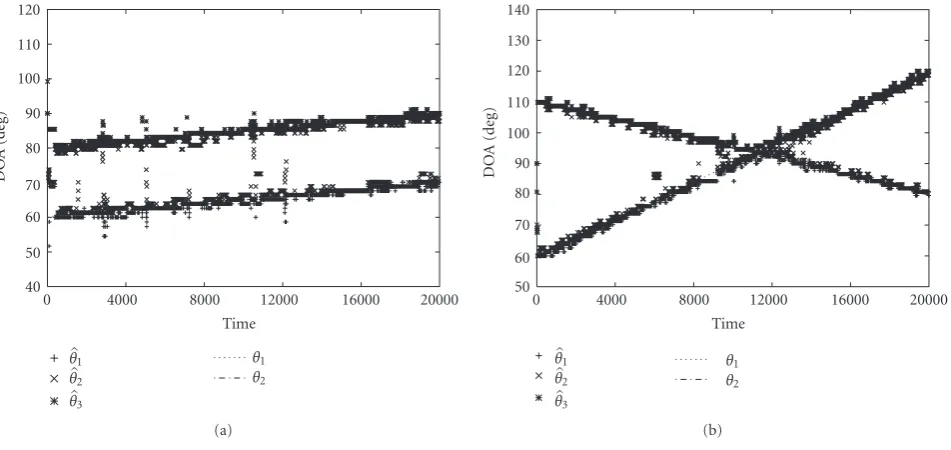
4.2. DOA estimation for three signals
We constructed the database of L = 3, and estimated the DOAs of three moving signals. We used the same quanti-sation step sizes as the previous ones. Then we had M =
62099136 andC=3821007 (=0.06×M). The database size was about 64 (MB).
4.2.1. DOA estimation
We putλ=0.995 andD=10 in the same way as in the pre-vious case. We estimated the DOAs of three moving signals
160 140 120 100 80 60 40
DO
A
(d
eg
)
0 4000 8000 12000 16000 20000
Time
θ1 θ2 θ3
θ1
θ2
θ3
(a)
160 140 120 100 80 60 40
DO
A
(d
eg
)
0 4000 8000 12000 16000 20000
Time
θ1 θ2 θ3
θ1
θ2
θ3
(b)
Figure5: Estimation results for three moving signals: (a) proposed method (b) LP method.
160 140 120 100 80 60 40
DO
A
(d
eg
)
0 4000 8000 12000 16000 20000
Time
θ1 θ2 θ3
θ1
θ2
θ3
(a)
160 140 120 100 80 60 40
DO
A
(d
eg
)
0 4000 8000 12000 16000 20000
Time
θ1 θ2 θ3
θ1
θ2
θ3
(b)
Figure6: Estimation results for three moving signals: (a) proposed method (b) LP method.
method sometimes fails due to the existence of the spurious peaks of the bearing spectrum, and the proposed method is much faster than the the LP method as shown later.
The proposed method requires a priori knowledge of the number of signalsL, because the database contents depend on the value ofL. Consequently,Lneeds to be estimated by using the model selection method such as Akaike informa-tion criteria (AIC) [14,15]. Fortunately, the proposed meth-od can well estimate the DOAs ofL signals using the data-base designed forL(>L) signals, although it fails whenL<L.
The reason is that estimation ofL signals is equivalent to the estimation ofLsignals whereL−L signals arrive at the same angle.
We will denote a database designed for theLsignals as
120 110 100 90 80 70 60 50 40
DO
A
(d
eg
)
0 4000 8000 12000 16000 20000
Time
θ1 θ2 θ3
θ1
θ2
(a)
140 130 120 110 100 90 80 70 60 50
DO
A
(d
eg
)
0 4000 8000 12000 16000 20000
Time
θ1 θ2 θ3
θ1
θ2
(b)
Figure7: Estimation results for two moving signals usingDB(3).
160 140 120 100 80 60 40
DO
A
(d
eg
)
0 4000 8000 12000 16000 20000
Time
θ1 θ2
θ1
θ2
θ3
Figure8: Estimation results for three moving signals usingDB(2).
4.3. Processing time
Table 1summarises the computation times of the proposed method and the LP method. In the proposed method, the values in the columns “Rt,” “ρj,” “k-d trie,” and “total” are
the time requirements of computingRt by (17), estimating
{ρj}L
j=1by using the modified L-D algorithm, multidimen-sional searching, and the total processing time, respectively. In the LP method, the values in the columns “w∗j” and “peak
searching” are the time requirements of estimating{w∗j}Nj=−11 by using the L-D algorithm and peak searching, respectively. In the proposed method, the database has been constructed a
priori, and it has been fixed during the estimation. Therefore, we do not need to include the time requirement of database construction in the processing time. All computations were done on an IBM PC/AT compatible computer with an Intel Pentium IV 2.4 GHz. The time of computingRtis the same
in both methods, that is, about 10.5μs per snapshot. When comparing the computation times excluding it, the proposed method with L = 2(L = 3) is about 50(30) times faster than the LP method. As the number of signal sourcesL in-creases, the database size gets larger and the processing time increases.
4.4. Determination of searching range
We have measured the estimation accuracy and the process-ing time for different values of the searchprocess-ing rangeD. We have evaluated the estimation accuracy by
J= 1
T
T
t=1
L
i=1 θt
i−θit
2
, (21)
whereθti denotes theith DOA at timet, andT denotes the
total snapshot.
Table1: Comparisons of processing time (per snapshot).
Simulation Proposed method (μs) LP method (μs)
Rt ρ
j
k-d trie Total Rt w∗j Peak searching Total
L=2 10.5 7.0 2.3 19.8 10.5 6.6 441.9 459.0
L=3 10.5 8.0 7.8 26.3 10.5 6.6 441.9 459.0
100000 10000 1000 100 10 1 0.1 J
0 2 4 6 8 10 12 14 16 18 20
Searching rangeD (a)
(b) (c)
(d) (e) (f)
Figure9: Estimation accuracy for different values ofD.
18 16 14 12 10 8 6 4 2 0
P
roc
essing
time
(
μ
s)
0 2 4 6 8 10 12 14 16 18 20
Searching rangeD (a)
(b) (c)
(d) (e) (f)
Figure10: Processing time for different values ofD.
increases as the value ofDis larger. There is a tradeoff be-tween the estimation accuracy and the processing time in de-terminingD. We thus judged from Figures9and10that the appropriate value is 10, and putD=10 in the previous sim-ulations.
5. CONCLUSION
We proposed the adaptive DOA estimation method using the database of PARCOR coefficients. In this method, the dimen-sion of key vector is equal to the number of signal sources and does not depend on the number of antenna elements. Thus the database size becomes relatively small and the processing speed is very fast. Although we found from simulation results that some erratic behaviours were observed due to quantisa-tions of PARCOR coefficients, the proposed method is much faster than the LP method and is robust against the spurious of the bearing spectrum.
REFERENCES
[1] J. Capon, “High-resolution frequency-wavenumber spectrum analysis,”Proceedings of the IEEE, vol. 57, no. 8, pp. 1408–1418, 1969.
[2] R. O. Schmidt, “Multiple emitter location and signal param-eter estimation,”IEEE Transactions on Antennas and Propaga-tion, vol. 34, no. 3, pp. 276–280, 1986.
[3] B. D. Rao and K. V. S. Hari, “Performance analysis of Root-Music,”IEEE Transactions on Acoustics, Speech, and Signal Pro-cessing, vol. 37, no. 12, pp. 1939–1949, 1989.
[4] R. Roy and T. Kailath, “ESPRIT - estimation of signal param-eters via rotational invariance techniques,”IEEE Transactions on Acoustics, Speech, and Signal Processing, vol. 37, no. 7, pp. 984–995, 1989.
[5] D. H. Johnson, “The application of spectral estimation meth-ods to bearing estimation problems,”Proceedings of the IEEE, vol. 70, no. 9, pp. 1018–1028, 1982.
[6] C. Andrieu, P. M. Djuri´c, and A. Doucet, “Model selection by MCMC computation,”Signal Processing, vol. 81, no. 1, pp. 19– 37, 2001.
[7] C. Andrieu and A. Doucet, “Joint Bayesian model selection and estimation of noisy sinusoids via reversible jump MCMC,”
IEEE Transactions on Signal Processing, vol. 47, no. 10, pp. 2667–2676, 1999.
[8] V. Katkovnik and A. B. Gershman, “Performance study of the local polynomial approximation based beamforming in the presence of moving sources,”IEEE Transactions on Antennas and Propagation, vol. 50, no. 8, pp. 1151–1157, 2002. [9] V. Katkovnik and A. B. Gershman, “A local polynomial
ap-proximation based beamforming for source localization and tracking in nonstationary environments,”IEEE Signal Process-ing Letters, vol. 7, no. 1, pp. 3–5, 2000.
[10] I. Setiawan, Y. Iiguni, and H. Maeda, “New approach to adap-tive DOA estimation based upon a database retrieval tech-nique,” IEICE Transactions on Communications, vol. E83-B, no. 12, pp. 2694–2701, 2000.
and clustering,”Digital Signal Processing, vol. 14, no. 6, pp. 590–613, 2004.
[12] J. A. Orenstein, “Multidimensional tries used for associative searching,”Information Processing Letters, vol. 14, no. 4, pp. 150–157, 1982.
[13] J. Makhoul, “Linear prediction: a tutorial review,”Proceedings of the IEEE, vol. 63, no. 4, pp. 561–580, 1975.
[14] M. Wax and T. Kailath, “Detection of signals by information theoretic criteria,”IEEE Transactions on Acoustics, Speech, and Signal Processing, vol. 33, no. 2, pp. 387–392, 1985.
[15] L. C. Godara, “Application of antenna arrays to mobile com-munications, part II: beam-forming and direction-of-arrival considerations,” Proceedings of the IEEE, vol. 85, no. 8, pp. 1195–1245, 1997.
Eiji Mochidareceived the B.E. and M.E. de-grees in communications engineering from Osaka University, Osaka, Japan, in 2001 and 2003, respectively, and the D.E. degree from Osaka University in 2006. He is now work-ing on hardware development for commu-nication systems at the Pixela Corporation, Osaka, Japan.