Fractional order Riccati differential equation: Analytical approximation and numerical results

R E S E A R C H

Open Access

Fractional-order Riccati differential equation:

Analytical approximation and numerical

results

Najeeb Alam Khan

_{, Asmat Ara}

_{and Nadeem Alam Khan}

*_{Correspondence:}

njbalam@yahoo.com 1_{Department of Mathematical}

Sciences, University of Karachi, Karachi, 75270, Pakistan Full list of author information is available at the end of the article

Abstract

The aim of this article is to introduce the Laplace-Adomian-Padé method (LAPM) to the Riccati differential equation of fractional order. This method presents accurate and reliable results and has a great perfection in the Adomian decomposition method (ADM) truncated series solution which diverges promptly as the applicable domain increases. The approximate solutions are obtained in a broad range of the problem domain and are compared with the generalized Euler method (GEM). The comparison shows a precise agreement between the results, the applicable one of which needs fewer computations.

Keywords: Adomian decomposition method (ADM); Mittag-Leffler function; Padé approximation; Riccati equation

1 Introduction

In recent years, it has turned out that many phenomena in biology, chemistry, acoustics, control theory, psychology and other areas of science can be fruitfully modeled by the use of fractional-order derivatives. That is because of the fact that a reasonable modeling of a physical phenomenon having dependence not only on the time instant but also on the prior time history can be successfully achieved by using fractional calculus []. Frac-tional differential equations (FDEs) have been used as a kind of model to describe several physical phenomena [–] such as damping laws, rheology, diffusion processes, and so on. Moreover, some researchers have shown the advantageous use of the fractional calculus in the modeling and control of many dynamical systems. Besides modeling, finding accurate and proficient methods for solving FDEs has been an active research undertaking. Exact solutions for the majority of FDEs cannot be found easily, thus analytical and numerical methods must be used. Some numerical methods for solving FDEs have been presented and they have their own advantages and limitations.

Many physical problems are governed by fractional differential equations (FDEs), and finding the solution of these equations have been the subject of many investigations in recent years. Recently, there have been a number of schemes devoted to the solution of fractional differential equations. These schemes can be broadly classified into two classes, numerical and analytical. The Adomian decomposition method [], homotopy perturba-tion method [–], homotopy analysis method [, ], Taylor matrix method [] and

Haar wavelet method [] have been used to solve the fractional-order Riccati differential equation. However, the convergence region of the corresponding results is rather small.

In this work, the nonlinear fractional-order Riccati differential equations will be ap-proached analytically by combining the Laplace transform, the Adomian decomposition method (ADM), and the Padé approximation. The Laplace-Adomian-Padé approximation was proposed by Tsai and Chen [] for solving Ricatti differential equations. The method was extended by Zenget al. [] to derive the analytical approximate solutions of fractional differential equations. Khanet al. [] applied the Laplace transformation coupled with the decomposition method in fractional order seepage flow and telegraph equations. We applied the idea of refs. [, ] for solving a fractional-order Riccati differential equation. The Laplace-Adomian-Padé method (LAPM) is illustrated by applications, and the results obtained are compared with those of the exact and numerical solutions by the generalized Euler method. Odibat and Momani [] derived the generalized Euler method that was developed for the numerical solution of initial value problems with Caputo derivatives.

2 Definitions and preliminaries

Caputo’s fractional derivative

Caputo’s fractional derivative of a functionf(t) is defined by

dα_f

dtα = 

(n–α)

t



(t–τ)n–α–f(n)(t)dt (n–  <α<n). ()

The Laplace transform to Caputo’s fractional derivative gives

L

dα

dtαf(t)

=sαF(s) – n–

m=

sα–m–f(m)() (n–  <α<n). ()

The Mittag-Leffler function and its generalized forms have played a special role in solv-ing the fractional differential equations. The so-called Mittag-Leffler function with two parametersEα,β(Z) was introduced by Agarwal []

Eα,β(Z) =

∞

j= Zj

(αj+β) (α> ,β> ). ()

Itskth derivative is given by []

E(αk,β)(Z) = ∞

j=

(j+k)!Zj

j!(αj+αk+β) (k= , , , , . . .). ()

We find it convenient to introduce the function

εk(t,a:α,β) =tαk+β–E(αk,β)

±atα_{. ()}

Its Laplace transform was evaluated by Podlubny []

_∞



e–stεk(t,a:α,β)dt=

k!sα–β (sα∓_a)k+

Hence

L– k!sα–β (sα_∓a)k+ =t

αk+β–_E(k)

α,β

±atα. ()

Another convenient property of εk(t,y:α,β), which has been used in this paper, is its simple fractional differentiation

Dλtεk(t,a:α,β) =εk(t,a:α,β–λ) (λ≺β). ()

3 Implementation of LAPM

Consider the fractional-order Riccati differential equation of the form

Dα_ty=P(t)y+Q(t)y+R(t), t> ,  <α≤ ()

subject to the initial condition

y() =k. ()

The nonlinear term in Eq. () isy_{andP(t),Q(t) andR(t) are known functions. Forα= ,}

the fractional-order Riccati equation converts into the classical Riccati differential equa-tion. Applying the Laplace transform on both sides of Eq. (),

LDα_ty=LP(t)y+LQ(t)y+LR(t). ()

Using the property of the Laplace transform, we get

sαL[y] –sα–y() =LP(t)y+LQ(t)y+LR(t). ()

Using the initial condition from Eq. (), the outcome is

sαL[y] –sα–k=L

P(t)y+LQ(t)y+LR(t). ()

Equation () can be written as

L[y] =k

s +



sαL

R(t)+ 

sαL

Q(t)y+ 

sαL

P(t)y. ()

The method assumes the solution as an infinite series:

y= ∞

n=

yn. ()

The nonlinearityy_{is decomposed as}

y= ∞

n=

whereAn=An(y,y,y,y, . . . ,yn) are the so-called Adomian polynomials given as

Substituting Eqs. () and () into Eq. (), the result is

L

Matching both sides of Eq. () yields the following iterative algorithm:

L[y] =

The aim is to study the mathematical behavior of the solution y(t) for different values ofα. By applying the inverse Laplace transform to both sides of Eq. (), the value ofy

is obtained. Substituting these values ofyandAinto Eq. (), the first componenty

is obtained. The other termsy,y,y, . . . . can be calculated recursively in a similar way

by Eqs. ()-(). The LAPM solution coincides with the Taylor series solution in the initial value case and diverges rapidly as the applicable domain increases. This goal can be achieved by forming Padé approximants, which have the advantage of manipulating the polynomial approximation into a rational function to gain more information about

y(t). It is well known that Padé approximants will converge on the entire real axis, ify(t) is free of singularities on the real axis. To consider the behaviors of a solution for different values ofα, we will take advantage of Eq. () available for  <α≤.

4 Test problems

In this section, we implement LAPM to the nonlinear fractional Riccati differential equa-tions. Two examples of nonlinear fractional Riccati differential equations are solved with real coefficients.

Test problem .Consider the nonlinear Riccati differential equation

Dα_t(y) =  + y(t) –y(t),  <α≤, ()

with the initial condition

The exact solution forα=  was found to be

First, applying the Laplace transform on both sides of Eq. (), we get

LDα t(y)

=L[] + L[y] –Ly. ()

Using the property of the Laplace transform, we obtain

sαL[y] –sα–y() =

s + L[y] –L

y. ()

Using the initial condition from Eq. (), it becomes

L[y] = 

Substituting Eqs. () and () into Eq. (), the result is

L

Matching both sides of Eq. () yields

L[y] =

Applying the inverse fractional Laplace transform to Eq. (), hence we can write it as

L[y] = s–

sα_{– }. ()

By applying the inverse Laplace transform to Eq. (), the valueyis obtained as

y=tαEα,+α

Now, considering the few terms ofy,

The first Adomian polynomialAis obtained from Eq. (), then we substituteyandA

in Eq. (). Evaluating the Laplace transform of the quantities on the right-hand side of Eq. () and then applying the inverse Laplace transform, the value ofycan be obtained.

The other termsy,y, . . . can be computed recursively in a similar calculation. By using

LAPM, a power series solution is essentially a truncated series solution. The LAPM so-lution coincides with the Maclaurin series of the exact soso-lution in the initial value case and diverges rapidly as the applicable domain increases. The next two components of the solution are

y= –

tα_{( + α)} (( +α))_{( + α)}–

tα_{( + α)} (( +α))_{( + α)}–

tα_{( + α)}

( +α)( + α)( + α)

– t

α_{( + α)}

(( +α))_{( + α)}–

tα_{( + α)}

( +α)( + α)( + α)

– t

α_{( + α)}

(( + α))_{( + α)}–· · ·, ()

y=

tα_{( + α)( + α)}

( +α)_{( + α)( + α)}+

tα_{( + α)( + α)}

( +α)_{( + α)( + α)}

+ t

α_{( + α)}

( +α)_{( + α)( + α)}+

tα_{( + α)( + α)}

( +α)_{( + α)( + α)}

+ t

α_{( + α)( + α)}

( +α)_{( + α)( + α)( + α)}+· · ·. ()

Therefore the truncated series solution obtained from LAPM is

y(t) =y+y+y+· · ·, ()

y(t) = t α

( +α)+ tα

( + α)+ tα

( + α)–

tα_{( + α)} (( +α))_{( + α)}

+ t

α

( + α)–

tα_{( + α)}

(( +α))_{( + α)}–· · ·. ()

The aim is to study the mathematical behavior of the result as the order of the fractional derivative changes. It was formally shown by Khanet al. [] that this goal can be achieved by forming Padé approximants [] which have the advantage of manipulating the poly-nomial approximation into a rational function to gain more information abouty(t). To consider the behavior of a solution of different values ofα, we will take advantage of Eq. () available for  <α≤ and consider the following three special cases.

Case I:Settingα=  in Eq. (), we reproduce the approximate solution obtained in Eq. (), given by the Taylor expansion ofy(t) att=  of the LAPM solution, as follows:

y(t) =t+t+ .t– .t– .t+Ot. ()

The Taylor expansion ofy(t) att=  of the exact solution () is

y(t) = .t+ .t+ .t– .t– .t+Ot. ()

is introduced. It is known that there exists the [_ML] Padé approximant which satisfies

∞

n= yn=

PL(t)

QM(t)

–OtL+M+=

L M +O

t. ()

By using Mathematica, the [_] Padé approximant gives that the rational approximation obtained from the solution in Eq. () is determined to be



 =

t+ .t– .t– .t· · ·+ .t

 – .t+ .t_{– .t}_{+· · ·– .×}–_t. ()

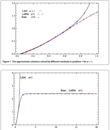
Figures - represent the comparisons between the exact solution, the LAM and the LAPM solutions in problem . They show that the LAM solutions diverge rapidly after

Figure 1 The approximate solutions solved by different methods in problem 1 forα= 1.

Table 1 Numerical results of the Riccati equation in problem 1

t GEMα= 1 LAPMα= 1 Exact solution Absolute error

y(t) y(t) y(t)

0.1 0.1000000000 0.1102952044 0.1102951969 7.5×10–9

0.2 0.2419000000 0.2419783394 0.2419767996 1.5×10–6

0.3 0.3580039000 0.3951442714 0.3951048487 0.00003942275

0.4 0.5167880007 0.5682377001 0.5678121663 0.00042553377

0.5 0.6934386 0.7588607194 0.7580143934 0.00084632599

Figure 3 The approximate curve of LAPM in problem 1 forα=1₂.

t= . However, they represent that the LAPM solution demonstrates a good convergence through the applicable domain. Table  shows the absolute errors of the LAPM solution in comparison with the exact and GEM solutions in problem .

Case II:Let us examine the caseα=_, the approximate solution obtained in Eq. () given by the Taylor expansion ofy(t) att=  has reproduced as

y(t) = .√t+ t+ .t _{– .t} · · ·_{. ()}

For simplicity, lett=z, then

y(z) = .z+ z+ .z–· · ·. ()

Calculating the [_] Padé approximation and recalling thatz=t_{, we obtain}



 =

.t/_{+ .t}/_{– .t}/_{· · ·+ .t}/

 – .t– .t_{– .t}· · ·_{.t}. ()

Figure  represents the LAPM solution in problem  forα=_.

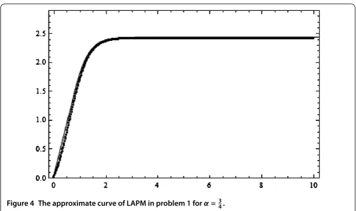
Case III:Here, takingα=_in Eq. (), the approximate solution has been replicated by

Figure 4 The approximate curve of LAPM in problem 1 forα=3₄.

Table 2 Numerical results of the Riccati equation in problem 1 forα= 1,1₂,3₄

t α=1

2GEM α=

1

2LAPM α=

3

4GEM α=

3

4LAPM α= 1LAPM

0.1 0.3568251903 0.3568031433 0.1934884034 0.1934012434 0.1102952044

0.2 0.9228652311 0.9228654512 0.4546091238 0.4546025138 0.2419783394

0.3 1.6341391963 1.6341391234 0.7840321022 0.7840324522 0.3951442714

0.4 2.2044414876 2.2044414576 1.1619801122 1.1619856232 0.5682377001

0.5 2.4004512311 2.4004476111 1.5438814841 1.5438814521 0.7588607194

0.6 2.0414276521 2.0414345521 1.8736212813 1.873658343 0.8840411201

0.7 2.4142176521 2.414888821 2.1129313512 2.112943562 1.0827124311

0.8 2.4142456641 2.4142478941 2.2602500123 2.260134223 1.2820124311

0.9 2.4142456047 2.4142455667 2.339920199 2.339134229 1.4740612089

1 2.4142410607 2.4142312137 2.3795146712 2.37935612 1. 6515902374

For simplicity, lett _{=z; then}

y(t) = .z+ .z– .z· · ·.×–z. ()

Calculating the [_] Padé approximants and recalling thatz=t, we achieve



 =

.t/– .t/+ .t/· · ·– .t/

 – .√t– .t+ .t/_{· · ·– ×}–_t/. ()

Figure  shows the LAPM solution in problem  forα=_.

Table  shows the results of the fractional Riccati equation in test problem  of the LAPM approximant solution in comparison with the different values ofα= ,_,_. The technique described above was translated into a Mathematica program and run on a Pentium- PC to investigate the effects of various values ofα= ,_,_ on the fractional Riccati differen-tial equation. The graphical results are in good agreement with the results of the exact solution.

Test problem .Consider the nonlinear Riccati differential equation

with the initial condition

y() = . ()

The exact solution [] was found to be

y(t) =e

t_{– }

et_{+ }. ()

First, applying the Laplace transform to both sides of Eq. (), we get

LDα t(y)

=L[] –Ly. ()

Using the property of the Laplace transform yields

sαL[y] –y() =

s–L

y. ()

Utilizing the initial conditions from Eq. (), it becomes

sαL[y] =

Substituting Eqs. () and () into Eq. (), the result is

L

Matching both sides of Eq. () yields the following iterative algorithm:

L[y] =

Applying the inverse fractional Laplace transform to Eq. (), hence the valueyis

y= tα

Substituting the value of y in Eq. (), the first Adomian polynomial A is obtained,

then substitutingyandAin Eq. () and proceeding in a similar way, the other terms y,y,y, . . . . can be computed recursively. The first twelve components of the solution are

Therefore the truncated series solution is obtained as

y(t) =y+y+y+· · ·+y ()

The plan is to study the mathematical performance of the solution of LAPM as the order of the fractional derivative changes. To consider the behavior of a solution of different values ofα, we will take advantage of the explicit formula Eq. () available for  <α≤ and consider the following three special cases.

Figure 5 The approximate solutions solved by different methods in problem 2 forα= 1.

It is known that there exists the [_ML] Padé approximant which satisfies

∞

n= yn=

PL(t)

QM(t)

–OtL+M+=

L M +O

t. ()

By using Mathematica, the Padé approximation gives that the truncated series obtained from the LAPM solution in Eq. () is determined to be



 =

t+_t₊  t+

 ,t+

 ,,t+



,,,t+ 

,,,,t

 +_t₊  t+

 ,t+

 ,t+



,,t+  ,,,t

. ()

From Figure , the presented result is in a good agreement with the exact result for

α = . Figure  represents the comparisons between the exact solution, the LAM, and the LAPM solutions for problem . It shows that the LAM solutions diverge rapidly after

t= . However, it represents that the LAPM solution demonstrates a good convergence through the applicable domain. Table  shows the absolute errors of the LAPM solution in comparison with the exact solution.

Case II:Here we examine the caseα=_in Eq. (), we replicate the approximate solu-tion obtained in Eq. () given by

y(t) = .√t– .t _{+ .t}· · ·_{+ .t}_{. ()}

For simplicity, lett_{=z; then}

y(t) = .z– .z+ .z· · ·+ .z. ()

Calculating the [_] Padé approximation and recalling thatz=t_{, we get}



 =

.t/_{+ .t}/_{– .t}/_{· · ·+ .t}/

Table 3 Comparison results of the Riccati equation in problem 2 forα= 1

t LAPMα= 1 Exact solution Absolute error

y(t) y(t)

1.0 0.7615941560 0.7615941560 0.01235728510×10–13

2.0 0.9640275801 0.9640275801 0.00524212251×10–12

3.0 0.9950547537 0.9950547537 0.00816114713×10–12

4.0 0.9993292997 0.9993292997 1.15746178216_×10–12

5.0 0.9999092043 0.9999092043 6.17826138530×10–11

6.0 0.9999877117 0.9999877117 4.55279023510×10–11

7.0 0.9999983377 0.9999983369 7.57246128510×10–10

8.0 0.9999997813 0.9999997749 6.33977368904×10–9

9.0 1.0000000063 0.9999999695 3.67962922016×10–8

10.0 1.0000001574 0.9999999958 1.61485463823×10–7

15.0 1.000000000 1.0000000000 0.00002076502676

20.0 1.0000000000 1.0000000000 0.00030117782151

25.0 1.0000000000 1.0000000000 0.00161702848408

30.0 1.0000000000 1.0000000000 0.00510751644687

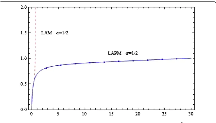
Figure 6 The approximate solutions solved by different methods in problem 2 forα=1 2.

Figure  shows the [

] Pade approximants ofy(t) in LAM and LAPM forα= 

. Figure 

illustrates the comparisons between the LAM solution and the LAPM solution in problem  forα=_.

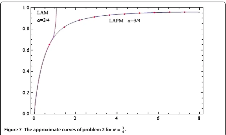
Case III:In this case we examine the LAPM whenα=_in Eq. ()

y(t) = .t_{– .t}_{+ .t} · · ·_{+ .t}_{. ()}

For simplicity, lett _{=z; then}

Figure 7 The approximate curves of problem 2 forα=3 4.

Table 4 Numerical results of the Riccati equation of problem 2 forα= 1,1₂,3₄

t α=1₂GEM α=1₂LAPM α=3₄GEM α=3₄LAPM α= 1LAPM

1 1.1283791670 0.69873925716 1.08806525252 0.73683666979 0.7615941560

2 0.8200613571 0.78565566383 0.88785292084 0.87018299629 0.9640275801

3 1.1896048240 0.82585713776 1.11809163866 0.91495001137 0.9950547537

4 0.7211473382 0.85006608584 0.84593506046 0.93590393958 0.9993292997

5 1.2627089888 0.86673312218 1.15537415211 0.94734255879 0.9999092043

6 0.5919620577 0.87923035124 0.79099259853 0.95361548723 0.9999877117

7 1.3249356376 0.88919590450 1.19828883587 0.95638359853 0.9999983377

8 0.4724965813 0.89752861875 0.72400539873 0.95643868318 0.9999997813

9 1.3489616923 0.90476369883 1.24172445342 0.95425989627 1.0000000063

10 0.4240319436 0.91123881947 0.65212406998 0.95020154024 1.0000001574

Calculating the [_] Padé approximation and recalling thatz=t_{, we get}



 =

.t/+ .×–t– .×–t/· · ·

– .×–t/

 + .×–t/– .×–√t· · ·

– .×–t/. ()

Figure  shows the [_] Padé approximants ofy(t) in LAPM forα=_. Table  shows the comparison results of the fractional Riccati equation in test problem  of the LAPM solution in comparison with the different values ofα= ,_,_. The procedure described above was translated into Mathematica program and run on a Pentium- PC to investigate the effects of special values ofα= ,_,_for the fractional Riccati differential equation.y(t) is evaluated up ton=  and plotted in Figure .

5 Conclusions

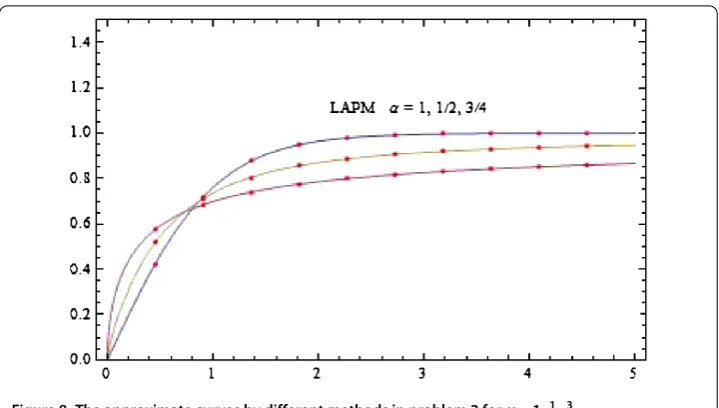
Figure 8 The approximate curves by different methods in problem 2 forα= 1,1₂,3₄.

to catch critical points at which a sudden divergence or bifurcation starts. Therefore, high accuracy solutions are always needed. Here, we have implemented the Adomian decom-position method coupled with the Laplace transformation and the Padé approximation on the Ricatti differential equation with fractional order. From the test problems considered here, it can be easily seen that LAPM obtains results as accurate as possible. Thus, it can be concluded that the LAPM methodology is very dominant and efficient in finding ap-proximate solutions, and comparison has been made with GEM. This paper can be used as a standard paradigm for other applications. The results of LAPM have been compared with exact solutions and ref. [] forα= .

Competing interests

The authors declare that they have no competing interests.

Authors’ contributions

The authors have equal contributions and they have approved the final version of the manuscript.

Author details

1_{Department of Mathematical Sciences, University of Karachi, Karachi, 75270, Pakistan.}2_{Department of Mathematical}

Sciences, Federal Urdu University Arts, Science and Technology, Karachi, 75300, Pakistan.

Acknowledgements

The authors would like to express their sincere gratitude to the referees for their careful assessment and suggestions regarding the initial version of the manuscript. The author Najeeb Alam Khan is highly thankful and grateful to the Dean of Faculty of Sciences, University of Karachi, Karachi-75270, Pakistan for facilitating this research work.

Received: 8 January 2013 Accepted: 29 May 2013 Published: 26 June 2013

References

1. Podlubny, I: Fractional Differential Equations. Academic Press, New York (1999)

2. Khan, NA, Jamil, M, Ara, A, Das, S: Explicit solution of time-fractional batch reactor system. Int. J. Chem. React. Eng.9, Article ID A91 (2011)

3. Feliu-Batlle, V, Perez, R, Rodriguez, L: Fractional robust control of main irrigation canals with variable dynamic parameters. Control Eng. Pract.15, 673-686 (2007)

4. Podlubny, I: Fractional-order systems and controllers. IEEE Trans. Autom. Control44(1), 208-214 (1999)

5. Garrappa, R: On some explicit Adams multistep methods for fractional differential equations. J. Comput. Appl. Math.

229, 392-399 (2009)

6. Jamil, M, Khan, NA: Slip effects on fractional viscoelastic fluids. Int. J. Differ. Equ.2011, Article ID 193813 (2011) 7. Abbasbandy, S: Homotopy perturbation method for quadratic Riccati differential equation and comparison with

8. Odibat, Z, Momani, S: Modified homotopy perturbation method: application to quadratic Riccati differential equation of fractional order. Chaos Solitons Fractals36(1), 167-174 (2008)

9. Khan, NA, Ara, A, Jamil, M: An efficient approach for solving the Riccati equation with fractional orders. Comput. Math. Appl.61, 2683-2689 (2011)

10. Aminkhah, H, Hemmatnezhad, M: An efficient method for quadratic Riccati differential equation. Commun. Nonlinear Sci. Numer. Simul.15, 835-839 (2010)

11. Abbasbandy, S: Iterated He’s homotopy perturbation method for quadratic Riccati differential equation. Appl. Math. Comput.175, 581-589 (2006)

12. Cang, J, Tan, Y, Xu, H, Liao, SJ: Series solutions of non-linear Riccati differential equations with fractional order. Chaos Solitons Fractals40, 1-9 (2009)

13. Tan, Y, Abbasbandy, S: Homotopy analysis method for quadratic Riccati differential equation. Commun. Nonlinear Sci. Numer. Simul.13, 539-546 (2008)

14. Gülsu, M, Sezer, M: On the solution of the Riccati equation by the Taylor matrix method. Appl. Math. Comput.176(2), 414-421 (2006)

15. Li, Y, Hu, L: Solving fractional Riccati differential equations. In: Third International Conference on Information and Computing Using Haar Wavelet. IEEE (2010). doi:10.1109/ICIC.2010.86

16. Tsai, P, Chen, CK: An approximate analytic solution of the nonlinear Riccati differential equation. J. Franklin Inst.347, 1850-1862 (2010)

17. Zeng, DQ, Qin, YM: The Laplace-Adomian-Pade technique for the seepage flows with the Riemann-Liouville derivatives. Commun. Frac. Calc.3, 26-29 (2012)

18. Khan, Y, Diblik, J, Faraz, N, Smarda, Z: An efficient new perturbative Laplace method for space-time fractional telegraph equations. Adv. Differ. Equ.2012, Article ID 204 (2012)

19. Odibat, Z, Momani, S: An algorithm for the numerical solution of differential equations of fractional order. J. Appl. Math. Inform.26, 15-27 (2008)

20. Agarwal, RP: A propos d’une note de M. Pierre Humbert. C. R. Acad. Sci. Paris236(21), 2031-2032 (1953) 21. Khan, NA, Jamil, M, Ara, A, Khan, NU: On efficient method for system of fractional differential equations. Adv. Differ.

Equ.2011, Article ID 303472 (2011)

22. Baker, GA: Essentials of Padé Approximants. Academic Press, London (1975)

doi:10.1186/1687-1847-2013-185