R E S E A R C H
Open Access
A posteriori truncated regularization
method for identifying unknown heat source
on a spherical symmetric domain
Fan Yang
*, Miao Zhang, Xiao-Xiao Li and Yu-Peng Ren
*Correspondence:
[email protected] School of Science, Lanzhou University of Technology, Lan Zhou, 730050, China
Abstract
In this paper, we mainly consider the inverse problem for identifying the unknown heat source in spherical symmetric domain. We propose a truncation regularization method combined with ana posterioriregularization parameter choice rule to deal with this problem. The Hölder type convergence estimate is obtained. Numerical results are presented to illustrate the accuracy and efficiency of this method.
Keywords: identifying the unknown source; ill-posed problem; regularization method;a posterioriparameter choice rule; spherical symmetric domain
1 Introduction
Identifying the unknown heat source in a parabolic partial differential equation from the over-specified data plays an important role in applied mathematics, physics and engi-neering. These problems are widely encountered in the modeling of physical phenomena. A typical example is groundwater pollutant source estimation in cities with large popula-tion []. Now many scholars have used different methods to identify various types of heat sources. In [, ], the authors used the method of fundamental solutions and radial ba-sis functions to identify the unknown heat source. In [, ], the authors used the Fourier truncation method and the wavelet dual least squares method to identify the spatial vari-able heat source. In [], the authors used the simplified Tikhonov method to identify the spatial variable heat source. In [, ], the authors determined the heat source which de-pends on one variable in a bounded domain using the boundary-element method and an iterative algorithm. In [], the authors identified the heat source which depends only on time variable using the Lie-group shooting method (LGSM). In [], the authors used the truncation method based on Hermite expansion to identify the unknown source in a space fractional diffusion equation. In [], the authors identified the point source with some point measurement data. In [], the authors proved the existence and uniqueness for identifying the heat source which depends only on time variable. In [], the authors used the variational method to identify the heat source which has the formF(x,t). In [], the authors used the variational method to identify the heat source which has the form of
F(x,t) =F(x)H(t) for the variable coefficient heat conduction equation. As far as we know, most of the researches on heat source identification problem mainly concentrated on one-dimensional case. But for a high one-dimensional case, there are few research results. In [],
the authors used the spectral method to identify the heat source in a columnar symmet-ric domain. In [], the authors used the spectral method to identify the heat source in a spherically symmetric parabolic equation. But the regularization parameters is selected by thea priorirule. There is a defect for anya priorimethod,i.e., thea priorichoice of the regularization parameter depends seriously on thea prioriboundEof the unknown solution. However, thea prioriboundEcannot be known exactly in practice, and work-ing with a wrong constantEmay lead to a badly regularized solution. In this paper, we not only give thea posteriorichoice of the regularization parameter which depends only on the measurable data, but also we give some different examples to compare the effective-ness between theposteriorchoice rule and thepriorichoice rule. Moreover, we find the truncation regularization method is better than the other regularization methods, such as Tikhonov regularization and the quasi-boundary value regularization method for solving this problem. To the best of the authors’ knowledge, there are few papers to choose the regularization parameter under thea posteriorirule for this problem.
In this paper, we consider the following heat source identification problem in spherical symmetric domain: there must be measurement errors, and we assume the measured data functionϕδ(r)∈ L[,r
;r], and it satisfies
ϕ(·) –ϕδ(·)≤δ, ()
whereδ> is the measurable error level.
Using the separation variable method, we get the solution of problem () as follows:
u(r,t) =
whereψn(r) defined as follows are the characteristic functions:
Usingu(r,T) =ϕ(r), we obtain
ϕ(r) =
∞
n= fn
T
e–(nrπ)
(T–τ) dτ
ψn(r). ()
Due to the mean value theorem of integrals, we obtain
ϕ(r) =
∞
n= fn
Te–(nrπ) (T–t
n)
ψn(r), <tn<T. ()
Define the operatorK:f(·)→ϕ(·), then we have
ϕ(r) =Kf(r) =
∞
n=
Te–(nrπ)(T–tn)
(f,ψn)ψn. ()
It is easy to see thatK is a linear compact operator, and the singular values{σn}∞n=ofK
satisfy
σn=Te–(
nπ
r)(T–tn)
()
and
(ϕ,ψn) = (f,ψn)Te–(
nπ
r)(T–tn)
, ()
i.e.,
(f,ψn) =σn–(ϕ,ψn). ()
So
f(r) =K–ϕ(r) =
∞
n=
σn–ϕ(r),ψn(r)ψn(r). ()
From equation (), we can seeσn–→ ∞(n→ ∞). Thus, the exact data functionϕ(r) must decrease rapidly. But the measured data functionϕδ(r) only belongs toL[,r
;r],
we cannot expect it has the same decay rate inL[,r
;r]. Thus the problem () is
ill-posed. It is impossible to solve this problem using a classical method. We will use the truncated regularization method to deal with the ill-posed problem. Before doing that, we impose ana prioribound on the unknown heat source,i.e.,
f(·)Hp(,π)≤E, p> , ()
where E> is a constant and · Hp(,π) denotes the norm in Sobolev space which is
defined as follows:
f(·)Hp(,π):=
∞
n=
+npf(·),ψn(·)
This paper is organized as follows. In Section , under thea posterioriparameter choice rule, we give the convergence error estimate. In Section , three numerical examples are used to verify the effectiveness for the proposed method. In Section , the conclusion of this paper is given.
2 Main result
From (), we define
fNδ=PN
fδ(r)= N
n=
σn–ϕnδψn ()
as the regularized solution of (), wherePN:L[,r;r]→span{ψn|n≤N}is the rectan-gular projection,
ϕnδ=ϕδ,ψn
, n= , , . . . ()
is the Fourier coefficient ofϕδ(r). Due to the discrepancy principle, we consider ana pos-terioriregularization parameter choice rule as follows:
(I–PN)ϕδ≤τ δ<(I–PN–)ϕδ, ()
whereτ> is a constant,Iis an identity operator inL[,r ;r].
Let
ρN=(I–PN)ϕδ. ()
According to the following lemma, we know there exists an unique solution for ().
Lemma Forδ> ,the functionρN satisfies:
(a) ρN is a continuous function;
(b) limN→+ρN=ϕδ; (c) limN→+∞ρN = ;
(d) ρN is a strictly decreasing function over(,∞).
Lemma ([, ]) As n≥,we obtain
c
nπ ≤σn≤ c
nπ, ()
where c,care constants.
Lemma Assume conditions()and()hold.N is taken as the solution of().Then we have
N(δ)≤c
(τ– )δ E
–
p+
, ()
where c:=π –
p+c
Proof Using (), we have
On the other hand,
(I–PN–)ϕ=(I–PN–)ϕδ– (I–PN–)
This completes the proof of Lemma .
Lemma If the regularized solution is given by(),we have
fδ
Proof Due to (), we obtain
fNδ(δ)(·) –fN(δ)(·)=
Lemma Suppose conditions()and()hold.f(r)given by()is the exact solution of
(),then we obtain
f(·) –fN(δ)(·)≤c(τ+ )
This completes the proof of Lemma .
Now we give the convergent error estimate between the exact solution and the regular-ized solution.
Theorem f(r)given by()is the exact solution of(),fδ
N given by()is the regularized
solution of().The regularization parameter is given by().So we have
f(·) –fδ
Proof Using the triangle inequality, () and (), we have
f(·) –fNδ(δ)(·)=f(·) –fN(δ)(·) +fN(δ)(·) –fNδ(δ)(·)
3 Numerical experiments
In this section, three numerical examples are used to illustrate the usefulness of proposed method. Moreover, the comparisons of numerical effectiveness between thea posteriori
parameter choice () and thea prioriparameter choice rule which is obtained byN= [(Eδ)p+] in [] are also considered. The measurable data is given as follows:
ϕδ(r) =ϕ+εrandnsize(ϕ), ()
where
ϕ=ϕ(r), . . . ,ϕ(rn)
T
, ri= (i– )r,r=
r
n– ,i= , , . . . ,n. ()
The total noise levelδcan be measured in the sense of the root mean square error (RMSE) as follows:
δ=ϕδ–ϕL=
n
n
i=
ϕi–ϕiδ
. ()
To show the accuracy of numerical solution, the approximateL error is computed as follows:
ea=f(r) –fNδ(r)L,
and the approximate relative error inLnorm is denoted by
er=f
(r) –fNδ(r)
f(r) .
It is difficult to find an exact solution for problem () in our numerical experiment. We first give the heat sourcef(r) and solve the following direct problem:
⎧ ⎪ ⎪ ⎪ ⎪ ⎪ ⎨ ⎪ ⎪ ⎪ ⎪ ⎪ ⎩
ut–rur–urr=f(r), <t<T, <r<r,
u(r, ) = , ≤r≤r, u(r,t) = , ≤t≤T, u(,t) = , <t<T.
()
Then we useu(r,T) =ϕ(r) and () to obtain the exact dataϕ(r) and the noise dataϕδ(r), respectively. Finally, we solve the inverse problem to obtain the regularization solution
fδ
N(δ)(r). In the following three numerical examples, we takeT= andr=π.
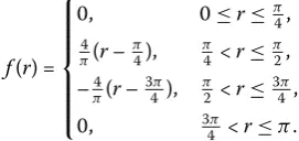
Example Consider a piecewise smooth heat source:
Example Consider the following discontinuous function:
f(r) =
Firstly, we use Examples and Examples to compare the numerical effects among the truncate regularization method, the Tikhonov regularization method and quasi-boundary value regularization method under thea posteriorichoice rule. The numerical results is shown in Tables and . The Tikhonov regularization solution of problem () is given as follows:
where <α< is the regularization parameter.
Through modifying the final value conditionu(r,T) =ϕ(r), we solve the following
prob-whereμis the regularization parameter. Then we obtain the quasi-boundary value solu-tion of problem () as follows:
fμδ(r) =
Tables and gives the comparisons of the numerical results of the truncate regulariza-tion method, the Tikhonov regularizaregulariza-tion method and the quasi-boundary regularizaregulariza-tion method under thea posteriorichoice rule for differentε. From Tables and , we can see that the effectiveness of the truncate regularization method in the present paper is better than the other regularization methods.
Table 1 Numerical results for differentεunder ana posteriorichoice rule for three regularization methods about Examples 1
ε 0.05 0.01 0.005 0.001 0.0005 0.0001
Truncate ea 0.0697 0.0376 0.0243 0.0118 0.0082 0.0035
er 0.0593 0.0320 0.0207 0.0101 0.0070 0.0030
Tikhonov ea 0.1024 0.0407 0.0277 0.0152 0.0065 0.0034
er 0.0871 0.0346 0.0236 0.0129 0.0056 0.0029
Quasi-boundary ea 0.6363 0.1518 0.0437 0.0160 0.0107 0.0043
er 0.5414 0.1291 0.0372 0.0136 0.0091 0.0037
Table 2 Numerical results for differentεunder ana posteriorichoice rule for three regularization methods about Examples 2
ε 0.05 0.01 0.005 0.001 0.0005 0.0001
Truncate ea 0.0972 0.0521 0.0304 0.0241 0.0226 0.0139
er 0.2392 0.1283 0.0749 0.0594 0.0557 0.0341
Tikhonov ea 0.1295 0.0871 0.0361 0.0273 0.0243 0.0378
er 0.3178 0.2143 0.0889 0.0672 0.0598 0.0930
Quasi-boundary ea 0.7800 0.2036 0.0566 0.0539 0.0482 0.0393
er 1.9194 0.5011 0.1393 0.1327 0.1186 0.0967
Figure 1 The comparison of numerical effects between the exact solution and its computed approximations forp= 1 with Examples 1: (a)ε= 0.001, (b)ε= 0.0001.
Figure 2 The comparison of numerical effects between the exact solution and its computed approximations forp= 1 with Examples 2: (a)ε= 0.001, (b)ε= 0.0001.
Figure 3 The comparison of numerical effects between the exact solution and its computed approximations forp= 1 with Examples 3: (a)ε= 0.001, (b)ε= 0.0001.
4 Conclusion
Acknowledgements
The authors would like to thanks the editor and the referees for their valuable comments and suggestions that improve the quality of our paper. The work is supported by the National Natural Science Foundation of China
(11561045,11501272) and the Doctor Fund of Lan Zhou University of Technology.
Competing interests
The authors declare that they have no competing interests.
Authors’ contributions
All authors contributed equally and significantly in writing this article. All authors read and approved the final manuscript.
Publisher’s Note
Springer Nature remains neutral with regard to jurisdictional claims in published maps and institutional affiliations.
Received: 5 January 2017 Accepted: 12 July 2017 References
1. Li, G, Tan, Y, Cheng, J, Wang, X: Determining magnitude of groundwater pollution sources by data compatibility analysis. Inverse Probl. Sci. Eng.14, 287-300 (2006)
2. Micrzwiczak, M, Kolodziej, JA: Application of the method of fundamental solutions and radical basis functions for inverse tranyient heat source problem. Commun. Comput. Phys.181, 2035-2043 (2010)
3. Ahmadabadi, MN, Arab, M, Ghaini, FMM: The method of fundamental solutions for the inverse space-dependent heat source problem. Eng. Anal. Bound. Elem.33, 1231-1235 (2009)
4. Dou, FF, Fu, CL, Yang, FL: Optimal error bound and Fourier regularization for identifying an unknown source in the heat equation. J. Comput. Appl. Math.230, 728-737 (2009)
5. Dou, FF, Fu, CL: Determining an unknown source in the heat equation by a wavelet dual least squares method. Appl. Math. Lett.22, 661-667 (2009)
6. Yang, F, Fu, CL: A simplified Tikhonov regularization method for determining the heat source. Appl. Math. Model.34, 3286-3299 (2010)
7. Farcas, A, Lesnic, D: The boundary-element method for the determination of a heat source dependent on one variable. J. Eng. Math.54, 375-388 (2006)
8. Johansson, T, Lesnic, D: Determination of a spacewise dependent heat source. J. Comput. Appl. Math.209, 66-80 (2007)
9. Liu, CH: A two-stage LGSM to identify time-dependent heat source through an internal measurement of temperature. Int. J. Heat Mass Transf.52, 1635-1642 (2009)
10. Zhao, ZY, Xie, O, You, L, Meng, ZH: A truncation method based on Hermite expansion for unknown source in space fractional diffusion equation. Math. Model. Anal.19, 430-442 (2014)
11. Badia, ELA, Ha-Duong, T, Hamdi, A: Identification of a point source in a linear advection-dispersion-reaction equation: application to a pollution source problem. Inverse Probl.21, 1121-1136 (2005)
12. Ismailov, MI, Kanca, F, Lesnic, D: Determination of a time-dependent heat source under nonlocal boundary and integral overdetermination conductions. Appl. Math. Comput.218, 4138-4146 (2011)
13. Ma, YJ, Fu, CL, Zhang, YX: Identification of an unknown source depending on both time and space variables by a variational method. Appl. Math. Model.36, 5080-5090 (2012)
14. Hasanov, A: Identification of spacewise and time dependent source terms in 1D heat conduction equation from temperature measurement at a final time. Int. J. Heat Mass Transf.55, 2069-2080 (2012)
15. Cheng, W, Ma, YJ, Fu, CL: Identifying an unknown source term in radial heat conduction. Inverse Probl. Sci. Eng.20, 335-349 (2012)
16. Cheng, W, Zhao, LL, Fu, CL: Source term identification for an axisymmetric inverse heat conduction problem. Appl. Math. Lett.26, 387-391 (2013)
17. Liu, JJ, Yamamoto, M: A backward problem for the time-fractional diffusion equation. Appl. Anal.89, 1769-1788 (2010)