R E S E A R C H
Open Access
Delay-aware tree construction and
scheduling for data aggregation in duty-cycled
wireless sensor networks
Duc Tai Le
1, Taewoo Lee
2and Hyunseung Choo
1,2*Abstract
Data aggregation is one of the most essential operations in wireless sensor networks (WSNs), in which data from all sensor nodes is collected at a sink node. A lot of studies have been conducted to assure collision-free data delivery to the sink node, with the goal of minimizing aggregation delay. The minimum delay data aggregation problem gets more complex when recent WSNs have adopted the duty cycle scheme to conserve energy and to extend the network lifetimes. The reason is that the duty cycle yields a notable increase of communication delay, beside a reduction of energy consumption, due to the periodic sleeping periods of sensor nodes. In this paper, we propose a novel data aggregation scheme that minimizes the data aggregation delay in duty-cycled WSNs. The proposed scheme takes the sleeping delay between sensor nodes into account to construct a connected dominating set (CDS) tree in the first phase. The CDS tree is used as a virtual backbone for efficient data aggregation scheduling in the second phase. The scheduling assigns the fastest available transmission time for every sensor node to deliver all data collision-free to the sink. The simulation results show that our proposed scheme reduces data aggregation delay by up to 72% compared to previous work. Thanks to data aggregation delay reduction, every sensor node has to work shorter and the network lifetime is prolonged.
Keywords: Data aggregation scheduling, Collision-free, Duty cycle, Wireless sensor networks
1 Introduction
Wireless sensor networks (WSNs) are generally composed of a large number of sensor nodes cooperating with each other to conduct various services, such as monitoring a disaster area in environmental services, detecting event on a barrier in military surveillance services, gathering a patient information in health care services, and so on [1]. Each sensor node detects events and periodically sends the sensory data to a sink node (base station). Data aggre-gation is a process of collecting all data to the sink node, where data packets can be aggregated at intermediate nodes along the multi-hop paths toward the sink to reduce the number of packets and thus conserve the energy for transmissions [2]. Such aggregation operations can be realized by eliminating duplicate packets and combining
*Correspondence:[email protected]
1Convergence Research Institute, Sungkyunkwan University, Jangangu, Seobu-ro 2066, 440-746 Suwon, Republic of Korea
2College of Software, Sungkyunkwan University, Jangangu, Seobu-ro 2066, 440-746 Suwon, Republic of Korea
multiple packets into a single packet [3]. Like other opera-tions in a wireless medium, data aggregation suffers from collision when a node simultaneously hears more than one packets from its neighbors. The collision results in increasing not only the number of transmissions but also the delay. The additional delay may become serious in real-time application when a node fails to forward data by an appointed time. Thus, the collision problem should be taken into account to ensure the reliability of data aggregation.
Several objectives of data aggregation have been pur-sued according to the diverse requirements of applica-tions, such as energy efficiency [4,5], maximum network lifetime [6, 7], maximum quality of aggregation [8, 9], and minimum delay [10–12]. Among these objectives, minimizing data aggregation delay has risen as one of the most important problems in WSNs and has been widely studied. The problem gets more complex when recent WSNs have adopted the duty-cycle scheme to con-serve energy and to extend network lifetime [13, 14]. In
Yu et al. [23] claim the NP-hardness of the minimum time aggregation scheduling problem in duty-cycled WSNs, later on referred to as dc-MTAS problem, and have presented an aggregation scheduling algorithm. The algorithm, named SA, deploys a minimal covering schedule on a layered network structure to minimize aggregation delay. It utilizes connected dominating set (CDS) information in the aggregation process to reduce the possibility of collision, thus reducing the number of transmissions. SA algorithm produces a collision-free data aggregation schedule for duty-cycled WSNs in a polynomial running time.
This paper proposes a latency efficient data aggrega-tion scheduling scheme for the dc-MTAS problem. The proposed scheme consists of two phases: CDS-based tree construction and first-fit scheduling. The tree construction phase first forms a CDS for a duty-cycled WSN. It then takes the sleeping delay between a pair of neighboring nodes into account to build a delay-aware data aggregation tree based on the CDS. The scheduling phase guarantees collision-free data aggregation on the constructed tree. It seeks the fastest available transmit-ting time slot for each node in the network to minimize aggregation delay. The contributions of this paper can be summarized as follows:
• We present a novel scheduling scheme for minimizing data aggregation delay in duty-cycled WSNs. The scheme does not allow any collision in a schedule to conserve energy for transmission. • We analyze and prove the correctness and time
complexity of the algorithms in the proposed scheme. • We conduct in-depth simulation in various scenarios
to evaluate the effect of our proposed algorithms on aggregation delay. The simulation results show that the proposed scheme improves up to 63% with different node density, 60% with different duty cycles, and 72% with different transmission ranges,
compared to existing schemes.
The rest of this paper is organized as follows. We discuss related works in Section2. Section3includes the prob-lem statement and network model under consideration. The proposed scheme is presented in Section4. We ana-lyze the correctness and time complexity of the scheme,
et al. [10] have claimed the NP-hardness of the prob-lem, and proposed the shortest data aggregation (SDA) algorithm. The algorithm consists of two phases: tree con-struction and data aggregation scheduling. It schedules a data aggregation process in the second phase, based on the shortest path tree (SPT) constructed in the first phase. However, the schedule results in an inefficient data aggregation delay because the SPT construction leads to high-degree nodes in the tree. SDA algorithm has the
approximation ratio of ( − 1)R, where and R are
the maximum degree and the graph-theoretic radius of a WSN, respectively.
Huang et al. [11] presented a first-fit scheduling for data aggregation based on a CDS tree. To construct the tree, firstly, all nodes in a WSN are divided into layers based on a breadth first search (BFS) tree. Secondly, some nodes are selected as dominators based on a maximal independent set (MIS). Such dominators are then connected by con-nectors to form the CDS tree. Finally, the remaining nodes become dominatees of the network. However, the first-fit scheduling only guarantees that every transmission from a node to its parent in the tree is collision-free. It can result in collision possibly occurring at a neighbor of the node in the network. The approximation algorithm has the delay
bounded by 23R+−18. The upper bound has been
improved to 16R+−14 [12].
The above algorithms assume an always-active network and are not suitable for a duty-cycled network because of its intermittently connected characteristic [13, 14]. Due to the periodic sleeping of every node in duty-cycled WSNs, minimizing delay is one of the most important issues in such networks [15–22]. In order to reduce the latency of a data aggregation in duty-cycled WSNs, sev-eral approaches have been proposed. For networks with adjustable duty-cycles, DMAC [24] adjusts the duty cycles adaptively according to the traffic load in a WSN to pro-vides significant energy savings and latency reduction. Gu et al. [25] introduced Spatiotemporal Delay Control, which increases duty cycle at individual nodes and opti-mizes the position of sink nodes, to reduce communica-tion delay.
WSN based on an MIS. Nodes that are not included in the CDS become dominatees of the network. The algorithm then builds a layered virtual backbone for data aggrega-tion based on the CDS. However, LSC algorithm does not consider the delay caused by the periodic sleeping of nodes in the network. Thus, it results in a backbone with the longest path delay in the worst case. In the second phase, the working period scheduling (WPS) algorithm first collects data from all dominatees to dominators in CDS. The data is then transmitted layer-by-layer from the dominators to a sink through the backbone. To guarantee that a node in layeri transmits data after all nodes in layers deeper thanifinish transmitting data, the algorithm delays the working period of all nodes in layer
i by the largest working period of nodes in the deeper
layers. This leads to an extra delay for every transmission in layeri, which makes the overall aggregation delay of SA scheme high.
On minimizing data aggregation delay, we have discov-ered that constructing an aggregation tree with a pref-erence of links with small sleeping delays is beneficial to reduce aggregation delay. The intuition behinds this is that the smaller sleeping delay a link has, the shorter time period a transmission is delayed on the link. Such an aggregation tree construction has been sketched in [26] by an algorithm using both topology and duty-cycling infor-mation of a duty-cycled WSN. Based on the constructed tree, data is collected to a sink node by the first-fit aggre-gation scheduling. We have presented preliminary simula-tion results to show the advantage of the delay-aware tree construction in reducing aggregation delay.
In this paper, we provide a comprehensive description of the delay-aware aggregation tree construction with refined pseudo code and a complete example. Addition-ally, we improve the aggregation scheduling by separating it into two steps: dominatee collection and backbone aggregation. Such separation makes the scheduling more practical and natural to ensure a collision-free aggre-gation. The extended simulation results demonstrate a significant improvement of the proposed scheme on aggregation delay. Last but not least, the correctness of the proposed scheme and its complexity are analyzed in the paper.
3 Preliminary
3.1 Network model
We consider a static WSN including uniformly deployed sensor nodes and one randomized sink node. Each node is equipped with an omni-directional antenna, and all nodes have the same transmission range. Two nodes become neighbors to each other and can communicate if they are within their transmission ranges. The network topol-ogy can be modeled as an undirected graph, in which each vertex and each edge correspond to a node and a
communication link between two neighbor nodes in the network, respectively. Such a graph is called a communi-cation graph and assumed to be connected.
In a duty-cycled WSN, each node has two possible states: active state and sleep state [14]. Each state is deter-mined by turning on or off the RF transceiver of a node. In this paper, we assume that each node determines the active and sleep states independently, when it is deployed [27]. The entire lifetime of each node is divided into mul-tiple working periods of the same length, each of which hasτ time slots. All sensor nodes are time synchronized at the slot level using local time synchronization tech-niques, such as Flooding Time Synchronization Protocol [28] and Tiny-Sync [29]. Each node u randomly selects one time slot of a(u) ∈ [0,τ −1] as its active slot and
sleeps in the remaining τ − 1 time slots in a working
period. The duty cycle is defined as 1/τ. The duration of each time slot is long enough for a node to send or receive one data packet. A node can receive data only in its active time slot, but can transmit a data packet at any time slot.
We assume that every node in WSNs uses the half-duplex mode, i.e., it can either send or receive one data packet in one time slot. In other words, the node can-not send and receive at the same time. We further assume the interference range and the transmission range of each node are the same [30]. The interference causing a packet collision is classified into two types: primary and sec-ondary interferences. Primary interference occurs when a node has more than one communication task in a sin-gle time slot. Typical examples are sending and receiving at the same time, or receiving from two different nodes. Secondary interference occurs when a node that is receiv-ing a data packet overhears another transmission intended for other nodes. Our proposed scheme prevents collisions caused by both primary and secondary interferences in duty-cycled WSNs.
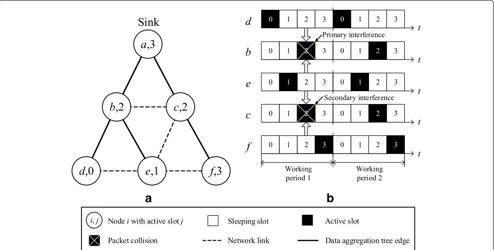
Figure1shows an example of the two types of interfer-ence that can occur in data aggregation scheduling, based on our assumption. A letter and a number in each node represent its node ID and active slot, respectively. Each working period is composed of four time slots, i.e., duty cycle 25%. A black slot represents active state, and a white slot represents sleep state. Data from all nodes is collected to the sink nodea. If nodesdandesend data to nodeb in the same working period, a collision, caused by primary interference, happens at nodeb. A secondary interference, resulting in a collision at nodec, occurs if nodeseandf send data to nodesb andcin the same working period, respectively.
3.2 Problem formulation
a
b
Fig. 1An example of collision in data aggregation scheduling in duty-cycled WSNs.aNetwork topology.bDuty-cycled schedule
its own data and data received from neighbors toward the sink node through a multi-hop path. A complete data aggregation function, such as COUNT, MIN, MAX, SUM, and AVERAGE, is deployed to ensure that every packet has the same size [2]. Anaggregation scheduleassigns a working period and a receiving node to every node, except the sink, for transmitting a data packet. The scheduled transmission must be collision-free while the maximum assigned working period is minimized.
In this paper, letG=(V,E)denote the communication graph of a duty-cycled WSN, whereVis the set of vertices, andEis the set of edges. We denote a sink node and the set of scheduled senders sending data in working period mbys∈VandSm, respectively. An aggregation schedule is defined as S = Dm=1Sm, whereDis theaggregation delayto the sink. The aggregation delay is determined by the largest value of scheduled working periodm, among all nodes in the WSN. The dc-MTAS problem is formally defined as:
Finding a data aggregation scheduleSwhich minimizes Ds.t.
(i) S=Dm=1Sm=V\ {s}.
(ii) Sm∩Sn= ∅,∀m=n.
(iii) Any pair of transmissions of senders in
Sm(1≤m≤D)are not conflicting.
(iv) All data are aggregated to the sinks in D working periods.
The dc-MTAS problem is an NP-hard problem [23].
4 Delay-aware data aggregation scheduling
We present details of our proposed data aggregation scheduling in this section. The scheme has two phases: the layered network structure construction phase and collision-free scheduling phase. The first phase, delay-aware tree construction (DTC), builds a CDS tree tak-ing the delay between nodes in a duty-cycled WSN into account and prepares a virtual backbone for efficient data aggregation in the network. The second phase, first-fit aggregation scheduling (FAS), conducts a fast collision-free data aggregation schedule based on the constructed backbone. Table1shows the notations used in this paper.
4.1 Delay-aware tree construction
As shown in Algorithm 1, DTC algorithm is composed of three steps. In step 1, it constructs a BFS tree rooted at sink nodes∈Vof a networkG=(V,E)(line 1). All nodes in the network are divided into layersL0,L1,. . ., andLlmax
according to the hop distance froms(line 2), wherelmaxis the largest layer in the BFS tree. LayerL0contains only the sink node. The sink is initially selected as a dominator and added to a dominating setDS(line 3). The algorithm exe-cutes multiple iterations of steps 2 and 3 from layer 1 to layerlmaxto construct a CDS tree rooted ats. To facilitate the delay-aware tree construction, DTC algorithm deter-mines thesleep delaybetween every pair of nodes(u,v)as follows:
d(u,v)=
a(v)−a(u), ifa(v) >a(u)
Table 1Notation
N(u) Set of neighbor nodes of nodeu
a(u) Active slot of nodeu
τ The number of time slots in a working period
Li Set of nodes in layeri
TCDS Connected dominating set tree
CD Set of candidate dominators
DS Set of dominators
P(u,v) The shortest path in terms of delay from nodesutov
d(u,v) Delay from nodesutov
d2d(u) The smallest delay from nodeuto upper dominator within 2-hop
p(u) Parent of nodeuinTCDS
Ox(u) Set of overhearing working periods of nodeu
Tx(u) Set of forbidden transmission working periods of nodeuto avoid collision
rx(u) The last receiving working period of nodeu
tx(u) Schedule for transmission of nodeu
Thed(u,v)shows the delay for which nodeuhas to wait to send data to nodev, at the active time slot of nodev. The sleep delay of a path is the accumulated sleep delays of all edges in the path.
LetLi be the set of nodes in layer i (1 ≤ i ≤ l). In step 2, nodes inLi, which are not adjacent with any domi-nator, become candidate dominators and are added to set CD(line 5). The shortest paths in terms of delay from a candidate dominator to all dominators within two-hop distance are established to identify the nearest dominator of the candidate (line 7). Such a dominator always exists in the upper layerj(0 ≤ j < i) because of the network connectivity. The shortest path from a candidate domi-nator to its nearest domidomi-nator, and the sleep delay of the path are recorded for further use (lines 8–9). LetP(u,v) denote the shortest path in terms of delay between candi-date dominatoruand its nearest dominatorv. The sleep delay ofP(u,v)isd2d(u) = d(u,w)+d(w,v), wherewis the intermediate node of the path.
DTC algorithm selects dominators among the candi-dates and then builds a CDS treeTCDSto connect all the dominators in step 3. Initially, the tree contains only sink nodes. In each layer, node u ∈ CDis selected to be a dominator if it has the smallest value ofd2d(u)among all nodes in the candidate dominator set. The selected dom-inator and all of its neighbors are removed from the set (lines 11–12). Nodeuand the intermediate nodewon the pathP(u,v)are added toTCDS (lines 13–14). Nodewis referred to as a connector and becomes the parent node p(u)of nodeuin the tree. It is worth noting that the near-est dominatorvof nodeuis already inTCDSand becomes
Algorithm 1:Delay-aware tree construction
Input :G=(V,E),s∈V
Output: A CDS treeTCDS=(VCDS,ECDS)
// Step 1: Construct layered structure
1 Construct a breadth first search tree rooted at sink
nodes
2 Divide all nodes inVinto layer setsL0,L1,. . ., and Llmaxaccording to hop distance froms
3 VCDS← {s},ECDS ← ∅,DS← {s} 4 fori←1to lmaxdo
// Step 2: Find the shortest path and update delay to dominator
5 CD←Li\ {u|u∈v∈DSN(v)} 6 foreachu∈CDdo
7 v←the nearest dominator in the upper layers
of nodeu
8 P(u,v)←the shortest path fromutov
9 d2d(u)←d(u,w)+d(w,v)// w is the intermediate node of the path P(u,v)
// Step 3: Construct delay-aware CDS tree
15 Update the layer sets andlmaxaccording to theTCDS
p(w). DTC algorithm iterates step 2 and step 3, layer-by-layer, until the layerlmax. It then updates the layer sets and lmaxsuch that every node is in the adjacent lower layer of its parent inTCDS(line 15). We refer to nodes that are not in the CDS tree as dominatees.
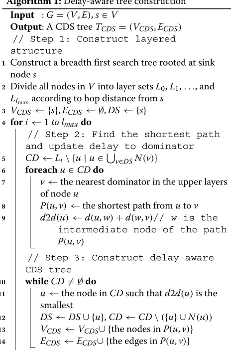
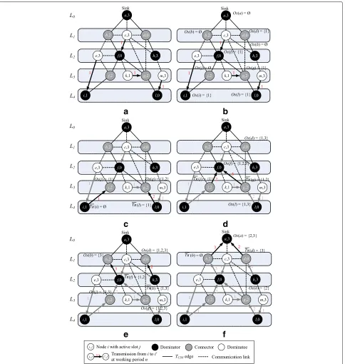
Figure2shows an example of DTC algorithm on a
net-work of 13 nodes with a duty cycle of 25% (τ = 4).
Nodes in the network are divided into layers as shown in Fig.2a. Initially, sink nodeais selected as a dominator and added to the tree. All nodes in layer 1 become domina-tees as they are adjacent toa. All nodes inL2= {e,f,g,h} become candidate dominators. The delays of all paths from a candidate dominator to nodea, the two-hop upper
dominator, are shown in Fig. 2b. The algorithm
a
b
c
d
e
f
Fig. 2An example of delay-aware tree construction.aStep 1: constructing layered structure.bStep 2 inL2: calculating delay from candidate dominator to upper dominators.cStep 2 inL2: finding the shortest path in terms of delay.dStep 3 inL2: adding dominators and connectors to the CDS tree.eStep 2 and step 3 inL3.fUpdating layer sets according toTCDS
a dominator. In Fig.2d, the dominatorsf andhare con-nected to the CDS tree by the two connectors ofbandd, respectively. Figure2eillustrates the process of DTC algo-rithm for nodes in layer 3. Finally, in Fig.2f, the layer sets are updated based on the CDS tree. The layers of nodes g, i, and lare increased to be bigger than those of their corresponding parents.
4.2 First-fit aggregation scheduling
Referring to the CDS tree TCDS of a WSN as an
aggregation backbone, the FAS scheme constructs a
delay-efficient schedule, gathering data from all nodes in the network to the sink. The scheduling scheme consists of two steps. It first collects data from all dominatees to nodes in the backbone and then collision-free aggre-gates the data from the backbone nodes to the sink in a bottom-up manner. It is worth noting that the backbone nodes include all dominators and connectors selected in DTC algorithm.
into two disjoint setsRandS, the set of nodes in the back-bone and the set of dominatees, respectively (line 1). Each dominatee inSis adjacent to at least one backbone node in R, i.e., its dominator. Starting from working period 1, the algorithm assigns a working period for each sending node inSso that its data packet can be delivered collision-free to a receiving node inR. The assigned working periods should be as small as possible to enable a minimum delay aggregation.
Algorithm 2:Dominatee scheduling
Input :G=(V,E),TCDS= {VCDS,ECDS},τ
Output: A transmitting scheduletx(u)for each node u∈V\VCDS
// Schedule |Ci| transmissions at
slot i of working period m
9 foreachu∈Cido
To ensure collision-free data collection, dominatee scheduling groups the receiving nodes into different sub-setsRi, where 0 ≤ i < τ, according to their active slots (lines 3–4). LetSidenote the subset of sending nodes adja-cent to nodes inRi (line 7). Algorithm 2 searches for a minimal subsetCi ⊂ Ri that can cover all nodes inSi (line 8). According to the property of the minimal cover set, each nodeu ∈ Cimust have at least one proprietary neighborv ∈ Si, which is only adjacent tou(line 10). If a receiving node has more than one proprietary neigh-bor, the algorithm randomly selects one of the neighbors as a sending node. We denote the transmitting schedule of nodev∈ Si bytx(v) = m,u(line 11), meaning that nodevis scheduled to send a data packet to nodeuat time
slota(u)=iof them-th working period. Obviously, there are|Ci|such pairs of neighboring nodes in each active slot i. The transmissions between the pairs of nodes can be
scheduled simultaneously in the same working periodm
without any collision.
After dominatee v is scheduled to transmit its data
packet, it is removed from the sending node setS (lines 11–12). Although only the corresponding receiving node u∈Ciis ensured to receive the packet in working period m (line 13), all nodes in N(v) ∩ Ri can overhear the transmission because they are active at the same time sloti. Algorithm 2 records the overheard working period for the neighbor nodes to prevent later transmissions from interfering (lines 14–15). The remaining domina-tees will be scheduled iteratively at the next active slots, and then the next working periods, until all dominatees are scheduled (line 16). It is worth noting that trans-missions at different active slots will not interfere with each other.
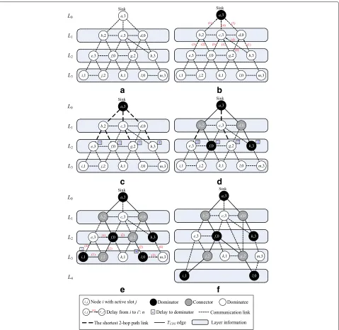
Figure3illustrates the dominatee scheduling algorithm on the same network as the example of DTC algorithm in Section4.1. Recall that a working period has four time slots, i.e.,τ = 4, in this example. According to the con-structedTCDS shown in Fig.3a, all nodes are separated into a sending setS= {c,e,k,m}and a receiving setR=
{a,b,d,f,h,j,g,i,l}, as in Fig.3b. The Algorithm 2 sched-ules transmissions from nodes inSto nodes inRat each active slot, iteratively. At active slot 0, only nodes inR0=
{d,f,i} can receive data packets from their neighbors in S0 = {c,e,k,m}. A minimal cover setC0 = {f,l} ⊂ R0is constructed to cover all nodes inS0. There are|C0| = 2 transmissions to receiving nodesf andlfrom their corre-sponding proprietary neighborscandmscheduled in the same working period, as in Fig.3c. In the same manner, the algorithm schedules transmissions from the remain-ing sendremain-ing nodeseandkto the receiving nodesiandg at active slots 1 and 2, as shown in Fig.3d,c, respectively. The dominatee data collection process completes, since all dominatees have been scheduled to transmit their data to nodes in theTCDS, as in Fig.3f.
a
b
c
d
e
f
Fig. 3An example of dominatee scheduling.aLayered network structure.bSeparating nodes into receiving and sending sets.cScheduling at active slot 0, working period 1.dScheduling at active slot 1, working period 1.eScheduling at active slot 2, working period 1.fTransmissions in the same working period
in the first step. A leaf node, which did not receive any data from dominatees, is ready at working period 1.
Note that all neighbors of node u active at the same
time slot with node p(u) can overhear a transmission
from u to the parent node. The transmission of u may
result in collisions at the neighbor nodes by interfering with other scheduled transmissions. To ensure collision-free data aggregation, the backbone scheduling algorithm collects all working periods in which such neighbors in TCDSof nodeuoverhear other scheduled transmissions. It refers to such working periods as forbidden working period ofuand stores them inTx(u)(lines 5–6). The algo-rithm prevents nodeufrom transmitting a packet in the working periods and searches for the minimum transmit-ting working period foru(lines 7–8). The last receiving working period of p(u) and overhearing working peri-ods of all neighbors active ata(p(u))inTCDS of nodeu
are updated for further collision avoidance. Algorithm 3 assigns a first-fit working period for each node in the tree in a bottom-up manner so that data from all nodes is aggregated at the sink node.
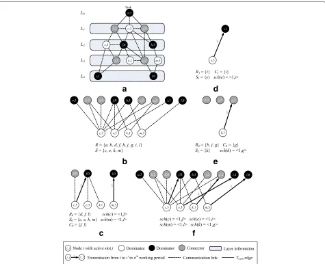
Figure4shows the process of the backbone scheduling algorithm on the same network as the example of DTC
algorithm in Section 4.1. According to the dominatee
data collection schedule in Fig. 3f, transmissions of
the dominatees are redrawn in Fig. 4a. The
overhear-ing workoverhear-ing periods caused by the transmissions are
updated for backbone nodes, as shown in Fig. 4b. The
Algorithm 3 starts from nodes in L4 = {i,l}, as shown
in Fig. 4c. Since the overhearing working period sets
of all neighbors of node i are empty, the forbidden set Tx(i) = ∅. As node i is active before its parentj in a working period, ican transmit a packet tojin the same
a
b
c
d
e
f
Fig. 4An example of delay-aware tree construction.aScheduling dominatees to nodes inTCDS.bOverhearing periods after dominatees scheduling. cScheduling for nodes inL4ofTCDS.dScheduling for nodes inL3ofTCDS.eScheduling for nodes inL2ofTCDS.fScheduling for nodes inL1ofTCDS
the other hand, nodeldelays its transmission to working period 2 because its parent nodeg is busy with a sched-uled transmission from dominateekin working period 1. The schedules of transmissions from nodes inL3,L2, and L1 are shown in Fig.4d–f, respectively. The data aggre-gation schedule in this example completes at working period 3.
5 Results and discussion
5.1 Theoretical analysis
5.1.1 Correctness
4 else m←rx(u)+1
// Collect the forbidden working
periods of node u
5 N←N(u)∩ {v|v∈VCDS, a(v)=a(p(u))} 6 Tx(u)←v∈NOx(v)
// Calculate first-fit working
period m for node u
7 whilem∈Tx(u)do m←m+1 8 tx(u)← m,p(u)
// Update receiving period and sets of overhearing working periods
9 rx(p(u))←m
10 foreachv∈Ndo 11 Ox(v)←Ox(v)∪ {m}
both primary and secondary interferences in its collision-free scheduling. We prove that the FAS scheme generates a collision-free aggregation schedule, as follows:
Theorem 1The FAS scheme provides a collision-free data aggregation scheduling.
ProofThe FAS scheme consists of two algorithms dom-inatee scheduling and backbone scheduling, which sched-ule transmissions from dominatee nodes and backbone nodes, i.e., dominators and connectors, respectively. The schedule of all dominatees is a collision-free schedule [23]. We only need to prove that there is no collision between any transmission of dominators and connec-tors. The fact is proven by contradiction. Assume that
there are two transmissions from nodes u and v
inter-fering with each other, and this results in a collision at
their common neighbor w. Without a loss of
general-ity, we assume that p(u) = w and the transmission
of u is scheduled before the one of v. When
schedul-ing node v, forbidden set Tx(v) contains the overhear-ing workoverhear-ing period of p(u) which is the transmitting
working period of node u. According to Algorithm 3,
the transmitting working period of v should not be
in Tx(v) and thus is different from the one of u. In
other words, the two transmissions from u and v are
time complexity is calculated in the worst case of each algorithm.
Theorem 2 The time complexity of SA scheme (LSC+WPS) is at most O(N2), where N is the number of nodes in a network andis the maximum node degree of the network.
Proof Initially, LSC algorithm takes at mostO(N2)time to divide the network graphGinto layers through a BFS tree [31]. Next, it takes at mostO(N)time to construct a MIS. Finally, the algorithm completes the layered net-work structure based on the CDS tree, by constructing connector sets with a layer update. The time complex-ity of this step is O(N). We combine all these steps and conclude that the time complexity of LSC is at most O(N2)+O(N)+O(N)=O(N2).
Based on the layered network structure of LSC, WPS algorithm schedules dominatees first and schedules dom-inators and later connectors in CDS layer-by-layer. To avoid collision, the scheduling process uses a sub-algorithm, which is the same as the Algorithm 2 of our proposed scheme. First, the sub-algorithm receives as input a sending set and a receiving set. The receiving set is separated by each active time slot i from 0 to τ − 1
(0 ≤ i ≤ τ − 1,O(N) time). Next, the sub-algorithm
conducts collision-free scheduling by selecting a minimal cover set of each sending set, which is covered by the classified receiving set. It takes at mostO(|Ri|)time to construct the minimal cover set in each active time sloti. Considering all the active time slots, the time complexity is((|R0| + |R1| +. . .+ |Rτ−2| + |Rτ−1|))=O(|R|)= O(N).
time complexity of SA (LSC+WPS) isO(N2)+O(N2)= O(N2).
Theorem 3The time complexity of our proposed scheme (DTC+FAS) is at most O(N2+N2log).
ProofThe first step of the DTC algorithm divides the network into layers, by constructing a BFS tree, taking O(N2). Next, DTC constructs a CDS tree, by repeating step 2 and step 3, from layer 1 to the last layer lmax of BFS tree. Step 2 constructs a set of candidate dominators CD, based on the nodes in each layer, and finds the short-est sleep delay path of the nodes inCD. Considering the nodes inCDof each layer, it takes at mostO(N)time for all layers. Finding the shortest delay path from each candi-date dominator to upper dominators takes at mostO(2) time. Therefore, the time complexity of step 2 isO(N2). Step 3 constructs a CDS tree with a set of dominators from the candidate dominators. It takesO(NlogN)time to sort theCDset for all layers. The algorithm uses the sortedCD to construct the CDS tree; thus, it has a time complexity ofO(NlogN+N). After that, DTC takes at mostO(N) time to update layers of parent and child nodes in the CDS tree. Finally, the time complexity of DTC is at most O(N2)+O(2N)+O(NlogN+N)=O(N2+2N). Next, in FAS scheme, scheduling the dominatees takes at most O(N2) time, similar to the sub-algorithm of WPS. Then, the process of updating a set of overhear-ing workoverhear-ing periods of dominators and connectors can be completed inO(N2)time. Therefore, the time com-plexity of the dominatee scheduling is at mostO(N2). In the conduction of an iterative schedule for domina-tors and connecdomina-tors in the CDS tree, it takes at most O(N) to collect nodes of a layer. To avoid collision, and to reduce the data aggregation delay, Algorithm 3 uses a set of forbidden transmission working periods and selects the first-fit transmission time for each node in the layer. In this process, constructing a set of forbid-den transmission working periods of each node takes at most O(N2log) time and the first-fit scheduling takes at most O(N2) time. Lastly, the time complex-ity for updating the sets of overhearing working peri-ods for neighbors of the scheduled node is O(N2). Therefore, the backbone scheduling has a time
com-plexity of O(2Nlog + N2 + N2) = O(N2 +
2Nlog). Accordingly, the time complexity of FAS
is O(N2 + 2Nlog). From the above analyses, we
combine the time complexity of DTC and FAS. The time complexity of our proposed scheme (DTC+FAS) is O(N2 + 2N) + O(N2 + 2Nlog) = O(N2 + 2Nlog).
The time complexity analysis results show that SA has a lower complexity than our proposed scheme. The
difference becomes negligible when theis small in the real WSN deployment environments.
5.2 Simulation evaluation
In this section, we evaluate the performance of our pro-posed scheme, through in-depth simulation in various scenarios. The simulation environment is as follows. First, we use a unit disk graph (UDG) for simulation and ran-domly deploy nodes in a region of 200m×200m. These nodes have the same transmission range and use an iden-tical channel. A sink is located at a top-left corner. We vary the duty cycle of the network, via the number of time slots
τin a working period. The duty cycles used in our simula-tion are 50, 33.33, 25, 20, 12.5, 10, 6.67, 5, 3.33, 2, 1.25, and 1%, corresponding toτ = 2, 3, 4, 5, 8, 10, 15, 20, 30, 50, 80, and 100, respectively. Here, an active time slot of each node is randomly and independently determined between time slots 0 andτ − 1 [27]. The sink knows the active time slots of all the nodes, with the network information. Our proposed scheme performs in a centralized manner at the sink. The simulation for each setting is conducted 100 times, and the average value is plotted.
We use the data aggregation time as an evaluation met-ric. It is defined as the number of working periods for all data aggregated at the sink, in duty-cycled WSNs. We
implement SA (LSC + WPS) [23], to compare its
per-formances with our proposed scheme (DTC + FAS), in terms of data aggregation time. Moreover, for detailed analysis between SA and our proposed scheme, we also compare with the two schemes of (LSC + FAS) and (DTC + WPS). The rest of this section presents the results of the performance analysis, according to different scenarios.
5.2.1 Impact of node density
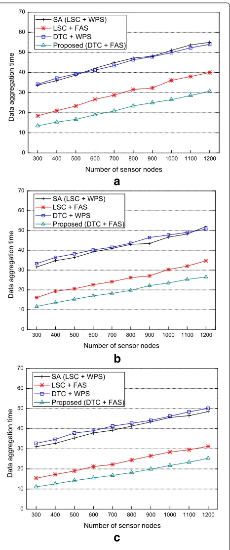
Figure 5 illustrates the data aggregation time of each
scheme, when the number of nodes increases from 300 to 1200 nodes. In this scenario, the transmission range of a node is fixed to 30m, and the duty cycle is set to 20,
10, and 5% (τ = 5, 10, and 20). The simulation result
a
b
c
Fig. 5Data aggregation time with different number of nodes. aτ=5 .bτ=10 .cτ=20 (5% duty cycle)
CDS tree. On the other hand, WPS generates an addi-tional delay, due to collision avoidance. It uses the largest working period, which is scheduled in the lower layer,
However, WPS in SA schedules each node, regardless of the CDS tree constructed by DTC. In other words, it can-not utilize the shortest path, in terms of delay. Therefore, SA (LSC + WPS) and DTC + WPS have similar results. On the other hand, FAS effectively utilizes the advantage of DTC, by scheduling the nodes of each layer, using the first-fit method. In particular, in the shortest path, the sending node has a better chance of directly transmit-ting to the receiving node in its last receiving working period. In Fig.5a–c, the proposed scheme (DTC + FAS) based on DTC improves data aggregation time perfor-mance by up to 28, 29, and 28%, compared to LSC + FAS based on LSC.
5.2.2 Impact of duty cycle
In the second scenario, we compare and analyze the data aggregation time of each scheme in different duty-cycled environments, unlike the first scenario. The transmission range of nodes is fixed to 30 m, and the number of nodes is fixed to 1000 nodes. Here, the duty cycle reduces from 50 to 1%, i.e.,τ =2, 3, 4, 5, 8, 10, 15, 20, 30, 50, 80, and 100. In this scenario, we set the number of nodes to 200, 600, and 1000 for simulation.
Figure6a–crepresents the data aggregation time of each scheme, with different duty cycles. The simulation result shows that the more the duty cycle decreases, the more the data aggregation time is reduced. Here, each scheme does not show a significant difference, since the duty cycle is 10% (τ = 10). The reason is that the number of nodes receiving data is fixed, even though the chances of send-ing data without collision is increased (i.e., the saturation state). Meanwhile, if we get the data aggregation time in terms of the number of time slots in this scenario, more delay is incurred, due to an inverse relationship between the working period and the time slot of the data aggrega-tion time. Our proposed scheme (DTC+FAS) in Fig.6a–c
also outperforms SA (LSC+WPS) under a different duty cycles scenario. Overall, the data aggregation time of our proposed scheme (DTC+FAS) is up to 67, 60, and 55% shorter than that of SA (LSC+WPS).
5.2.3 Impact of transmission range
a
b
c
Fig. 6Data aggregation time with different duty cycles.aNumber of nodes = 200.bNumber of nodes = 600.cNumber of nodes = 1000
increase the delay for data aggregation. In the third sce-nario, we evaluate the data aggregation time of each scheme, according to the different transmission range of
each node. The number of nodes is fixed at 600 and the duty cycle is 10
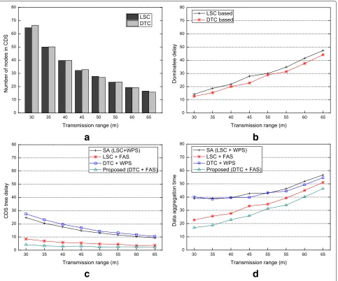
Figure7ashows that the number of dominators and con-nectors is reduced, when the transmission range increases at the first phase of each scheme, i.e., the number of nodes in CDS is reduced. Otherwise, the number of domina-tees is increased. Thus, the delay of transmissions from dominatees to nodes in CDS increases, as the transmis-sion range increases, as in Fig.7b. WPS and FAS at the second phase of each scheme use the same method for dominatee scheduling (Algorithm 3). However, they have different features when they schedule nodes in the CDS tree layer-by-layer. Figure7cshows the time duration for data aggregation to a sink based on the CDS tree regard-ing WPS and FAS. The result is the calculated delay, when each scheduling algorithm schedules dominators and connectors layer-by-layer. The schemes using WPS have lower performance than those using FAS, due to the additional delay of updating layer-by-layer, like other scenarios.
Figure 7d shows the data aggregation time of each
scheme, when the transmission range increases. The result is the same as combining Fig. 7b, c; the data aggregation time increases when the transmission range increases. In particular, FAS incurs the same delay as WPS in dominatee scheduling, but it generally outper-forms WPS. The reason is that FAS uses a first-fit method for each node in the CDS tree aggregation scheduling. The method schedules nodes to send data at the fastest available transmission time, if no collision occurs. In this scenario, our proposed scheme (DTC + FAS) can improve data aggregation time compared with SA (LSC + WPS) by up to 72%.
6 Conclusions
In this paper, we proposed a scheme for collision-free data aggregation scheduling in duty-cycled WSNs, which significantly reduces the data aggregation delay. Our pro-posed scheme, based on a centralized approach, consists of the DTC algorithm and FAS algorithm for efficient data aggregation. Our proposed scheme reduces data aggre-gation time to the sink, through delay-aware scheduling in duty-cycled WSNs. We proved the correctness of the collision-free algorithm of our proposed scheme by con-tradiction. In addition, we analyzed the time complexity of our proposed scheme. The analyses showed that our proposed scheme has similar or higher complexity than SA. However, the simulation results show that our pro-posed scheme significantly reduces data aggregation time, compared to SA.
a
b
c
d
Fig. 7Performance evaluation with different transmission ranges.aNumber of nodes in CDS.bDominatee aggregation delay.cCDS tree aggregation delay.dData aggregation time
efficient data aggregation scheduling. Moreover, we will continue this work, considering not only a protocol inter-ference model, but also a physical interinter-ference model [32], which is appropriate for a real propagation environment.
Abbreviations
BFS: Breadth first search; CDS: Connected dominating set; dc-MTAS: Minimum time aggregation scheduling in duty-cycled WSNs; DTC: Delay-aware tree construction; FAS: First-fit aggregation scheduling; LSC: Layered structure construction; MIS: Maximal independent set; MTAS: Minimum time aggregation scheduling; SA: Scheduling algorithm; SDA: Shortest data aggregation; SPT: Shortest path tree; WPS: Working period scheduling; WSN: Wireless sensor network
Acknowledgements
This research was supported in part by the Korean government, under the G-ITRC support program (IITP-2016-R6812-16-0001) supervised by the IITP, Priority Research Centers Program (NRF-2010-0020210), Autonomous Network Control and Management (B0101-15-1366), and Basic Science Research Program (NRF-2016R1D1A1B03934660) through NRF, respectively.
Authors’ contributions
This paper has been conducted by DTL under the supervision of HC. TL contributed to the performance evaluation of the proposed algorithms presented in the paper. All authors read and approved the final manuscript.
Competing interests
The authors declare that they have no competing interests.
Publisher’s Note
Springer Nature remains neutral with regard to jurisdictional claims in published maps and institutional affiliations.
Received: 24 July 2017 Accepted: 18 April 2018
References
1. IF Akyildiz, W Su, Y Sankarasubramaniam, E Cayirci, A survey on sensor networks. IEEE Commun. Mag.40(8), 102–114 (2002).https://doi.org/10. 1109/MCOM.2002.1024422
aggregate queries over ad-hoc wireless sensor networks, (2002), pp. 49–58.https://doi.org/10.1109/MCSA.2002.1017485
3. R Cristescu, B Beferull-Lozano, M Vetterli, inIEEE INFOCOM 2004, vol. 4. On network correlated data gathering, (2004), pp. 2571–25824.https:// doi.org/10.1109/INFCOM.2004.1354677
4. YP Chen, AL Liestman, J Liu, A hierarchical energy-efficient framework for data aggregation in wireless sensor networks. IEEE Trans. Veh. Technol.
55(3), 789–796 (2006).https://doi.org/10.1109/TVT.2006.873841 5. S Manishankar, PR Ranjitha, TM Kumar, in2017 International Conference on
Communication and Signal Processing (ICCSP). Energy efficient data aggregation in sensor network using multiple sink data node, (2017), pp. 0448–0452.https://doi.org/10.1109/ICCSP.2017.8286397
6. S Wan, Y Zhang, J Chen, On the construction of data aggregation tree with maximizing lifetime in large-scale wireless sensor networks. IEEE Sensors J.16(20), 7433–7440 (2016).https://doi.org/10.1109/JSEN.2016.2581491 7. HC Lin, WY Chen, An approximation algorithm for the maximum-lifetime
data aggregation tree problem in wireless sensor networks. IEEE Trans. Wirel. Commun.16(6), 3787–3798 (2017).https://doi.org/10.1109/TWC. 2017.2688442
8. B Alinia, MH Hajiesmaili, A Khonsari, N Crespi, Maximum-quality tree construction for deadline-constrained aggregation in wsns. IEEE Sensors J.17(12), 3930–3943 (2017).https://doi.org/10.1109/JSEN.2017.2701552 9. Y Gao, X Li, J Li, Y Gao, Construction of optimal trees for maximizing
aggregation information in deadline- and energy- constrained unreliable wireless sensor networks. IEEE Access.PP(99), 1–1 (2018).https://doi.org/ 10.1109/ACCESS.2017.2788877
10. X Chen, X Hu, J Zhu, inProceedings of the First International Conference on Mobile Adhoc and Sensor Networks (MSN’05). Minimum data aggregation time problem in wireless sensor networks (Springer, Berlin, 2005), pp. 133–142.https://doi.org/:10.1007/11599463_14
11. SCH Huang, PJ Wan, CT Vu, Y Li, F Yao, inIEEE INFOCOM 2007 - 26th IEEE International Conference on Computer Communications. Nearly constant approximation for data aggregation scheduling in wireless sensor networks, (2007), pp. 366–372.https://doi.org/10.1109/INFCOM.2007.50 12. X Xu, XY Li, X Mao, S Tang, S Wang, A delay-efficient algorithm for data
aggregation in multihop wireless sensor networks. IEEE Trans. Parallel Distrib. Syst.22(1), 163–175 (2011).https://doi.org/10.1109/TPDS.2010.80 13. G Anastasi, M Conti, MD Francesco, A Passarella, Energy conservation in
wireless sensor networks: A survey. Ad Hoc Netw.7(3), 537–568 (2009). https://doi.org/10.1016/j.adhoc.2008.06.003
14. G Lu, N Sadagopan, B Krishnamachari, A Goel, inProceedings IEEE 24th Annual Joint Conference of the IEEE Computer and Communications Societies, vol. 4. Delay efficient sleep scheduling in wireless sensor networks, (2005), pp. 2470–24814.https://doi.org/10.1109/INFCOM.2005.1498532 15. Y Gu, T He, Dynamic switching-based data forwarding for low-duty-cycle
wireless sensor networks. IEEE Trans. Mob. Comput.10(12), 1741–1754 (2011).https://doi.org/10.1109/TMC.2010.266
16. X Jiao, W Lou, J Ma, J Cao, X Wang, X Zhou, Minimum latency broadcast scheduling in duty-cycled multihop wireless networks. IEEE Trans. Parallel Distrib. Syst.23(1), 110–117 (2012).https://doi.org/10.1109/TPDS.2011.106 17. F Wang, J Liu, On reliable broadcast in low duty-cycle wireless sensor
networks. IEEE Trans. Mob. Comput.11(5), 767–779 (2012).https://doi. org/10.1109/TMC.2011.94
18. D-T Le, T Le-Duc, VV Zalyubovskiy, DS Kim, H Choo, LABS: Latency aware broadcast scheduling in uncoordinated duty-cycled wireless sensor networks. J. Parallel Distrib. Comput.74(11), 3141–3152 (2014).https:// doi.org/10.1016/j.jpdc.2014.07.011
19. T Le-Duc, D-T Le, VV Zalyubovskiy, DS Kim, H Choo, Level-based approach for minimum-transmission broadcast in duty-cycled wireless sensor networks. Pervasive Mob. Comput.27(C), 116–132 (2016).https://doi.org/ 10.1016/j.pmcj.2015.10.002
20. T Le-Duc, D-T Le, VV Zalyubovskiy, DS Kim, H Choo, Towards broadcast redundancy minimization in duty-cycled wireless sensor networks. Int. J. Commun. Syst. (2016).https://doi.org/10.1002/dac.3108
21. TD Nguyen, J Choe, T Le-Duc, D-T Le, VV Zalyubovskiy, H Choo, Delay-sensitive flooding based on expected path quality in low duty-cycled wireless sensor networks. Int. J. Distrib. Sens. Netw.12(8) (2016).https://doi.org/10.1177/1550147716664254
22. D-T Le, T Le-Duc, VV Zalyubovskiy, DS Kim, H Choo, Collision-tolerant broadcast scheduling in duty-cycled wireless sensor networks. J. Parallel Distrib. Comput.100, 42–56 (2017).https://doi.org/10.1016/j.jpdc.2016. 10.006
23. B Yu, J-Z Li, Minimum-time aggregation scheduling in duty-cycled wireless sensor networks. J. Comput. Sci. Technol.26(6), 962–970 (2011). https://doi.org/10.1007/s11390-011-1193-9
24. G Lu, B Krishnamachari, CS Raghavendra, in18th International Parallel and Distributed Processing Symposium, 2004. Proceedings. An adaptive energy-efficient and low-latency mac for data gathering in wireless sensor networks, (2004), pp. 224–231.https://doi.org/10.1109/IPDPS. 2004.1303264
25. Y Gu, T He, M Lin, J Xu, in2009 30th IEEE Real-Time Systems Symposium. Spatiotemporal delay control for low-duty-cycle sensor networks, (2009), pp. 127–137.https://doi.org/10.1109/RTSS.2009.12
26. T Lee, DS Kim, H Choo, M Kim, in2013 IEEE 9th International Conference on Mobile Ad-hoc and Sensor Networks. A delay-aware scheduling for data aggregation in duty-cycled wireless sensor networks, (2013), pp. 254–261. https://doi.org/10.1109/MSN.2013.69
27. O Dousse, P Mannersalo, P Thiran, inProceedings of the 5th ACM International Symposium on Mobile Ad Hoc Networking and Computing. MobiHoc ’04. Latency of wireless sensor networks with uncoordinated power saving mechanisms (ACM, New York, 2004), pp. 109–120.https:// doi.org/10.1145/989459.989474.http://doi.acm.org/10.1145/989459. 989474
28. M Maróti, B Kusy, G Simon, A Lédeczi, in2nd International Conference on Embedded Networked Sensor Systems. SenSys ’04. The flooding time synchronization protocol (ACM, New York, 2004), pp. 39–49.https://doi. org/10.1145/1031495.1031501.http://doi.acm.org/10.1145/1031495. 1031501
29. S Yoon, C Veerarittiphan, ML Sichitiu, Tiny-sync: Tight time
synchronization for wireless sensor networks. ACM Trans. Sens. Netw.3(2) (2007).https://doi.org/10.1145/1240226.1240228
30. P Gupta, PR Kumar, The capacity of wireless networks. IEEE Trans. Inf. Theory.46(2), 388–404 (2000).https://doi.org/10.1109/18.825799 31. TH Cormen, CE Leiserson, RL Rivest, C Stein,Introduction to algorithms, 3rd
edn. (The MIT Press, Cambridge MA 02142-1209, 2009)