R E S E A R C H
Open Access
A variational multiscale method for steady
natural convection problem based on
two-grid discretization
Xuesi Ma
1,2*, ZhenZhen Tao
2and Tong Zhang
2,3*Correspondence:
maxuesi@hpu.edu.cn
1Center for Intelligence Science and
Technology, School of Computer Science, Beijing University of Posts and Telecommunications, Beijing, 100876, P.R. China
2School of Mathematics &
Information Science, Henan Polytechnic University, Jiaozuo, 454003, P.R. China
Full list of author information is available at the end of the article
Abstract
In this paper, we propose and analyze a two-grid variational multiscale method for the steady natural convection problem based on two local Gauss integrations technique. This method possesses the best algorithmic characteristics of both variational multiscale method and two-grid discretization. The main idea is to first solve the nonlinear steady natural convection problem on the coarse grid, then to use the coarse grid solution to fix the nonlinear terms, and to solve a linear problem on the fine grid. Stability and optimal error estimates of the discrete solutions in both one-grid and two-grid variational multiscale formulations are established. Finally, some numerical examples are presented to verify the method’s promise and testify the theoretical predictions.
Keywords: natural convection problem; two-grid discretization; Oseen iteration; variational multiscale method; error estimates
1 Introduction
The natural convection phenomenon is present in many real situations such as room ven-tilation, double glass window design,etc.More importantly, it is behind the oceanic and atmospheric dynamics. Let⊂Rd (d= or ) be a regular bounded open domain, we
consider the following steady natural convection problem:
⎧ ⎪ ⎪ ⎪ ⎪ ⎪ ⎪ ⎨ ⎪ ⎪ ⎪ ⎪ ⎪ ⎪ ⎩
–Pru+ (u· ∇)u+∇p=Pr RaζT+γ, ζ=e/|e|, in,
∇ ·u= , in,
u= , on∂,
–∇ ·(k∇T) + (u· ∇)T=γ, in,
T= , onT, ∂∂Tn = , onB,
(.)
whereis a bounded convex polyhedral domain, the unknown functions are the veloc-ityu, the pressurep, and the temperatureT.eis a unit vector in the direction of gravi-tational acceleration,γ andγare known functions.nis the outward unit normal to,
andT=∂\BwhereBis a regular open subset of∂.Pr,Ra, andk> denote Prandtl
number, Rayleigh number, and thermal conductivity parameter, respectively.
The natural convection problem (.) is an important system with dissipative nonlinear terms in atmospheric dynamics. This system not only contains the velocity and pressure,
but also includes the temperature field, finding the numerical solution of problem (.) be-comes a difficult task. For the research of the natural convection problem (.), there have enormous works been devoted to the development of efficient schemes ([–] and the ref-erences therein). For example, [, ] developed the mixed finite element method (FEM) for problem (.). Cibik and Kaya [] constructed a projection-based stabilization finite ele-ment method. Galvinet al.[] studied problem (.) with poor mass conservation in mixed finite element algorithm for flow problems of large rotation-free forcing in the momen-tum equations. Zhanget al.[] developed the decoupled two-grid method. For the time-dependent case, Benítez and Bermúdez [] considered a second order Lagrange-Galerkin method. Boland and Layton [] presented stability and error estimates for the Galerkin fi-nite element spatial semi-discretization case. Manzari [] used standard Galerkin FEM in spatial discretization and an explicit multistage Runge-Kutta scheme in the time domain for convection heat transfer problem.
It is well known that the small viscous problem is a challenge subject due to the sin-gularity of the numerical solutions. As a result, much attention has been appealed to the recent years. There are several numerical schemes have been developed for the simula-tion of small viscous flows, such as the decoupled method [], the variasimula-tional multiscale method [–], the defect-correction method [, ] and so on. Among them, the vari-ational multiscale method is a popular numerical technique. This method is on the base of the decomposition of the flow scales and definition of the large scales that is projected into appropriate subspaces. In this work, we propose a new variational multiscale method by defining the stabilization terms via two local Gauss integrations based on projection operators. A significant feature of this new variational multiscale method is that the stabi-lization terms are defined by the difference between a consistent and an under-integrated matrix only involving the velocity gradient (and temperature gradient), rather than the projection operator as used in the common variational multiscale method. This new vari-ational multiscale method does not need to introduce extra variables and can keep good accuracy. Zhanget al.have made some numerical examples in [] to verify the efficiency of this new variational multiscale method for problem (.), Shang [] has presented an error analysis of two level subgrid stabilized Oseen iterative method for time-dependent Navier-Stokes equations. The main contribution of this work can be listed as follows. () The theoretical analysis of new variational multiscale method based on two local Gauss integrations for steady natural convection problem is provided. () A two-grid variational multiscale Oseen iterative scheme for the steady natural convection problem is developed, the corresponding error estimates are presented. Therefore, our work can be considered as an extension and supplement of the existing results [, , ].
2 Preliminaries
2.1 Mathematical setting and basic results
The function spaces for the velocityu, the pressurep, and the temperatureTare defined, respectively, by
X=H()d=v∈H()d:v= on∂,
M=L() =p∈L() : (p, )=
,
W=S∈H() :S= onB
,
V=H,div () ={v∈X:∇ ·v= in},
where the spacesL()m,m= , , are equipped with the standardL-scalar product (·,·) andL-norm · ,Hj() denotes the standard Sobolev space with norm · j. The space Xis endowed with the usual scalar product (∇u,∇v) and the norm∇u.
The weak form of (.) reads as follows: Find (u,p,T)∈X×M×Wsuch that
Pra(u,v) +c(u,u,v) +b(v,p) –b(u,q) =Pr Ra(Tζ,v) + (γ,v),
ka¯(T,S) +c¯(u,T,S) = (γ,S),
(.)
for all (v,q,S)∈X×M×W, where
a(u,v) = (∇u,∇v), a¯(T,S) = (∇T,∇S), b(v,q) = –(∇ ·v,q),
c(u,v,w) = (u· ∇)v,w+
(∇ ·u)v,w
=
(u· ∇)v,w
–
(u· ∇)w,v
,
¯
c(u,T,S) = (u· ∇)T,S+
(∇ ·u)T,S
=
(u· ∇)T,S
–
(u· ∇)S,T
.
The following lemma and theorem provide some important results for bilinear terms
a(·,·),a¯(·,·) and the existence and uniqueness of solutions for problem (.).
Lemma .(see []) For all u,v,w∈X and S,T∈W,the following estimates hold.
a(u,v)≤ ∇u∇v, a(u,u)≥ ∇u,
a¯(T,S)≤ ∇T∇S, a¯(T,T)≥ ∇T,
c(u,v,w)≤N∇u∇v∇w, c(u,v,v)= ,
c(u,T,S)≤N∇u∇T∇S, c(u,T,T)= ,
where N=sup=u,v,w∈X∇u|c∇(u,vv,w)∇| w and N=sup=u∈X,=θ,ψ∈W
|c(u,θ,ψ)|
∇u∇θ∇ψ.
Theorem .(see []) Under the condition
Raγ–+
Pr–
k–+PrN k–
γ–≤
Pr k–+PrN
k–
, (.)
problem(.)admits a unique solution(u,T)and satisfies
2.2 The finite element spaces
To introduce the finite element discretization of (.), we assume Tμ() ={K} (here μ=H,hwithH h) to be a shape-regular triangulation ofinto triangles or quadri-laterals (ifd= ), or tetrahedrons or hexahedrons (ifd= ) with mesh size <μ< . The fine meshTh() is found by a mesh refinement process of the coarse mesh. It is of worth to mention that it is not necessary for our method, nor needed for the results of our con-vergence theorems to hold. However, we assume the coarse and fine grids nested since it will simplify our analysis substantially. LetXμ⊂X,Mμ⊂M,Wμ⊂W be three finite element spaces associated withTμ() and satisfying the following assumptions.
(A)Approximation. For each (u,p,T)∈Hk+()d×Hk()×Hk+(), there exists an
approximation (π
μu,ρμp,πμT) such that
∇ u–πμu≤cμsu+s, p–ρμp≤cusps, (.) ∇ T–πμT≤cμsT+s, ≤s≤k, (.)
here and below, the letterscandCdenote the general positive constants dependent at most on the coefficients of the equations and the domain, but independent of the mesh size and the iterative timesm, furthermore, they are different at their different occurrences.
(A)inf-supcondition. For the finite element spacesXμandMμ, there exists a constant β> such that
βqμ≤ sup
vμ∈Xμ,vμ=
(∇ ·vμ,qμ)
∇vμ
, ∀qμ∈Mμ. (.)
It is noted that many mixed finite element pairs such as the Taylor-Hood element, the MINI element, and theP-Pelement satisfy the above assumptions (A) and (A).
Set
Vμ=
vμ∈Xμ: (∇ ·vμ,qμ) = ,∀qμ∈Mμ
.
It is well known that (see [])
inf vμ∈Vμ
∇(v–vμ)≤C
+ β
inf vμ∈Xμ
∇(v–vμ), ∀v∈V. (.)
Under the above assumptions, the mixed finite element approximation of (.) reads: Find a pair (uμ,pμ,Tμ)∈Xμ×Mμ×Wμsuch that for all (vμ,qμ,Sμ)
Pra(uμ,vμ) +c(uμ,uμ,vμ) +b(vμ,pμ) –b(uμ,qμ) =Pr Ra(Tμζ,vμ) + (γ,vμ),
ka¯(Tμ,Sμ) +c¯(uμ,Tμ,Sμ) = (γ,Sμ).
(.)
The following theorem establishes the existence and uniqueness of the numerical solu-tions for problem (.) and provides the optimalL-norm error estimates.
Theorem .(see []) Under the assumptions of(A), (A),and some assumptions as re-gards the k,Pr,Ra,γ,γ,problem(.)possesses a unique solution(uμ,pμ,Tμ)and satisfies
3 The variational multiscale method based on two local Gauss integrations
In this section, we shall first formulate the variational multiscale method, and then develop the numerical scheme for the considered problem (.).
3.1 The variational multiscale method
Our variational multiscale method is based on two elliptic projection operators,
μ:X→R={v∈H()d:v|K∈(P)d,∀K∈Eμ()},
μ:W→R={S∈H() :S|K∈P,∀K∈Eμ()},
which can be defined as follows (see []):
∇μu,∇v= (∇u,∇v), ∀u∈X,v∈R,
∇μT,∇S= (∇T,∇S), ∀T∈W,S∈R,
and have the following properties:
∇μu≤ ∇u, ∀u∈X, ∇μT≤ ∇T, ∀T∈W, (.)
whereRandRare two spaces of polynomials of degree less than or equal to one.
Based on projectionsμandμ, we define the following stabilization terms:
G(u,v) =α ∇ I–μ
u,∇ I–μv, ∀u,v∈X, (.)
G(T,S) =α ∇ I–μ
T,∇ I–μS, ∀T,S∈W, (.) whereα,α> are two user-defined stabilization parameters, typically chosen asα=
α=O(μ)s(heres> is a constant related to the finite elements used for the discretization
of the considered problem).
Thanks to (.) and (.), the finite element variational multiscale method for problem (.) reads as follows: Find (uμ,pμ,Tμ)∈Xμ×Mμ×Wμsuch that
⎧ ⎪ ⎨ ⎪ ⎩
Pra(uμ,vμ) +c(uμ,uμ,vμ) +b(vμ,pμ) –b(uμ,qμ) +G(uμ,vμ) =Pr Ra(Tμζ,vμ) + (γ,vμ),
ka¯(Tμ,Sμ) +¯c(uμ,Tμ,Sμ) +G(Tμ,Sμ) = (γ,Sμ),
(.)
for all (vμ,qμ,Sμ)∈Xμ×Mμ×Wμ.
3.2 Stability and convergence of scheme (3.4)
The system (.) is nonlinear; it needs to be linearized in computations. A popular lin-earization process is the one based on the Newton iterative method. However, it is well known that the Newton iterative method is sensitive to the initial guess for the nonlin-ear iterations,i.e., to guarantee the convergence of the Newton iterations, the initial guess should be close enough to the solution (uμ,Tμ). Here we use the Oseen iterative method to solve (.).
From the definitions (.) and (.) of the projection operatorsμ,μ, we have
G(u,v) =α ∇ I–μ
u,∇ I–μv
=α(∇u,∇v) –α ∇μu,∇v
G(T,S) =α ∇ I–μ
T,∇ I–μS
=α(∇T,∇S) –α ∇μT,∇S
, ∀T,S∈W. (.)
By applying the Oseen iterative method to the nonlinear problem (.) and thanks to (.) and (.), we develop the variational multiscale Oseen iterative scheme for the natural convection problem: Find an iterative solution (unμ,pnμ,Tμn)∈Xμ×Mμ×Wμsuch that
⎧ ⎪ ⎨ ⎪ ⎩
(Pr+α)a(unμ,vμ) +c(unμ–,uμn,vμ) +b(vμ,pnμ) –b(unμ,qμ) =Pr Ra(Tn
μζ,vμ) + (γ,vμ) +α(∇μunμ–,∇vμ),
(k+α)a¯(Tμn,Sμ) +¯c(unμ–,Tμn,Sμ) = (γ,Sμ) +α(∇μTμn–,∇Sμ),
(.)
for all (vμ,qμ,Sμ)∈Xμ×Mμ×Wμ,n= , , . . . , withuμ= ,Tμ= .
Throughout this paper, we assume thatμis small enough such that the iterative scheme (.) is convergent. In order to keep notation brief, we define
A=Pr–γ–+Rak–γ–, B=k–γ–.
Theorem . The iterative solution(un
μ,Tμn)defined by(.)satisfies
∇unμ≤A, ∇Tμn≤B, ∀n≥. (.)
Proof LetSμ=Tμnin the second equation of (.), we have
(k+α)a¯ Tμn,Tμn
= γ,Tμn
+α ∇μTμn–,∇Tμn
.
We use the Cauchy-Schwarz inequality and (.) to obtain
(k+α)∇Tμn≤ γ–+α∇
μT
n–
μ ≤ γ–+α∇T
n–
μ .
Whenn= , we get
(k+α)∇Tμ≤ γ– ⇒ ∇T
μ≤
k+α
γ–≤k–γ–,
which shows that the second inequality of (.) holds forn= . We now assume it holds forn=Jand prove it holds forn=J+ ,
(k+α)∇TμJ+≤ γ–+α∇TμJ≤k–(k+α)γ–.
As a consequence one finds
∇TμJ+≤k –γ
–. (.)
Takingvμ=unμandqμ=pnμin the first equation of (.), and using (.), we obtain
(Pr+α)∇unμ≤ γ–+α∇
μunμ–+Pr RaT
n
μ–
Due to the facts thatα> anduμ= , we know that (.) holds forn= . Assume that
which with (.) completes the proof.
Theorem . Assume that (u,T)is the nonsingular solution to the natural convection
problem(.),αandαtend to zero asμtends to zero.Under the condition of
Remark . As the velocityuand temperatureT are coupled in system (.), the error
estimation forT–Tn
Proof Setting (en
μ,ηnμ,φμn) = (u–uμn,p–pnμ,T–Tμn) and subtracting (.) from (.), we obtain the following error equations for the variational multiscale Oseen iterative scheme:
⎧
In the same way, we have
¯
From the second equation of (.), one finds
(k+α) ∇εnμ,∇Sμ
Thanks to Theorem ., (.) and Theorem . we derive that
(k+α)∇εnμ≤(k+α+NA)∇ρ+NB∇e
n
μ
With the help of the triangle inequality one finds
Making use of Theorem . and Theorem ., we obtain
(Pr+α)∇ξμn≤(Pr+α+ NA)∇ρ+NA∇ unμ–unμ– +Pr Ra∇φμn+ αA+NA∇ξμn+
√
dp–λμ. (.)
To complete the proof, the bound (.) is inserted into the one of (.), this gives
thus
Under the condition of (.) we find that
Now, we present the convergence ofp–pn
μ. Lettingλμbe an approximation ofpinMμ
Corollary . Under the condition of Theorem.,the solution(un
μ,pnμ,Tμn)∈Xμ×Mμ×
Wμdefined by(.)satisfies
∇ u–unμ+p–p
n
μ+∇ T–T
n
μ
≤cμs+Cα+Cα+C∇ unμ–u
n–
μ .
Remark . Corollary . shows that to ensure a good approximation, the variational
multiscale Oseen iterations should converge sufficiently. Moreover, the estimator suggests the choice of the stabilization parametersα=O(μs) andα=O(μs) which ensure optimal
convergence.
4 Two-grid variational multiscale method
Combining two-grid discretization strategy with the variational multiscale Oseen iterative method presented in the previous section, we develop the two-grid variational multiscale Oseen iterative method as follows.
Step. Find a coarse grid iterative solution (umH,pmH,THm)∈XH×MH×WHsuch that
⎧ ⎪ ⎨ ⎪ ⎩
(Pr+α)a(umH,vH) +c(umH–,uHm,vH) +b(vH,pmH) –b(umH,qH)
=Pr Ra(THmζ,vH) + (γ,vH) +α(∇HumH–,∇vH),
(k+α)a¯(THm,SH) +¯c(umH–,THm,SH) = (γ,SH) +α(∇HTHm–,∇SH),
for all (vH,qH,SH)∈XH×MH×WH,n= , , . . . ,m, anduH= ,TH= .
Step . Find a fine grid solution (umh,pmh,Tmh)∈Xh × Mh ×Wh such that for all
(vh,qh,Sh)∈Xh×Mh×Wh
⎧ ⎪ ⎨ ⎪ ⎩
Pra(umh,vh) +c(umH,umh,vh) +c(umh,umH,vh) +b(vh,pmh) –b(umh,qh)
=Pr Ra(Tmhζ,vh) + (γ,vh) +c(umH,umH,vh),
ka¯(Tmh,Sh) +¯c(umH,Tmh,Sh) +c¯(umh,THm,Sh) = (γ,Sh) +¯c(umH,THm,Sh).
(.)
Remark . In our two-grid method, stabilization is only employed for the coarse grid nonlinear problem, while the fine grid linear problem is a standard one-step Newton lin-earization. Therefore,Pr,Ra,kshould be in the range such that the standard linear prob-lem on the fine grid is nonsingular and solvable.
Remark . The numerical algorithm (.) is a full linearization problem based on the Newton iterative scheme. Similarly, based on the Oseen iterative scheme, we can develop the following partial linearization problem: Find a fine grid solution (umh,pmh,Tmh)∈Xh× Mh×Whsuch that for all (vh,qh,Sh)∈Xh×Mh×Wh
⎧ ⎪ ⎨ ⎪ ⎩
Pra(umh,vh) +c(umH,umh,vh) +b(vh,pmh) –b(umh,qh)
=Pr Ra(Tmhζ,vh) + (γ,vh), ka¯(Tmh,Sh) +¯c(umH,Tmh,Sh) = (γ,Sh).
(.)
Theorem . Assume (u˜,λh,T˜) be an approximation of (u,p,T) in Xh × Mh ×Wh,
(umh,pmh,Tmh)defined by scheme(.)satisfies
In the same way, one finds
Inserting (.) and (.) into (.) we get
⎧ ⎪ ⎪ ⎪ ⎨ ⎪ ⎪ ⎪ ⎩
Pr(∇em,∇vh) +c(em,umH,vh) +c(umH,em,vh) +c(u–umH,u–umH,vh)
– (∇ ·vh,p–pmh) + (∇ ·em,qh) =Pr Ra(φmζ,vh),
k(∇φm,∇Sh) +c¯(u,φm,Sh) –¯c(u–umH,φm,Sh) +c¯(em,THm,Sh)
+¯c(u–umH,T–THm,Sh) = .
(.)
SettingSh=ψh, the second equation of (.) can be written as
k(∇ψh,∇ψh)
=k(∇χ,∇ψh) +c¯(u,φm,ψh) –c¯ u–umH,φm,ψh
+¯c em,THm,ψh
+c¯ u–umH,T–THm,ψh
=k(∇χ,∇ψh) +c¯(u,χ,ψh) –c¯ u–umH,χ,ψh
+¯c em,THm,ψh
+c¯ u–umH,T–THm,ψh
,
as a consequence we derive that
k∇ψh≤ k+N∇u+N∇ u–umH
∇χ+N∇THm∇em
+N∇ u–umH∇ T–T
m H
≤ k+NA+N∇ u–umH
∇χ+NB∇em
+N∇ u–umH∇ T–T
m
H. (.)
Applying the triangle inequality, and taking the infimum overWh, we obtain the proof
(.).
Now, we present the error foru–umh. Settingvh∈Vh andqh= , the first equation of
(.) can be written as
Pr(∇ϕh,∇vh) =Pr(∇χ,∇vh) +c em,umH,vh
+cumH,em,vh
+c u–umH,u–umH,vh
– (∇ ·vh,p–λh) –Pr Ra(φmζ,vh).
Takingvh=ϕh, which leads to
Pr(∇ϕh,∇ϕh) =Pr(∇χ,∇ϕh) +c em,umH,ϕh
+c umH,χ,ϕh
+c u–umH,u–umH,ϕh
– (∇ ·ϕh,p–λh) –Pr Ra(φmζ,ϕh).
Using Theorem . we obtain
Pr∇ϕh≤ Pr+N∇umH
∇χ+N∇ u–umH
+Pr Ra∇φm+
√
dp–λh+N∇umH∇ϕh
≤(Pr+NA)∇χ+N∇ u–umH
+Pr Ra∇φm+
√
Inserting (.) into (.) to derive that
Under the assumption of Theorem . one finds
which combining (.) with Theorem . yields
5 Numerical experiments
In order to gain insights on the established theoretical results of one-grid and two-grid variational multiscale methods for the natural convection problem in Sections and , we present two numerical examples in this section. Our main interests are to verify the orders of convergence and compare the performances of different numerical schemes. For comparison, the numerical results of the standard Galerkin FEM (.) are also provided. In all experiments, the steady natural convection problem is defined on a convex domain= [, ]×[, ] and the variational multiscale parametersα=α= .h. The mesh consists
of triangular elements that are obtained by dividinginto subsquares of equal size and then drawing the diagonal in each sub-square. The software FreeFEM++, developed by Hechtet al.[], is used in our experiments and the linear solver UMFPACK is adopted in our program. All numerical experiments reported in this paper were performed on a PC with a core process (i-M) and GB of random access memory.
5.1 An analytical solution: convergence validation
In this test our purpose is to verify the theoretical results of Theorems ., ., and . which have been established in Sections and , respectively. The model parametersPr,
Ra, andk are simply set to , the functionsγ andγ are given by the following exact
solution:
⎧ ⎪ ⎪ ⎪ ⎨ ⎪ ⎪ ⎪ ⎩
u= x(x– )y(y– )(y– ),
u= –x(x– )(x– )y(y– ),
p= (x– )(y– ),
T= x(x– )y(y– )(y– ) – x(x– )(x– )y(y– ),
where the components ofuare denoted byuandufor convenience.
In order to show the prominent features of the two-grid variational multiscale Oseen iterative scheme (.), we compare the numerical results of one-grid variational multi-scale scheme (.) and the standard Galerkin FEM (.). We consider the second order discretization, where the Taylor-Hood element is applied to approximate the velocity and pressure; the piecewise quadratic element is used to simulate the temperature. In this case, the orders of convergence of velocity inHnorm, pressure inLnorm, and temperature inHnorm should be . In the following test, we will verify these orders of convergence.
· denotes theL-norm and∇ · is theH-semi-norm.
In Table , we show the relative errors of the standard Galerkin FEM (.) between the exact solution and the numerical approximations. As observed from Table , the contrac-tion factors of errors ∇(u–uh)
∇u ,
∇(T–Th)
∇T , and
p–ph
p become smaller and smaller as the mesh is refined, and the orders of these relative errors are around as the mesh is refined once.
]
Table 1 The errors of standard Galerkin FEM (2.8) for the steady natural convection equations
1/h ∇(u–uh)0
∇u0 Rate
p–ph0
p0 Rate
∇(T–Th)0
∇T0 Rate CPU(S)
4 0.166184 - 0.0485766 - 0.0962482 - 0.066 9 0.0354715 1.90444 0.00956673 2.00369 0.0211698 1.86743 0.305 16 0.0114207 1.96978 0.00302598 2.00057 0.00682614 1.96713 0.977 25 0.00470301 1.98792 0.00123938 2.00012 0.0028114 1.98789 2.503 36 0.00227273 1.99434 0.000597686 2.00003 0.00135839 1.99453 5.081 49 0.00122789 1.99702 0.000322615 2.00001 0.000733861 1.99718 9.981
Table 2 The errors of variational multiscale method (3.7) for the steady natural convection equations
1/h ∇(u–uh)0
∇u0 Rate
p–ph0
p0 Rate
∇(T–Th)0
∇T0 Rate CPU(S)
4 0.166197 - 0.0485818 - 0.0962482 - 0.08 9 0.0354721 1.90451 0.009566804 2.0038 0.0211698 1.86743 0.283 16 0.0114203 1.96981 0.00302599 2.00059 0.00682614 1.96713 0.901 25 0.00470303 1.98793 0.00123938 2.00012 0.0028114 1.98789 2.207 36 0.00227273 1.99434 0.000597686 2.00003 0.00135839 1.99453 4.682 49 0.00122789 1.99703 0.000322615 2.00001 0.000733861 1.99718 8.804
Table 3 The errors of two-grid variational multiscale method (4.1) for the steady natural convection equations
1/H 1/h ∇(u–uh)0
∇u0 Rate
p–ph0
p0 Rate
∇(T–Th)0
∇T0 Rate CPU(S)
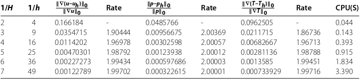
2 4 0.166184 - 0.0485766 - 0.0962505 - 0.044 3 9 0.0354715 1.90444 0.00956675 2.00369 0.0211715 1.86736 0.143 4 16 0.0114202 1.96978 0.00302598 2.00057 0.00682667 1.96713 0.393 5 25 0.00470301 1.98792 0.00123938 2.00012 0.00281136 1.98788 0.915 6 36 0.00227273 1.99434 0.000597686 2.00003 0.0013585 1.99451 1.834 7 49 0.00122789 1.99702 0.000322615 2.00001 0.000733929 1.99716 3.390
uses less time than the numerical schemes (.) and (.). From the above tables, we can see that the two-grid variational multiscale Oseen iterative method shows a good perfor-mance for the steady natural convection equations due to this scheme not only keeping a good accuracy but also taking the least computational cost.
5.2 Thermal driven cavity problem
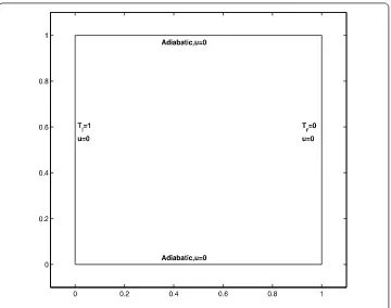
The problem of thermal driven cavity is used as a suitable benchmark for testing the nat-ural convection problem in the literature. The simplicity of the geometry and the clear boundary conditions make this test attractive. The domain consists of a square cavity with differentially heated vertical walls where the right and left walls are kept atTrandTl,
re-spectively, withTr>Tl. The remaining walls are insulated and there is no heat transfer
through them. The boundary conditions are no-slip boundary conditions for the veloc-ity at four walls (u= ) and Dirichlet boundary conditions for the temperature at vertical walls. As the horizontal walls are adiabatic, we employ∂T
∂n= . Figure shows the physical
domain of the thermal driven cavity flow problem. In this test, we follow the parameters set by Cibik and Kaya in [] and takek= ,b= ,Tl= , andTr= . While we consider the
so-Figure 1 The physical domain with its boundary conditions.
lution of [] and some other authors such as Cibik and Kaya [], Manzari [], and Wan
et al.[]. We also present the results of the standard Galekrkin FEM (.) where we keep the same mesh sizes for the two-grid variational multiscale method (.) and the one-grid variational multiscale method (.). Numerical simulations are obtained on the uniform grid ×. The mesh sizes of two-grid algorithms areH=andh=.
We start our illustrations by giving peak values of the vertical velocity aty= . and the horizontal velocity atx= .. Table summarizes the maximum vertical velocity values at mid-height and at mid-width for different Rayleigh numbers. We use SGFEM, OGVMM, TGVMM to denote standard Galerkin FEM, one-grid, and two-grid variational multiscale methods, respectively. For quantitative assessment, we include those velocity values ob-tained by [, , , ]. As can be observed, as the Rayleigh number takes values to
, the results of two-grid variational multiscale Oseen iterative method are in excellent
agreement with the benchmark data even at coarser gridH= .
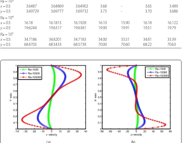
Next, we present the vertical and horizontal velocity at the mid-height and mid-width in Figure . It is obvious that as the Rayleigh numbers increase, the differences in the profiles provided in Figure are getting larger. These profiles are also comparable with a similar one in [, ]. Combining with Table , we can see that the two-grid variational multiscale Oseen iterative method is in good agreement with [, , , ].
Table 4 Comparisons of maximum velocity aty= 0.5 andx= 0.5 with different methods (h=641,H=18)
SGFEM OGVMM TGVMM Ref. [8] Ref. [5] Ref. [24] Ref. [25]
Ra = 103
x= 0.5 3.6487 3.64869 3.64902 3.68 - 3.65 3.489 y= 0.5 3.69729 3.69777 3.69732 3.73 - 3.70 3.686
Ra = 104
x= 0.5 16.18 16.1815 16.1928 16.10 15.90 16.18 16.122 y= 0.5 19.6244 19.6317 19.6381 19.90 19.91 19.51 19.79
Ra = 105
x= 0.5 34.7186 34.8201 34.7183 34.00 33.51 34.81 33.39 y= 0.5 68.4705 68.5433 68.5738 70.00 70.60 68.22 70.63
(a) (b)
Figure 2 Comparison of velocity at the mid-width with different Rayleigh numbers. (a)vertical velocity, (b)horizontal velocity.
(a) (b) (c) (d)
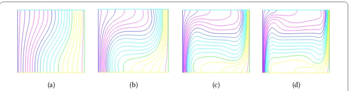
Figure 3 The streamlines of two level variational multiscale method for natural convection problem. (a)Ra = 103,(b)Ra = 104,(c)Ra = 105,(d)Ra = 5×10⁵.
as the thermal convection is concentrated. With the increase of Rayleigh numbers, the parallel behavior of temperature isolines is distorted as these lines seem to have a flat behavior in the central part of the region. Near the sides of the cavity, isolines tend to be vertical only. The temperature slopes withRa= ×at the corners of the differentially
(a) (b) (c) (d)
Figure 4 The isotherms of two level variational multiscale method for natural convection problem. (a)Ra = 103,(b)Ra = 104,(c)Ra = 105,(d)Ra = 5×10⁵.
Competing interests
The authors declare that no conflict of competing interests exists.
Authors’ contributions
XSM carried out the main theorem and checked this paper, ZZT wrote this article. XSM, ZZT, and TZ read and approved the final manuscript.
Author details
1Center for Intelligence Science and Technology, School of Computer Science, Beijing University of Posts and
Telecommunications, Beijing, 100876, P.R. China. 2School of Mathematics & Information Science, Henan Polytechnic
University, Jiaozuo, 454003, P.R. China.3Departamento de Matemática, Centro Politécnico, Universidade Federal do
Paraná, Curitiba, 81531-990, Brazil.
Acknowledgements
The authors are grateful to the editor and two referees for a number of helpful suggestions, which have greatly improved our original manuscript. This research is supported by CAPES and CNPq of Brazil (No. 88881.068004/2014.01), the NSF of China (No. 11301157), and the Foundation of Distinguished Young Scientists of Henan Polytechnic University (J2015-05).
Received: 20 December 2015 Accepted: 17 March 2016 References
1. Boland, J, Layton, W: An analysis of the finite element method for natural convection problems. Numer. Methods Partial Differ. Equ.2, 115-126 (1990)
2. Gresho, PM, Lee, M, Chan, ST, Sani, RL: Solution of time dependent, incompressible Navier-Stokes and Boussinesq equations using the Galerkin finite element method. In: Approximation Methods for the Navier-Stokes Problems. Springer Lecture Notes in Mathematics, vol. 771, pp. 203-222. Springer, Berlin (1980)
3. Boland, J, Layton, W: Error analysis for finite element methods for steady natural convection problems. Numer. Funct. Anal. Optim.11, 449-483 (1990)
4. Lenferink, HWJ: An accurate solution procedure for fluid flow with natural convection. Numer. Funct. Anal. Optim.15, 661-687 (1994)
5. Cibik, A, Kaya, S: A projection based stabilized finite element method for steady-state natural convection problem. J. Math. Anal. Appl.381, 469-484 (2011)
6. Galvin, KJ, Linke, A, Rebholz, LG, Wilson, NE: Stabilizing poor mass conservation in incompressible flow problems with large irrotational forcing and application to thermal convection. Comput. Methods Appl. Mech. Eng.237-240, 166-176 (2012)
7. Zhang, T, Zhao, X, Huang, PZ: Decoupled two level finite element methods for the steady natural convection problem. Numer. Algorithms68, 837-866 (2015)
8. Manzari, MT: An explicit finite element algorithm for convective heat transfer problems. Int. J. Numer. Methods Heat Fluid Flow9, 860-877 (1999)
9. Benítez, M, Bermúdez, A: A second order characteristics finite element scheme for natural convection problems. J. Comput. Appl. Math.235, 3270-3284 (2011)
10. Kaya, S, Layton, W, Riviere, B: Subgrid stabilized defect correction methods for the Navier-Stokes equations. SIAM J. Numer. Anal.44, 1639-1654 (2006)
11. Guermond, JL, Marra, A, Quartapelle, L: Subgrid stabilized projection method for 2D unsteady flows at high Reynolds numbers. Comput. Methods Appl. Mech. Eng.195, 5857-5876 (2006)
12. Layton, W: A connection between subgrid-scale eddy viscosity and mixed methods. Appl. Math. Comput.133(1), 147-157 (2002)
13. Zhang, Y, He, YN: Assessment of subgrid-scale models for the incompressible Navier-Stokes equations. J. Comput. Appl. Math.234, 593-604 (2010)
14. Galvin, KJ: New subgrid artificial viscosity Galerkin methods for the Navier-Stokes equations. Comput. Methods Appl. Mech. Eng.200, 242-250 (2011)
15. Hughes, TJR: Multiscale phenomena: Green’s functions the Dirichlet-to-Neumann formulation subgrid-scale models bubbles and the origins of stabilized methods. Comput. Methods Appl. Mech. Eng.127, 387-401 (1995)
16. John, V, Kaya, S: A finite element variational multiscale method for the Navier-Stokes equations. SIAM J. Sci. Comput. 26, 1485-1503 (2005)
18. Zheng, HB, Hou, YR, Shi, F, Song, LN: A finite element variational multiscale method for incompressible flows based on two local Gauss integrations. J. Comput. Phys.228, 5961-5977 (2009)
19. Layton, W, Lee, H, Peterson, J: A defect-correction method for the incompressible Navier-Stokes equations. Appl. Math. Comput.129, 1-19 (2002)
20. Liu, QF, Hou, YR: A two-level defect-correction method for Navier-Stokes equations. Bull. Aust. Math. Soc.81, 442-454 (2010)
21. Zhang, YZ, Hou, YR, Zheng, HB: A finite element variational multiscale method for steady-state natural convection problem based on two local Gauss integrations. Numer. Methods Partial Differ. Equ.30, 361-375 (2014)
22. Shang, YQ: A two-level subgrid stabilized Oseen iterative method for the steady Navier-Stokes equations. J. Comput. Phys.233, 210-226 (2013)
23. Hecht, F, Pironneau, O, Hyaric, A, Ohtsuka, K: http://www.freefem.org/ff (2008)
24. de Vahl Davis, D: Natural convection of air in a square cavity: a benchmark solution. Int. J. Numer. Methods Fluids3, 249-264 (1983)