R E S E A R C H
Open Access
The dynamics of a stage structure
population model with fixed-time birth pulse
and state feedback control strategy
Xiangsen Liu
1,2and Binxiang Dai
1**Correspondence:
1School of Mathematics and
Statistics, Central South University, Changsha, Hunan 410083, P.R. China Full list of author information is available at the end of the article
Abstract
In this paper, we study a stage structure population model with fixed-time birth pulse and state feedback control strategy. The stability of the trivial solution and the existence of periodic solutions are investigated. Sufficient conditions for the permanence of the system are obtained. Furthermore, some numerical simulations are given to illustrate our results. The superiority of the mixed control strategy is also discussed.
Keywords: stage structure; birth pulse; state feedback control strategy; periodic solution; permanence
1 Introduction
Stage structure models have attracted much attention in recent years. In most cases,
or-dinary differential equations are used to build stage structure models [, ]. However,
im-pulsive differential equations [, ] are also suitable for the mathematical simulation of evolutionary processes in which the parameters state variables undergo relatively long
periods of smooth variation followed by a short-term rapid change in their values. Many
results have been obtained for stage structure models described by impulsive differential
equations [–].
In most models, the increases in population due to births are assumed to be time-independent. However, many species give birth in a very short time. Caughley [] termed
this growth pattern a birth pulse. Thus, the continuous reproduction of population should
be replaced with a birth pulse. Liu and Chen [] investigated a two-species competitive
system with toxicant and birth pulse and obtained the existence of positive periodic
so-lutions. On the other hand, different kinds of impulsive effects were assumed to occur simultaneously in building models in most cases for simplicity. But different kinds of
im-pulsive effects occur at different moments in many practical problems. Recently, many
authors considered different kinds of impulsive effects that occur at different moments
[–]. In [], the authors considered the following model: spectively, andδ> is the maturity rate that determines the mean length of the juvenile period. A constant fraction –p( <p< ) of pest population is killed under the impulsive strategy at timet= nT,b> is the maximum birth rate,c=r(b–d),dis the maximum death rate, andris a parameter reflecting the relative importance of density-dependent population regulation through birth and death. Ifr= , then all density dependence acts through the death rate, and ifr= , then all density dependence acts through the birth rate.
In [], the authors addressed some problems on system (.) such as the existence and stability of positive period-Tsolutions and the existence of flip bifurcations by means of bifurcation theory.
In pest management, the pest population can be controlled by many methods, among which the fixed-time impulsive control strategy is widely performed in practice. However, this measure has some shortcomings, regardless of the growth rules of the pest and the cost of management. Another measure based on the state feedback control strategy is pro-posed in which the pesticide is sprayed only when the observed pest population reaches a certain threshold size. The latter measure is obviously more reasonable and suitable for pest control. Motivated by [], we consider the following model with fixed-time birth pulse and state feedback control strategy:
⎧
where the thresholdh> is a constant. When the amount of mature pests reaches the thresholdhat timeti(h), controlling measures are taken, and the amounts of the immature and mature pests abruptly turn topx(ti(h)) andpy(ti(h)), respectively.
Jianget al.[] investigated the periodic solutions and their relationship in an SIS epi-demic model with fixed-time birth pulses and state feedback pulse treatments. Linet al.
The remaining part of this paper is organized as follows. In the next section, we discuss the existence of positive periodic solutions of system (.). In Section , the stability of the trivial solution is considered. We study the permanence of system (.) in Section . In Section , some numerical simulations are given to illustrate our results. Finally, some concluding remarks are given.
2 The existence of periodic solutions
In this section, we investigate the existence of periodic solutions.
Set the initial point of system (.) asA(x,y) and suppose that the trajectory orig-inating from the initial point A reaches the liney(t) =hat the pointA(x,y) at time
By the second equation of system (.) we obtain
x=
h( –pexp(–dT))exp(dt)
–exp(–δt) +pexp(–dT)(exp(–δt) –exp(–δT))¯
Let
Theorem . Assume that condition(.)holds.Then there exists a period-T solution of
system(.)where the initial point(x∗,y∗)is as in(.).
A special period-T solution that is subject to spraying pesticide once, and birth pulse two times per period T is investigated in the following. Set the initial point of system (.) asA(x,y). The trajectory originating from the initial pointAreaches the point
Ifx+=x,y+=y, then the evolution of the dynamics repeats itself. For this to hold, lution of system (.) where the birth pulse occurs at the momentst=nT, whereas the pesticide is sprayed att= (n– )T+t. The initial point is (x¯,y¯). Then we obtain the following result.
Theorem . If the initial point(x,y) = (x¯,y¯),where(x¯,y¯)is the solution of (.),
then there exists a period-T solution of system(.).
3 The stability of the trivial solution
Now, we discuss the stability of the trivial solution of system (.). LetN(t) =x(t) +y(t). Then system (.) is equivalent to
(H) The trajectory originating from the initial pointAdoes not reach the liney(t) =h for <t≤T.
(H) The trajectory originating from the initial pointAreaches the liney(t) =honce at timeTfor <t≤T.
(H) The trajectory originating from the initial pointAreaches the liney(t) =honce at timetfor <t<Twhere <t<T.
(H) The trajectory originating from the initial pointAreaches the liney(t) =h k times for <t<T.
(H) It follows from system (.) that ify(t) <hfor <t≤T, then
(H) Suppose that the trajectory originating from the initial pointAreaches the line
y(t) =hat the pointA(N,y) fort=T. Then birth pulse occurs, and the pesticide is spayed. The trajectory jumps to the pointA+(N+,y+).
From system (.) we obtain
N+ =N+ (b–cN)y≤( +b)N= ( +b)Nexp(–dT)f(N).
(H) Suppose that the trajectory originating from the initial pointAreaches the line
y=hat the pointA(N,y) at timet=t, where <t<T, N =Nexp(–dt), and
y=h. Then the pesticide is spayed, and the trajectory jumps to the pointA+(N+,y+). The trajectory reaches the pointA(N,y) att=T and jumps toA+(N+,y+) due to the effect of birth pulse.
From system (.) we have
N+ =p(N–y) +py≤pN=pNexp(–dt).
So
N=N+exp
–d(T–t) ≤pNexp(–dt)exp
–d(T–t) =pNexp(–dT),
N+ =N+ (b–cN)y≤( +b)N= ( +b)pNexp(–dT)f(N).
(H) Suppose that the trajectory originating from the initial pointAreaches the line
y=hat the pointAn(Nn,yn) at timet=tn, where <tn<T, <n≤k, and jumps to the pointA+n(Nn+,yn+). The trajectory reaches the pointAk+(Nk+,yk+) att=T and jumps to the pointA+
k+(Nk++,y+k+) due to the effect of birth pulse. Similarly to the discussion of case (H), we have
Nk+≤pkNexp(–dT),
Nk++=Nk++ (b–cNk+)yk+≤( +b)Nk+≤( +b)pkNexp(–dT) f(N).
Hence, for <b<exp(dT) – ,
<f() < , <f() < , <f() < , <f() < .
Therefore,N(t) tends to zero withtincreasing for <b<exp(dT) – . SoN(t) <(δ+dδ)h over a limited period of time for any initial point (N,y). It is seen from (.) that
dy
dt=δN– (δ+d)y<
if N< (δ+dδ)h, y> h, which means that the trajectory of system (.) will enter region
of mature pests is small (less than the threshold levelh). It follows from system (.) that to the above analysis, we get
⎧
Then the following map is obtained:
Nn+= ( +b)Nnexp(–dT) –cNnexp(–dT),
yn+= (exp(–dT) –exp(–(δ+d)T))Nn+ynexp(–(δ+d)T).
(.)
There exists a fixed pointA¯(, ) of map (.). The associated characteristic polynomial of the fixed pointA¯ of map (.) is given by pointA¯(, ) of map (.) is locally asymptotically stable. Hence, the trivial solution of system (.) is locally asymptotically stable for <b<exp(dT) – , which is given in the following result.
Theorem . The trivial solution of system(.)is locally asymptotically stable for <b<
exp(dT) – .
4 Permanence
In the following, we discuss the permanence of system (.) by means of system (.) and assume thatc> . We set the initial point of system (.) asA(N,y) where <y<h. Two cases are considered.
(E) The trajectory originating from the initial pointAdoes not reach the liney(t) =h for <t≤T.
(E) The trajectory originating from the initial pointAreaches the liney(t) =hat time
(E) It follows from system (.) that
NT+ =N(T) +b–cN(T) y(T)
=Nexp(–dT) +bNexp(–dT) –b(N–y)exp
–(δ+d)T
–cNexp(–dT) +cNexp(–dT)(N–y)exp
–(δ+d)T
>N
( +b)exp(–dT) –bexp–(δ+d)T –cNexp(–dT)
.
Suppose ( +b)exp(–dT) –bexp(–(δ+d)T) > . Then there exists> such that ( +
b)exp(–dT) –bexp(–(δ+d)T) > +. Thus,N(T+) > ( +)Nif
<N<
exp(dT)
c
+b–bexp(–δT) – ( +)exp(dT)D. (.)
Assume that
δD– (δ+d)h< . (.)
Then there exists> small enough such thatδD– (δ+d)( –)h< . From (.) we obtain
dy
dt=δN– (δ+d)y<δD– (δ+d)( –)h< forN<D,y> ( –)h.
Thus,y(t) <hifN(t) <Dfor allt> . IfN(t) <Dfor <t≤nT, then
NnT+ ≥( +)N(n– )T+ ≥( +)nN. (.)
It follows from (.) that there existsn> such thatN(nT+) >D. In this case, there exists t > , wherenT <t< (n+ )T, such thaty(t) =handN(t)≥D. Then the pesticide is sprayed. Letp¯=min{p,p}. Then
Nt+ =px(t) +py(t)≥ ¯pN(t).
We need to consider the following two cases. () N(t+)≥D.
() N(t+ ) <D.
() IfN(t+)≥D, then, similarly to the above analysis, there existst<t< (n+ )Tsuch thaty(t) =handN(t+
)≥ ¯pN(t). ForN(t+)≥D, we may continue the same argument. ForN(t+) <D, by the first equation of system (.) we find
N(t) <Nt+ <D fort<t< (n+ )T.
Theny(t) <hfort<t< (n+ )T. Thus,
N(n+ )T =N
t+ exp–d(n+ )T–t
Sincey(t) =h, from the above discussion we get
N(t) >D.
ThenN((n+ )T)≥ ¯pDexp(–dT). It is easy to see that the birth pulseN((n+ )T) > ; thenN((n+ )T+)≥N((n+ )T). It is possible thatN((n+ )T+)≥D. It is well known that this case coincides with the caseN(t+)≥D, and therefore we omit it.
From the above analysis we get
N(t)≥N(n+ )T ≥ ¯pDexp(–dT) fornT<t≤(n+ )T. IfN((n+ )T+) <D, then we have
N(n+ )T =N
(n+ )T+ exp(–dT)≥N
(n+ )T exp(–dT)
≥ ¯pDexp(–dT)m. (.)
Therefore,N(t)≥mfornT<t< (n+ )T. SinceN((n+ )T+) <D, we obtainN((n+ )T+)≥N((n+ )T+). ForN((n+ )T+)≥D, this case coincides withN(t+)≥D. For
N((n+ )T+) <D, we obtain
N(n+ )T =N
(n+ )T+ exp(–dT)≥N
(n+ )T+ exp(–dT)≥m. Hence,
N(t) >N(n+ )T ≥m for (n+ )T<t≤(n+ )T. Continuing the same argument, we getN(t)≥mfort>nT.
() IfN(t+
) <D, then we find
N(n+ )T =N
t+ exp–d(n+ )T–t
≥ ¯pN(t)exp(–dT)
≥ ¯pDexp(–dT).
From the first and fifth equations of system (.) we have
N(t)≥N(n+ )T ≥ ¯pDexp(–dT) >m fornT<t≤(n+ )T.
It is easy to see thatN((n+ )T+)≥N((n+ )T). IfN((n+ )T+)≥D, it is well known that the case coincides with case (). ForN((n+ )T+) <D, we obtain
N(n+ )T+ ≥N
(n+ )T =N
(n+ )T+ exp(–dT)
≥N(n+ )T exp(–dT)≥ ¯pDexp(–dT).
From the first and fifth equations of system (.) we get
SinceN((n+)T+) <D, we obtainN((n+)T+)≥N((n+)T+). ForN((n+)T+)≥D, this case coincides with case (). ForN((n+ )T+) <D, we obtain
N(n+ )T =N
(n+ )T+ exp(–dT)≥N
(n+ )T+ exp(–dT)
≥ ¯pDexp(–dT) =m.
Hence,
N(t) >N(n+ )T ≥m for (n+ )T<t≤(n+ )T.
Continuing the same argument, we getN(t)≥mfort>nT. (E) In this case, we have
y(t) =h for <t≤T.
By case (E) we obtain
N(t) >D.
Similarly to the discussion of case (), that is,N(t+
) >D, it is easy to see thatN(t) >mfor large enought> .
In conclusion, for any initial valueN> , there existst> such thatN(t)≥m for
t>t.
Ify(t) =hfor <t<T, then
N(t) = –N(t) +p
N(t) –y(t) +py(t)≤–N(t) +pN(t).
Thus,N(t+)≤pN(t) <N(t). Then the number of the total pests is decreasing when the pesticide is spayed. Therefore,N(T)≤Nexp(–dT).
In view of the birth pulseN= (b–cN)N> , it is easy to see thatb–cN(T)≥b–
cNexp(–dT) > , that is,N<bexpc(dT). From the first and fifth equations of system (.) we get
N(t)≤N<
bexp(dT)
c for <t≤T.
It is easy to see that
NT+ =N(T) +b–cN(T)y(T)≤N(T) +b–cN(T) N(T)
≤–cN(T) + ( +b)N(T)≤( +b)
c .
It is well known that
N(T)≤NT+ exp(–dT)≤( +b)
In view of the birth pulseN(T) = (b–cN(T))N(T) > , we get
N(T) <b
c.
For this to hold, the following condition is satisfied;
( +b)
c exp(–dT) < b
c, that is, ( +b)
≤bexp(dT).
From the first and fifth equations of system (.) we obtain
N(t)≤NT+ ≤( +b)
c forT<t≤T.
It is easy to see that
NT+ =N(T) +b–cN(T) y(T)≤N(T) +b–cN(T) N(T)
≤–cN(T) + ( +b)N(T)≤( +b)
c .
From the first and fifth equations of system (.) we get
N(t)≤NT+ ≤( +b)
c for T<t≤T
and
N(T) <NT+ exp(–dT)≤( +b)
c exp(–dT)≤ b c.
It is well known that
NT+ =N(T) +b–cN(T) y(T)≤N(T) +b–cN(T) N(T)
≤–cN(T) + ( +b)N(T)≤( +b)
c .
Continuing the same argument, we obtain
N(t)≤( +b)
c fornT<t≤(n+ )T.
Let
M=max
bexp(dT)
c ,
( +b) c
. (.)
Thus, for any initial value <N<bexpc(dT) andt> ,
Therefore, for large enought> ,
m≤N(t)≤M. (.)
Now we consider the persistence of the mature pest populations. It follows from (.) that there existst> such thatN(t)≥mfort>t. Thus, from system (.) we have
dy
dt=δN– (δ+d)y≥δm– (δ+d)y fort>t.
In the following, we consider three cases. ()ph<δδm+d <h.
It is easy to see that for large enought> andy<δm δ+d,
dy
dt≥δm– (δ+d)y> .
Hence, for large enought> ,ph≤y(t)≤h. () δm
δ+d≤ph.
It is well known that for large enought> ,δm
δ+d≤y(t)≤h.
() δm δ+d≥h.
For large enought> andy≤h,
dy
dt≥δm– (δ+d)y> .
Thus, for large enought> ,ph≤y(t)≤h.
In conclusion, for large enought> ,m≤y(t)≤h, where
m=min
ph,
δm
δ+d
. (.)
Then we obtain the following result.
Theorem . Assume that condition(.)holds,c> , ( +b)≤bexp(dT), and( +
b)exp(–dT) –bexp(–(δ+d)T) > .Then for any initial point A(x,y)in system(.)such
that <x+y< bexpc(σT) and <y≤h,there exists¯t> such that m≤x(t) +y(t)≤
Mand m≤y(t)≤h for t>t¯,where m,M,and mare given in(.), (.),and(.),
respectively.
The particular casec= is investigated as follows. Set the initial point of system (.) as
¯
A(x,y) with <y<h. We consider two cases.
(B) The trajectory originating from the initial pointAdoes not reach the liney(t) =h for <t≤T.
(B) The trajectory originating from the initial pointAreaches the liney(t) =hat time
twhere <t≤T.
(B) It follows from system (.) that
xT+ =xexp
–(δ+d)T +b(x+y)exp(–dT) –bxexp
–(δ+d)T
>xexp
–(δ+d)T +bxexp(–dT) –bxexp
It is well known thatx(T+) >x if
–b+bexp(δT) –exp(δ+d)T > . (.)
From system (.) we have
dy
dt=δx–dy< forx< dph
δ ,y>ph.
Thus,
y(t) <h ifx(t) <dph
δ for allt> .
By (.) it is easy to see that there exists> such that
–b+bexp(δT) –exp(δ+d)T >,
that is,
exp–(δ+d)T +bexp(–dT) –bexp–(δ+d)T > +.
Hence,
xT+ >x( +).
Ifx(t) <dph
δ for <t≤nT, then
xnT+ ≥( +)x(n– )T+ ≥( +)nx. (.)
It follows from (.) that there existsn> such thatx(nT+) >dpδh. Similarly to the case
c> , there existst> such that, fort>t,
x(t) >dph
δ exp
–(d+δ)T m¯. (.)
(B) In this case, we get
y(t) =h for <t≤T. By case (B) we obtain
x(t) >dph
δ .
Similarly to the discussion of case (B), it is easy to see thatx(t) >m¯for large enought> . By system (.) we obtain
dy
In the following, we discuss three cases.
Then we obtain the following result.
Theorem . Assume that condition(.)holds and c= .Then for any solution of system
(.),there exists t∗> such thatm¯≤x(t)andm¯≤y(t)≤h for t>t∗,wherem¯andm¯
are given in(.)and(.),respectively.
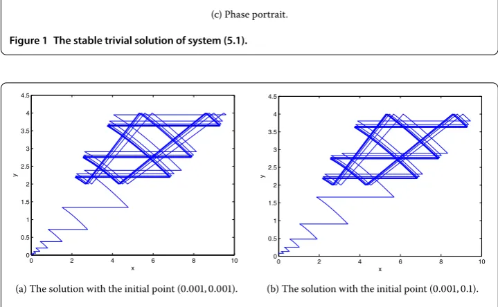
5 Numerical simulation with the initial point (, .) is shown in Figure . It is seen that the solution tends to the trivial solution withtincreasing, which means that the trivial solution is asymptotically stable.
5.2 Species persistence
(a) Time series ofx. (b) Time series ofy.
(c) Phase portrait.
Figure 1 The stable trivial solution of system (5.1).
(a) The solution with the initial point (., .). (b) The solution with the initial point (., .).
Figure 2 The solutions of system (5.1) withc= 0.2.
the trajectory of system (.) enters a quadrilateral and stays in it forever, which verifies Theorem ..
(a) The solution with the initial point (., .). (b) The solution with the initial point (., .).
Figure 3 The solutions of system (5.1) withc= 0.
(a) Time series ofx. (b) Time series ofy.
(c) Phase portrait.
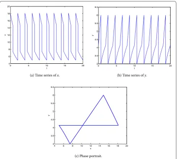
Figure 4 The period-Tsolution of system (5.1) withh= 6,b= 5,p1=p2= 0.5, and the initial point
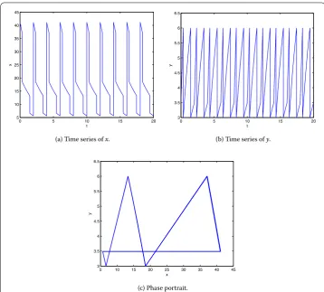
(a) Time series ofx. (b) Time series ofy.
(c) Phase portrait.
Figure 5 The period-Tsolution of system (5.1) withh= 6,b= 12,p1=p2= 0.5, and the initial point
(41, 3.5).
5.3 The existence of periodic solutions
Seth= ,b= ,p=p= .. The phase portrait and time series ofxandyof system (.) with the initial point (, .) are shown in Figure , wheret= .. It is seen that
y(t) reaches the threshold valuey(t) = att= n– +t, wheren= , , . . . . The pulse treatment and birth pulse occur att= n– +tandt= n, respectively. Then system (.) has a period-Tsolution, which verifies Theorem ..
Seth= ,b= ,p=p= .. The phase portrait and time series ofxandyof system (.) with the initial point (, .) are shown in Figure , wheret≈.,t≈.. It is seen thaty(t) reaches the threshold valuey(t) = att= n– +tandt= n– +t, respectively, wheren= , , . . . . The pulse treatment occurs att= n– +tandt= n– +t, respectively. The birth pulse occurs at t= n. Then system (.) has a period-T
solution.
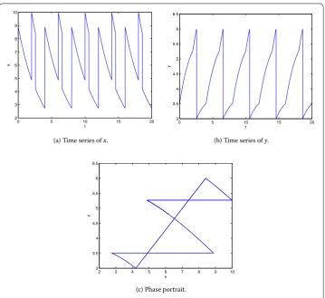
Seth= ,b= ,p=p= .. The phase portrait and time series ofxandyof system (.) with the initial point (., .) are shown in Figure , wheret≈.. It is seen that
(a) Time series ofx. (b) Time series ofy.
(c) Phase portrait.
Figure 6 The period-2Tsolution of system (5.1) withh= 6,b= 3,p1=p2= 0.5, and the initial point
(8.9, 3.5).
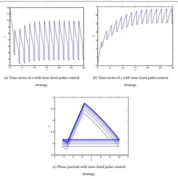
5.4 The superiority of the mixed control strategy
Setd= .,δ= .,T= ,c= .,h= ,b= ,p= .,p= ., and the initial point (, .) in system (.). The system of the time-fixed pulse control strategy
⎧ ⎪ ⎪ ⎪ ⎪ ⎪ ⎪ ⎪ ⎪ ⎪ ⎨ ⎪ ⎪ ⎪ ⎪ ⎪ ⎪ ⎪ ⎪ ⎪ ⎩
x(t) = –.x– .x,
y(t) = .x– .y,
t=n,n= , , , . . . ,
x(t) = –( –p)x,
y(t) = –( –p)y,
t= n– ,
x(t) = (b–c(x+y))y,
y(t) = ,
t= n,
(.)
and the state feedback control strategy
x(t+) =px,
y(t+) =p y,
y(t) = ,
are shown in Figure and Figure , respectively, where ≤t≤.
(a) Time series ofxwith time-fixed pulse control
strategy.
(b) Time series ofywith time-fixed pulse control
strategy.
(c) Phase portrait with time-fixed pulse control
strategy.
Figure 7 The solution of system (5.2) withh= 6,b= 3,p1= 0.7,p2= 0.75, and the initial point (12, 0.1).
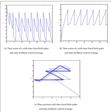
seven times in the case of state feedback control strategy, andy(t) is controlled under the threshold valueh= . In view of the total number of spraying pesticide and results of two control strategies, the state feedback control strategy is more effective than the time-fixed pulse control strategy.
6 Conclusion
(a) Time series ofxwith time-fixed birth pulse
and state feedback control strategy.
(b) Time series ofywith time-fixed birth pulse
and state feedback control strategy.
(c) Phase portrait with time-fixed birth pulse
and state feedback control strategy.
Figure 8 The solution of system (5.1) withh= 6,b= 3,p1= 0.7,p2= 0.75, and the initial point (12, 0.1).
Competing interests
The authors declare that they have no competing interests.
Authors’ contributions
All authors contributed equally to the writing of this paper. All authors read and approved the final manuscript.
Author details
1School of Mathematics and Statistics, Central South University, Changsha, Hunan 410083, P.R. China.2Department of
Mathematics, North University of China, Taiyuan, Shanxi 030051, P.R. China.
Received: 11 September 2015 Accepted: 29 April 2016
References
1. Hastings, A: Age-dependent predation is not a simple process. I. Continuous models. Theor. Popul. Biol.23, 347-362 (1983)
2. Aiello, WG, Freedman, HI: A time delay model of single-species growth with stage structure. Math. Biosci.101, 139-153 (1990)
3. Laksmikantham, V, Bainov, DD, Simeonov, PS: Theory of Impulsive Differential Equations. World Scientific, Singapore (1989)
4. Bainov, DD, Simeonov, PS: Impulsive Differential Equations: Periodic Solutions and Applications. Longman, New York (1993)
5. Zhang, H, Chen, L, Nieto, JJ: A delayed epidemic model with stage-structure and pulses for pest management strategy. Nonlinear Anal., Real World Appl.9, 1714-1726 (2008)
6. Jiang, G, Liu, Q, Peng, L: Impulsive ecological control of a stage-structured pest management system. Math. Biosci. Eng.2(2), 329-344 (2005)
7. Shi, R, Chen, L: Staged-structured Lotka-Volterra predator-prey models for pest management. Appl. Math. Comput.
203, 258-265 (2008)
9. Liu, Z, Chen, L: Periodic solution of a two-species competitive system with toxicant and birth pulse. Chaos Solitons Fractals32, 1703-1712 (2007)
10. Liu, B, Duan, Y, Luan, S: Dynamics of an SI epidemic model with external effects in a polluted environment. Nonlinear Anal., Real World Appl.13, 27-38 (2012)
11. Zhao, Z, Zhang, XQ, Chen, LS: The effect of pulsed harvesting policy on the inshore-offshore fishery model with the impulsive diffusion. Nonlinear Dyn.63, 537-545 (2011)
12. Zhang, H, Georgescu, P, Chen, LS: On the impulsive controllability and bifurcation of a predator-pest model of IPM. Biosystems93, 151-171 (2008)
13. Georgescu, P, Morosanu, G: Pest regulation by means of impulsive controls. Appl. Math. Comput.190, 790-803 (2007) 14. Nie, L, Peng, J, Teng, Z, Hua, L: Existence and stability of periodic solution of a Lotka-Volterra predator-prey model
with state dependent impulsive effects. J. Comput. Appl. Math.224, 544-555 (2009)
15. Wu, X: Bifurcation of nontrivial periodic solutions for an impulsively controlled pest management model. Appl. Math. Comput.202, 675-687 (2008)
16. Ma, Z, Yang, J, Jiang, G: Impulsive control in a stage structure population model with birth pulses. Appl. Math. Comput.217, 3453-3460 (2010)
17. Jiang, G, Liu, S, Ling, L: Periodic solutions of a SIS epidemic model with fixed-time birth pulses and state feedback pulse treatments. Int. J. Comput. Math.91, 844-856 (2014)