A neural data driven algorithm for smart sampling in wireless sensor networks

(1)

R E S E A R C H

Open Access

A neural data-driven algorithm for smart

sampling in wireless sensor networks

Luca Mesin

*

, Siamak Aram and Eros Pasero

Abstract

Wireless sensor networks (WSN) take on an invaluable technology in many applications. Their prevalence, however, is threatened by a number of technical difficulties, especially the shortage of energy in sensors. To mitigate this problem, we propose a smart reduction in data communication by sensors. Indeed, in case we have a solution to this end, the components of a sensor, including its radio, can be turned off most of the time without noticeable influence on network operation. Thus, reducing the acquired data, the sensors can be idle for longer and power can be saved. The main idea in devising such a solution is to minimize the correlation between the data communicated. In order to reduce the measurements, we present a data prediction method based on neural networks which performs an adaptive, data-driven, and non-uniform sampling. Evidently, the amount of possible reduction in required samples is bounded by the extent to which the sensed data is stationary. The proposed method is validated on simulated and experimental data. The results show that it leads to a considerable reduction of the number of samples required (and hence also a power saving) while still providing a good approximation of the data.

Keywords:Data-driven sampling; Energy consumption; Neural data prediction; Sensor networks

1 Introduction

Wireless sensor networks (WSN) have received a great at-tention in recent years. They have a wide variety of applica-tions such as event detection, target tracking, environment sensing, elder people monitoring, and security [1-8]. A WSN is usually made up of a large number of sensors that communicate their sensed information to other nodes. Sensors are often supplied with scarce energy resources. Hence, energy saving is crucial to the operation of WSNs, and devising methods for efficient power consumption is central to the research in this area.

Studies show that the communication component of a sensor consumes more power than the computational unit and that power consumption is in minimum in the sleep state of the radio communication [9].

Many approaches were proposed to reduce the power consumption of a sensor network, but the following three main techniques are the most important among them [9,10]: duty cycling, data-driven approaches, and mobility. Since duty cycling patterns are unaware of data which are

gathered from sensor nodes, data-driven approaches are more appropriate to reduce the energy consumption of the WSNs.

The microcontroller can switch on the sensors only dur-ing the measurement, reducdur-ing the power consumption [4,5]. Nevertheless, unneeded communications could spor-adically happen because of transferring unnecessary data. Reducing extra communications is a way to save energy which can be followed by data-driven techniques. While ‘energy-efficient data acquisition’schemes are mainly con-cerned with decreasing power consumption relevant to the sensing subsystem, ‘data reduction’ schemes focus on unneeded samples.

In this paper, data prediction is employed. This work has been partially presented in IEEE WSCAR 2014 [11,12]. An innovative method is proposed and tested on simulated and experimental data. A neural algorithm is considered to forecast sensor measurements and their uncertainties to allow the system to reduce communications and transmit-ted data. In particular, a multilayer perceptron (MLP) net-work [13] is used. The central control unit selects when and from which sensor to acquire a new sample, without scheduling a periodical sampling. In the period between * Correspondence:[email protected]

Department of Electronics and Telecommunications, Politecnico di Torino, Turin 10129, Italy

(2)

two acquisitions, there are no transmissions in order to save energy.

2 Methods

2.1 Algorithm for efficient sampling

To reduce the number of acquired data, we predicted them and estimated the uncertainty of the prediction. An additional measurement was required from a sensor when the associated uncertainty went above a threshold.

Each available measurement was considered together with its uncertainty, assumed to be equal to the accuracy of the sensor. A MLP was used to perform periodically a forward prediction on 100 realizations of stochastic in-puts extracted from a uniform probability distribution with mean and range given by the available data and their uncertainty, respectively (see Appendix 1 for details on the MLP). The prediction was computed as the mean of the obtained 100 estimations. The uncertainty of the predictionUwas defined in terms of two contributions. The first was the dispersion of the predictions, indicated in the following as U1and defined as the range of the

estimations provided by the MLP from the 100 random trials. The second contribution U2 was the estimated

rate of prediction error:

Wherepjandmjindicate the jth predicted and measured value, respectively (so that |pj−mj| is the prediction error),τjis the time sample in which the jth measurement is taken (so thatτj−τj−1is the time delay between the jth

and the previous measurement). Thus,U2is the mean of

the last two estimated ratios between the prediction error and the time delay from the last measurement (so that the estimated rate of increase of prediction error has a mem-ory term). A convex combination of the two contributions was considered as the definition of the uncertainty

U¼αU1þð1−αÞU2 ð2Þ

where the parameter α (with 0 <α< 1) weights the im-portance of the two mentioned contributions. In the following, the same algorithm is tested on different data-sets (refer to Section2.2). For such general applications, there is no reason to give more importance to one of the two contributions in Equation2, so that αis considered 0.5 in the following. However, for specific applications, a different weight could be optimal.

A new acquisition was required from a sensor when the uncertainty of the predicted measurement was larger than a threshold (which was chosen as sensor specific). Thus, the MLP was used to estimate when and from which sensor to acquire a measurement. This allows to

reduce the number of measurements and, consequently, also the power consumption (as there is a decline on communication, the energy is saved by decreasing the number of transmissions). After acquiring a measure-ment from a sensor, its present and past data were up-dated by interpolating the acquired measurements and their uncertainties were updated according to the accur-acy of the sensor.

2.2 Data test bed

Both simulated and experimental data were used to test the algorithm.

2.2.1 Simulated data

Simulated data were deterministic and noise free. Two different simulations were considered. The first one in-volved the following two signals

x1ð Þ ¼t sin 2ð πf tð ÞtÞ

x2ð Þ ¼t a tð Þx1ð Þt ð3Þ

wheretis the time (in the range of 0 to 200 s, sampled at 20 Hz), f(t) is a square wave varying between 0.5 and 1.0 Hz with period 20 s anda(t) = 4 + sin(0.15πt). The sig-nals were quantized in order to have resolution 0.05 (also considered as the accuracy of the measurement). The two signalsx1andx2were first used separately, then together.

As the second set of simulations, two uncorrelated sig-nals were considered and sampled every 0.1 s for 60 min. The first signal is a sinusoid with frequency 0.1 Hz, and the second is defined as the first componenty1of the

solu-tion [y1y2y3] of a Lorenz system in chaotic regime [14]:

The signals were quantized in order to have reso-lution 0.1.

2.2.2 Experimental data

Two different experimental data were considered. The first dataset was constituted of meteorological data acquired every 15 min from four sensors, measuring temperature, pressure, wind velocity, and humidity, located at the Turin-Caselle airport, for 100 days from June to August 2010 (refer to [15] for details).

(3)

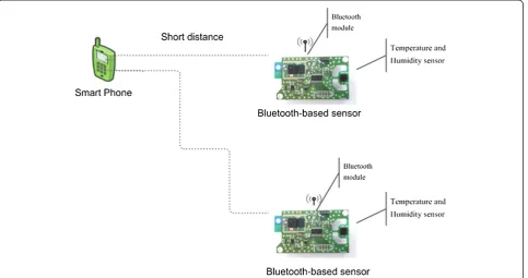
F2M03GLA from Free2Move was attached to the device. It consumes about 44 mW when it is waiting for connec-tion and 108 mW during the transmission. Data is re-ceived from the UART interface of the microcontroller by the bluetooth module and forwards it to a receiver using the serial port profile (SPP) service. The device is powered by a 3-V lithium battery (CR2247 from Motorola) with 1,000 mAh. The sensors were fixed on a carrier, and their location was changed irregularly and sequentially in three different locations in a laboratory: close to a cold or to a warm source and far from heat sources. The sources were sufficient to prompt changes on temperature and humid-ity up to 5°C and 10%, respectively. Data were recorded every 15 s for about an hour.

3 Result

Figures 2 and 3 show the application of the method to sim-ulated signals (see Section 2.2.1). In Figure 2, correlated non-stationary signals are considered. As shown in panel A, the method using the combination of the two signals has a lower slope of the reduction ratio versus estimation error. This indicates higher performances when informa-tion is jointly extracted from the two correlated signals. Moreover, the method selects more samples for the por-tions of the signals with higher frequency (Figure 2B), showing the ability to adapt in time to temporal variations of the signal.

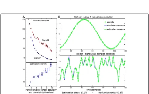
In Figure 3, the sinusoidal and the chaotic signals are considered. As expected, the prediction of the sinusoid

is simpler than that of the chaotic signal; for this reason, more measurements are selected by the algorithm to sam-ple appropriately the second signal (as shown in panel A).

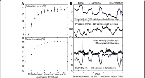
In Figure 4, a representative example application for our algorithm to our first bunch of experimental data is shown (meteorological data, Section 2.2.2). The MLP was trained and validated on the basis of the first 80 days (see Appendix 1). Then, it was applied on the following 20 days considered in Figure 4 (test set). In panel A, we show the results of many applications of the prediction algorithm to the test experimental data, with different thresholds. As expected, by increasing the threshold, the reduction factor increases, at the expense of decreasing the accuracy in estimating the measurements. In panel B, a portion of the test data is shown. Note that the number of samples required from the wind velocity sen-sor is the highest among the four sensen-sors, reflecting the erratic dynamics of the signal. On the other hand, the sampling of humidity, which has smooth variations cor-related with temperature, has the lowest rate.

(4)

Figure 2Application of the method to non-stationary,correlated signals (see Section 2.2.1). (A)Relation between reduction ratio and error (100 simulations with different thresholds are considered).(B)Samples for the portions of the signals with higher frequency versus those with lower frequency (same 100 simulations as inA).(C)Representative example application for the method.

Figure 3Application of the algorithm to simulated data (see Section 2.2.1). (A)Number of samples and mean estimation error (mean and standard deviation over ten repetitions).(B)Representative example (threshold = 0.03 for both signals).

(5)

Again, by increasing the threshold, the reduction factor increases and the accuracy in estimating the measure-ments decreases.

4 Discussion

This paper investigates the possibility of reducing the amount of communications and subsequently the power consumption of a sensor network by a smart sampling of data. Since reading from a bluetooth-based acquisi-tion system is one of the most expensive task in terms of power consumption in WSNs, energy saving can be ob-tained by timely replacing read data with predicted data. Reducing the number of measurements could be benefi-cial also in general networks, in order to save power or memory. An innovative and general method is discussed in this paper to determine when and which sensor to interrogate. It is based on a data prediction approach. Data prediction is also applied in [16], where data are pre-dicted and streamed only when the mismatch with respect to the acquired measurement is higher than a threshold. A similar approach is used in [17], where Kalman filters are applied for the prediction. These methods are more useful to conserve bandwidth than to reduce battery consumption. Indeed, the sensors waste energy to per-form the prediction and a continuous sampling, so that they cannot be switched off, but the computational load and cost of each node are increased. On the other hand,

only the base station is used in [18] to perform the prediction, not the nodes. However, the sensors are periodically interrogated to test if the predicted value is sufficiently accurate. Another method to reduce power consumption of a WSN is data aggregation [19]. It is an application-specific technique that is considered in most cases in which data are transferred between intermedi-ate or neighboring nodes.

The proposed algorithm estimates a prediction uncer-tainty for each sensor in the network during the monitoring. A specific sensor is interrogated when its uncertainty is above a threshold, which can be selected by the user (allowing, for example, to fit better a spe-cific dataset or to impose a deeper undersampling of a sensor). The algorithm to estimate the sensor uncer-tainties is based on a tool for data forecasting. It is used to estimate the rate of increasing of the prediction error and the future dispersion of the predictions due to the uncertainty contained in the available data (due to the finite precision of the sensors or the errors cumulated by iterating the prediction). Two contributions (related to the predicted errors and to the dispersion of the pre-dictions) are given the same weight and linearly com-bined for the estimation of the uncertainty associated to the sensor.

The method was tested on both simulated and experi-mental data. Simulated data were examined to analyze Figure 4Application of the algorithm to meteorological experiments (see Section 2.2.2).Accuracy is assumed to be 0.2°C, 20 hPa,

(6)

the algorithm correctness. Different simulations were considered, in order to analyze the following properties:

1. The performance of the proposed method on non-stationary signals

2. The ability of integrating the information from correlated measurements

3. The management of chaotic versus periodic signals

Our method adapted the sampling rate to the properties of a non-stationary signal, so that more samples were re-quired for the portions of the signal with higher frequency. Moreover, when applied to two correlated signals, the method improved the performances with respect to the case in which it was applied on the two signals separately. Finally, the method required more samples to describe a chaotic system than a simple periodic one. All these sults are in line with our expectations and confirm the re-liability of the proposed method.

Two applications to experimental data are also pro-vided. When applied to meteorological data, the method

was able to reduce the number of acquired samples with low estimation errors. More samples were recorded from the sensor monitoring the wind velocity, which provided a very erratic signal, with respect to temperature, pres-sure, and humidity, which showed regular and correlated variations. Notice that only a representative application is here considered: for practical applications, as only aver-age information on wind velocity is usually of interest, subsequent measured or estimated samples could be aver-aged, reducing further the data to be effectively transmit-ted. This outdoor application is in line with the results of the application of our method to indoor environmental data from a WSN.

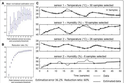
Considering the power consumed by the sensors dur-ing transmission and when in the idle state, some con-siderations could be made on the power that could be saved using our algorithm to reduce the number of measurements (see Appendix 2). Considering the in-door application, a reduction of the 50% of samples (getting an estimation error of about 35%, see Figure 5) allows to decrease the power consumption of about Figure 5Application of the algorithm to indoor experiments (see Section 2.2.2). (A)Root mean square (RMS) estimation error, and(B)

reduction ratio as functions of the uncertainty threshold (assumed proportional to sensor accuracy; the method was run 100 times for each choice of the threshold, mean and standard deviations are shown). The accuracy was assumed to be 0.1°C and 0.3%, for the T and H sensors, respectively.(C)Representative example application for our method: uncertainty of the measurements was assumed to be two times the accuracy.

(7)

7.5%; for the outdoor application here considered, data could be reduced to 70% (guaranteeing an estimation error lower than 20%, see Figure 4); thus, by scaling the acquisition and sampling times, a 10% of power saving could be obtained.

The results of the application of our method appear to be promising, even if a basic and general method was considered. Following the same ideas, more sophisti-cated methods could be developed, in order to better fit specific applications. For example, only the last two (measured or predicted) samples are here considered as the inputs of the prediction algorithm. This choice is due to the general applications discussed here, where four different datasets were processed by the same algo-rithm. However, different inputs can be chosen (e.g., the average values of data on long periods, often used in me-teorological forecasting applications, or delayed samples with an optimally chosen delay, or simply more than two values could be used from each sensor; the methods of time series embedding [20] could be used to support a proper selection of the optimal delay and of the num-ber of delayed values to characterize better each sensor). Moreover, a simple MLP was used for data prediction (see Appendix 1). Different alternative methods could be applied instead but still following the main general ideas of this paper. For example, different neural networks or fuzzy rule-based systems can be used [21]. Also, a single MLP is used here to predict all the measurements of the sensors, but different MLPs could be used, one for each sensor. The method estimates the uncertainty of the predicted measurements as the average of two contribu-tions: different combinations can fit specific applications better. Moreover, a linear increase of the prediction error, including a memory term, is here assumed, but a more sophisticated (nonlinear, adaptive) algorithm can be introduced in the future to estimate better the raise of the prediction error in time.

5 Conclusions

This paper introduces an innovative method to make a smart sampling from sensors, in order to avoid unneeded measurements and, consequently, to reduce power con-sumption. The main innovation is the proposed method-ology: using an intelligent system that predicts data and the uncertainty of the estimation in order to select an op-timal sampling. Different variants can be proposed in the future to fit specific applications.

Appendices

Appendix 1 Prediction algorithm

A set of MLPs is considered to perform the prediction. Measurements from each sensor were interpolated at a constant time interval τ. The value of the interpolated measurement in the most recent time and the delayed

value of one sample interval are considered for each sensor as the inputs of the MLP. The data are divided into training (60% of data), validation (20% of data), and test sets (20% of data). A single hidden layer is used, which is sufficient to approximate any nonlinear function (universal approximation property, [22]). The neurons in the hidden layer applies a sigmoidal activa-tion funcactiva-tion

f xð Þ ¼ð1þ expð Þ−x Þ−1 ð5Þ

The number of neurons in the hidden layer is chosen in the range from 20 to 50. The output neurons have linear activation function. Each output neuron is used to predict the measurement of a specific sensor. MLPs are trained by modifying iteratively the weights and the bias in order to reduce the error in predicting the training data, applying the quasi-Newton algorithm [13] for a number of iterations in the range of 50 to 400 times. An optimal network is se-lected choosing the topology (i.e., the number of hidden neurons) and the parameters (synaptic weights and bias, after a specific number of iterations of the optimization al-gorithm) with best generalization performances (i.e., with minimum error in the validation set). The proper MLP provides a function estimating the relation between the available information (past and present measurements) and the subsequent measurements

where →x ð Þt indicates the set of sensor measurements (acquired or predicted) and F→ð Þ⋅ is the vector function predicting the future values from each sensor.

Appendix 2 Relation between power saved and reduction ratio

Consider a sensor measurement. The sensor can be either in a 'Reading' or a 'No Communication' state. The power consumption of the bluetooth-based temperature and hu-midity acquisition system was measured. The sensor was supplied with a constant voltage of 3 V, and the current was measured using a digital multimeter (DM3051 Digital Multimeter) with a sampling frequency of 10 Hz. As men-tioned in Section 2.2.2,PR= 108 mW and PNC= 44 mW,

so that their ratio is aboutk= 2.45:

PR¼kPNC ð7Þ

The average powerPAVEis the sum of the power spent

(8)

weighted by the percentage time spent in the two states

When our algorithm is applied, the signals are under-sampled, so that the average time of the reading state is reduced (of a ratio given by the reduction ratio imposed by the choice of the threshold). The reduction in average power is described by the nonlinear function multiplying the power of the no communication state in the previous equation

f Tð ONÞ ¼TONkþTOFF

TONþTOFF ⋅ ð

9Þ

This function is monotonically increasing and larger than 1 for positive values ofTON. If the time of no

com-munication is much larger than the reading time, the function is close to be linear with angular coefficient k/

TOFF. Considering our experiment, assuming that the

reading time is 1 s long and that the reference sampling is at 0.1 Hz, the factor in Equation 9 is varying between 1 and 1.17. For example, as indicated in Section 4, we could have about 7.5% of power saving with a reduction factor of 50%.

Competing interests

The authors declare that they have no competing interests.

Acknowledgments

This work was supported by the Italian private company Reply, who provided a grant for S. Aram.

Received: 23 October 2013 Accepted: 25 January 2014 Published: 6 February 2014

References

1. RI Da Silva, V Del Duca Almeida, AM Poersch, JMS Nogueira, Wireless sensor network for disaster management, inIEEE Network Operations and Management Symposium: 19-23 Apr 2010(Piscatway: IEEE, Osaka, 2010), pp. 870–873

2. D Wu, H Wang, Video surveillance over wireless sensor and actuator networks using active cameras. IEEE Trans. Automat. Contr. 56(10), 2467–2472 (2011)

3. S Kim, E Paulos, Air: sharing indoor air quality measurements and visualizations, inProceedings of the SIGCHI Conference on Human Factors in Computing Systems(ACM, New York, 2010), pp. 1861–1870

4. S Aram, A Troiano, E Pasero, Environment sensing using smartphone, inIEEE Sensors Applications Symposium (SAS): 7-9 Feb 2010; Brescia(IEEE, Piscataway, 2012), pp. 1–4

5. S Aram, A Troiano, F Rugiano, E Pasero, Low power and bluetooth-based wireless sensor network for environmental sensing using smartphones, in

Artificial Intelligence Applications and Innovations(Springer, Heidelberg, 2012), pp. 332–340

6. J Goldman, K Shilton, J Burke, D Estrin, M Hansen, N Ramanathan, R West,

Participatory Sensing: A Citizen-Powered Approach to Illuminating the Patterns that Shape our World(Foresight & Governance Project, White Paper, 2009) 7. A Chehri, P Fortier, PM Tardif, Security monitoring using wireless sensor

networks, inProceedings of Communication Networks and Services Research: 14-17 May 2007; Frederlcton(IEEE, Piscataway), pp. 13–17

8. S Aram, A Troiano, F Rugiano, E Pasero, Mobile environmental sensing using smartphones, in Eren, H. and Webster, J., Measurement, Instrumentation, and Sensors Handbook, Second Edition: Electromagnetic, Optical, Radiation, Chemical, and Biomedical, Measurement. Boca Raton, FL: CRC Press, ch. 73, February 2014.

9. G Anastasi, M Conti, M Di Francesco, A Passarella, Energy conservation in wireless sensor networks: a survey. Ad Hoc Networks7(3), 537–568 (2009) 10. HY Shwe, XH Jiang, S Horiguchi, Energy saving in wireless sensor networks.

J. Commun. Comput.6(5), 20–28 (2009)

11. S Aram, L Mesin, E Pasero, Improving lifetime in wireless sensor networks using neural data prediction, in2014 World Symposium on Computer Applications & Research - IEEE International Conference on Information and Intelligent Systems:18-20 Jan 2014; Sousse(IEEE, Piscataway, 2014) 12. S Aram, L Mesin, E Pasero, A neural data-driven approach to increase

wireless sensor networks’lifetime, in2014 World Symposium on Computer Applications & Research–IEEE International Conference on Artificial Intelligence:18-20 Jan 2014; Sousse(IEEE, Piscataway, 2014)

13. B Etienne, Optimization for training neural nets. IEEE Trans. Neural. Netw 3(2), 232–240 (1992)

14. L Edward, Deterministic nonperiodic flow. J. Atmos. Sci20(2), 130–141 (1963) 15. A Troiano, E Pasero, L Mesin, In the field application of a new sensor for

monitoring road and runway surfaces. Sensors & Transducers 10(2), 71–83 (2011)

16. V Kumar, BF Cooper, SB Navathe, Predictive filtering: a learning-based approach to data stream filtering, inProceedings of the International Workshop Data Management for Sensor Networks(ACM, New York, 2004), pp. 17–23 17. A Jain, EY Chang, YF Wang, Adaptive stream resource management using

Kalman filters, inProceedings of the 2004 ACM International Conference on Management of Data (SIGMOD2004)(ACM, New York, 2004), pp. 11–22 18. M Cordina, CJ Debono, Maximizing the lifetime of wireless sensor networks

through intelligent clustering and data reduction techniques, inProceedings of the 2009 IEEE Wireless Communication and Networking Conference: 5-8 Apr 2009; Budapest(IEEE, Piscataway, 2009), pp. 1–6

19. JN Al-Karaki, R Ul-Mustafa, AE Kamal, Data aggregation in wireless sensor networks-exact and approximate algorithms, inIEEE Workshop on High Performance Switching and Routing(IEEE, Piscataway, 2004), pp. 241–245 20. H Kantz, T Schreiber,Nonlinear Time-series Analysis(Cambridge University

Press, Cambridge, 1997)

21. B Meenakshi, P Anandhakumar, Optimization of energy consumption by fuzzy based routing in wireless sensor network. IOSR J. of Electronics and Commun. Engineering2(1), 31–35 (2012)

22. H Simon,Neural Networks: A Comprehensive Foundation(Prentice Hall, Upper Saddle River, 1999)

doi:10.1186/1687-1499-2014-23

Cite this article as:Mesinet al.:A neural data-driven algorithm for smart

sampling in wireless sensor networks.EURASIP Journal on Wireless

Com-munications and Networking20142014:23.