R E S E A R C H
Open Access
Dynamics of a predator-prey model with
impulsive biological control and unilaterally
impulsive diffusion
Jianjun Jiao
1, Shaohong Cai
1, Limei Li
2and Yujuan Zhang
3**Correspondence:
3College of Mathematics and
Information Science, Anshan Normal University, Anshan, 114007, P.R. China
Full list of author information is available at the end of the article
Abstract
In this paper, we establish a predator-prey model with impulsive biological control and unilaterally impulsive diffusion. This predator-prey model for two regions, which are connected by diffusion of predator population, portrays the evolution of the population. We study the model for biological pest control in which a pest population is controlled by a program of periodic releases of a fixed yield of predators that prey on the pest population. We prove that there exists a globally asymptotically stable prey-extinction boundary periodic solution. The condition for permanence is also obtained. Simulations are also employed to verify our results. We conclude that the impulsive diffusion and releasing predator provide reliable tactic basis for pest management.
Keywords: predator-prey model; unilaterally impulsive diffusion; impulsive biological control; extinction; permanence
1 Introduction
The warfare between humans and pests has persisted for thousands of years. In the past few decades, man has adopted some advanced and modern weapons for instance chemical pesticides, biological pesticides, remote sensing and measure, computers, atomic energy
etc. Some brilliant achievements have been obtained. However, the warfare will never be over. Although a great deal of pesticides were used to control pests, the insect pests im-pairing crops are increasing because of the resistance to the pesticide. With pesticides employed, the residual pests breed a large number of pests with resistance to pesticides. So the pesticide is invalid in a sense. Moreover, insect pests will remain. On the other hand, the chemical pesticides kill not only pests but also their natural enemies. Therefore, insect pests are rampant again. Then the effect of chemical control was challenged. Fur-thermore, the practice proves that long-term adopting chemical control may give rise to disastrous results, for example, we witness environmental contamination and toxicosis of man and animal, and so on.
The use of a natural enemy to suppress pests is one of the most important approaches in pest control. Biological control [–] is one of the reductions in pest populations from the actions of other living organisms, often called natural enemies or beneficial species. It is the purposeful introduction and establishment of one or more natural enemies from the
region of origin of an exotic pest, specifically for the purpose of suppressing the abundance of the pest in a new target region to a level at which it no longer causes economic damage. Jiaoet al.[] analyzed the dynamics of a stage-structured Holling mass defence predator-prey model with impulsive perturbations on predators,
⎧
where x(t),x(t) represent the immature and mature pest densities, respectively. x(t) denotes the density of nature enemy. The biological meanings of the parameters can be found in [].
The dispersal is a ubiquitous phenomenon in the natural world. It is important for us to understand the ecological and evolutionary dynamics of populations mirrored by the large number of mathematical models devoted to it in the scientific literature [–]. In recent years, the analysis of these models focused on the coexistence of populations and the local (or global) stability of the equilibria [–]. Spatial factors play a fundamen-tal role on the persistence and stability of the population, although the complete results have not yet been obtained even in the simplest one-species case. If the population dy-namics with the effects of spatial heterogeneity is modeled by a diffusion process, most previous papers focused on the population dynamical system modeled by the ordinary differential equations. But in practice, it is often the case that diffusion occurs in a regular pulse. For example, when winter comes, birds will migrate between patches in search for a better environment, whereas they do not diffuse in other seasons, and the excursion of foliage seeds occurs at a fixed period of time every year. Thus impulsive diffusion pro-vides a more natural description. Lately theories of impulsive differential equations [] have been introduced into population dynamics. Jiaoet al.[] proposed and investigated the dynamical behaviors of a stage-structured predator-prey model with prey impulsively diffusing between two patches
⎧
y(t) represent the densities of the immature individual predator and mature individual predator at timetin the second patch. The biological meanings of the parameters can be found in [].
Theories of impulsive differential equations have been introduced into population dy-namics lately [–]. Impulsive equations are found in almost every domain of applied science and have been studied in many investigations [–], they generally describe phenomena which are subject to steep or instantaneous changes. The theories of popula-tion dynamical systems and their applicapopula-tions have achieved many good results. However, the oasis vegetation degradation combined with a dynamical system has been considered very little. In this paper, we will investigate an impulsive dispersal on SIR model on re-stricting infected individuals boarding transports. We expect to obtain some dynamical properties of the investigated system. We also expect that impulsive dispersal will provide a reliable tactic for controlling epidemic.
The organization of this paper is as follows. In the next section, we introduce the model and background concepts. In Section , some important lemmas are presented. We give the globally asymptotically stable conditions of the prey-extinction boundary periodic so-lution of System (.), and the permanent condition of System (.). In Section is a sim-ulation analysis, and a brief discussion are given in the last section to conclude this work.
2 The model
In this paper, we establish a predator-prey model with impulsive biological control and unilaterally impulsive diffusion.
where we suppose that the system is composed of two patches connected by diffusion. These two patches are separated by rivers or highways or railways. The predator popu-lation can transverse the rivers or highways or railways, while the prey popupopu-lation can-not.x(t) andy(t) represent the numbers of preys and predators in the populations in patch at timet.y(t) represents the number of predators in the population in patch at timet.a> represents the intrinsic growth rate of the prey population in patch .
b> represents the coefficient of the intraspecific competition of the prey population
in patch . a > represents the intrinsic growth rate of the predator population in
patch .b> represents the coefficient of the intraspecific competition of the
its initial state without being further affected by diffusion until the next pulse appears;
yi((n+l)τ) =yi((n+l)τ+) –yi((n+l)τ) whereyi((n+l)τ+) represents the density of pop-ulation in theith patch immediately after thenth diffusion pulse at timet= (n+l)τ, while
yi((n+l)τ) represents the density of population in theith patch before thenth diffusion
pulse at timet= (n+l)τ, <l< , n∈Z+. <D< represents the diffusive rate be-tween two patches.y((n+ )τ) =y((n+ )τ+) –y((n+ )τ) andμrepresent the releasing
amount of predator population att= (n+ )τ,n∈Z+, in patch .
3 The lemmas
The solution of (.), denoted byX(t) = (x(t),y(t),y(t))T, is a piecewise continuous
func-tionX:R+→R
+,X(t) is continuous on (nτ, (n+l)τ] and ((n+l)τ, (n+ )τ],n∈Z+and X(nτ+) =limt→nτ+X(t), X((n+l)τ+) =limt→(n+l)τ+X(t) exist. Obviously the global exis-tence and uniqueness of solutions of (.) is guaranteed by the smoothness properties of
f, which denotes the mapping defined by right side of System (.) []. LetV:R+×R
+→R+, thenV is said to belong to classV, if:
(i) Vis continuous in(nτ, (n+l)τ]×R
+and((n+l)τ, (n+ )τ]×R+, for eachz∈R+, n∈Z+,V(nτ+,z) =lim(t,y)→(nτ+,z)V(t,y),V((n+l)τ+,z) =lim(t,y)→((n+l)τ+,y)V(t,y) exist.
(ii) Vis locally Lipschitzian inz.
Definition . V∈V, then, for (t,z)∈(nτ, (n+l)τ]×R+and ((n+l)τ, (n+ )τ]×R+, the upper right derivative ofV(t,z) with respect to the impulsive differential System (.) is defined as
D+V(t,z) =lim sup h→
h V
t+h,z+hf(t,z)–V(t,z).
Since dxi(t)
dt = , whenxi(t) = ; dyi(t)
dt = , whenyi(t) = , andy(t) =μ> , whent=
(n+ )τ, we can easily obtain the following lemma.
Lemma . Suppose X(t)is a solution of(.)with X(+)≥,then X(t)≥for t≥. Furthermore,X(t) > (t≥)for X(+) > .
Lemma .[] Let the function m∈PC[R+,R]satisfy the inequalities
m(t)≤p(t)m(t) +q(t), t≥t,t=tk,k= , , . . . ,
m(t+
k)≤dkm(tk) +bk, t=tk,
(.)
where p,q∈PC[R+,R]and d
k≥,bkare constants;then m(t)≤m(t)
t<tk<t dkexp
t
t
p(s)ds
+
t<tk<t tk<tj<t djexp
t
t
p(s)ds
bk
+ t
t
s<tk<t dkexp
t
s
p(σ)dσ
q(s)ds, t≥t.
Lemma . There exists a constant M> such that x(t)≤M,y(t)≤M,y(t)≤M for
SoV(t) is uniformly ultimately bounded. Hence, by the definition ofV(t), we see that there exists a constantM> such thatx(t)≤M,y(t)≤M,y(t)≤Mfortlarge enough. The
proof is complete.
Ifx(t) = , we have the following subsystem of (.):
Considering the third and fourth equations of (.), we have
Considering the fifth and sixth equations of (.), we also have ⎧
Substituting (.) into (.), we have the stroboscopic map of (.), ⎧
Proof For convenience, we take the notation (yn
Mless than . IfMsatisfies theJurycriterion [], we can know the eigenvalue ofMless
From theJurycriterion,(y∗, )is locally stable, then it is globally asymptotically
stable.
From theJurycriterion,(y∗∗ ,y∗∗ )is locally stable, then it is globally asymptotically
stable. This completes the proof.
Lemma .
(i) If <D< –e–aτ holds,the periodic solution(y(t),y(t))of System(.)is globally
asymptotically stable,where
wherey∗∗ andy∗∗ are determined as(.),y∗∗∗ andy∗∗∗ are defined as
⎧ ⎪ ⎨ ⎪ ⎩
y∗∗∗ =e–dlτy∗∗
+D×
ay∗∗ ealτ
a+by∗∗ (ealτ–) ,
y∗∗∗ = ( –D)× ay∗∗ ealτ
a+by∗∗ (ealτ–) .
(.)
(ii) If –e–aτ <D< holds,the periodic solution(y(t), )of System(.)is globally asymptotically stable,where
y(t) =
y∗e–d(t–nτ), t∈[nτ, (n+l)τ),
y∗∗∗∗ e–d(t–(n+l)τ), t∈[(n+l)τ, (n+ )τ), (.)
wherey∗∗∗∗ =e–dτy∗
,andy∗ is determined as(.).
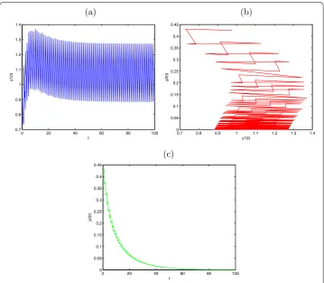
Therefore, ify() = .,y() = .,d= .,a= .,b= .,μ= .,l= .,τ= ,
D= ., then . =D>D∗= –e–aτ = .; the predator population. y
(t) will go
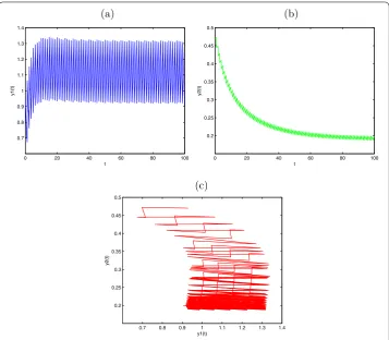
into extinction. Its dynamical behaviors can be seen in Figure . Ify() = .,y() = .,
d= .,a= .,b= .,μ= .,l= .,τ= ,D= ., then . =D<D∗= .;. the predator population are permanent. Its dynamical behaviors can be seen in Figure . Obviously, the diffusion rate between the patches affects the dynamics of System (.).
Figure 1 Globally asymptotically stabley2(t) extinction periodic solution withy1(0) = 0.5,y2(0) = 0.5, d1= 0.6,a2= 0.1,b2= 0.2,μ= 0.4,l= 0.25,τ= 1,D= 0.15. (a)Time series ofy1(t);(b)time series ofy2(t);
Figure 2 Permanence for System (3.2) withy1(0) = 0.5,y2(0) = 0.5,d1= 0.6,a2= 0.1,b2= 0.2,μ= 0.4, l= 0.25,τ= 1,D= 0.05. (a)Time series ofy1(t);(b)time series ofy2(t);(c)the phase portrait of permanence for System (3.2).
4 The dynamics Theorem . If
–e–aτ<D< (.)
and
aτ<β
d
y∗ –e–dlτ+y∗∗∗∗
e–dlτ –e–dτ (.)
hold,the prey-extinction boundary periodic solution(,y(t), )of(.)is globally asymp-totically stable,where y∗ and y∗∗∗∗ are defined as(.)and(.).
Proof First, we prove the local stability of the prey-extinction boundary periodic solution (,y(t), ) of (.). Definingx(t) =x(t),y(t) =y(t) –y(t),y(t) =y(t), then we have the following linearly similar system for (.) which concerns one periodic solution (,y(t), ):
⎛ ⎜ ⎜ ⎝
dx(t)
dt dy(t)
dt dy(t)
dt
⎞ ⎟ ⎟ ⎠=
⎛ ⎜ ⎝
a–βy(t) kβy(t) –d
a
⎞ ⎟ ⎠
⎛ ⎜ ⎝
x(t)
It is easy to obtain the fundamental solution matrix
The linearization of the fourth, fifth, and sixth equations of (.) is ⎛
The linearization of the seventh, eighth, and ninth equations of (.) is ⎛
The stability of the periodic solution (,y(t), ) is determined by the eigenvalues of
M=
According to condition (.), (.), and the Floquet theory [],i.e.
and
λ< ,
the prey-extinction boundary periodic solution (,y(t), ) of (.) is locally stable. In the following, we will prove the global attraction. From condition (.), we can choose anε> such that
ρ=exp
τ
a–β y(s) –ε
ds
< .
From the second equation of (.), we notice that dy(t)
dt ≥–dy(t). Then we consider the
following impulsive comparative differential equation:
⎧ ⎪ ⎪ ⎪ ⎪ ⎪ ⎪ ⎪ ⎪ ⎪ ⎨ ⎪ ⎪ ⎪ ⎪ ⎪ ⎪ ⎪ ⎪ ⎪ ⎩
dy(t)
dt = –dy(t), dy(t)
dt =y(t)(a–by(t)),
t= (n+l)τ,t= (n+ )τ,
y(t) =Dy(t),
y(t) = –Dy(t),
t= (n+l)τ,
y(t) =μ,
y(t) = ,
t= (n+ )τ.
(.)
From Lemma . and the comparison theorem of impulsive equations (see Theorem .. in []), we have y(t)≥y(t),y(t)≥y(t), andy(t)→y(s),y(t)→, ast→ ∞.
Then
y(t)≥y(t)≥y(s) –ε,
y(t)≥y(t)≥–ε, (.)
for alltlarge enough. For convenience, we may assume (.) holds for allt≥. From (.) and (.), we get
dx(t)
dt ≤ a–β y(s) –ε
x(t). (.)
Sox((n+ )τ)≤x(nτ+)exp[ (n+)τ
nτ (a–β(y(s) –ε))ds]. Hence,x(nτ)≤x(+)ρnand x(nτ)→ asn→ ∞, thereforex(t)→ (i= , ) ast→ ∞.
Next, we will prove thaty(t)→y(t) andy(t)→ ast→ ∞. For <ε< kdβ small enough, there must exist at> such that <x(t) <ε for allt≥t. Without loss of
generality, we may assume that <x(t) <εfor allt≥. For System (.) we have
–dy(t)≤dy(t)
dt ≤–(d–kβε)y(t), (.)
then we havey(t)≤y(t)≤y(t),y(t)≤y(t)≤y(t), andy(t)→y(t),y(t)→,
solutions of (.) and ⎧
⎪ ⎪ ⎪ ⎪ ⎪ ⎪ ⎪ ⎪ ⎪ ⎨ ⎪ ⎪ ⎪ ⎪ ⎪ ⎪ ⎪ ⎪ ⎪ ⎩
dy(t)
dt = –(d–kβε)y(t), dy(t)
dt =y(t)(a–by(t)),
t= (n+l)τ,t= (n+ )τ,
y(t) =Dy(t),
y(t) = –Dy(t),
t= (n+l)τ,
y(t) =μ,
y(t) = ,
t= (n+ )τ,
(.)
respectively. We have
y(t) =
y∗e–(d–kβε)(t–nτ), t∈[nτ, (n+l)τ),
y∗∗∗∗ e–(d–kβε)(t–(n+l)τ), t∈[(n+l)τ, (n+ )τ), (.)
wherey∗∗∗∗ =e–(d–kβε)τy∗
, andy∗is determined as
y∗= μ
–e–(d–kβε)τ.
For anyε> , there exists at,t>tsuch that
y(t) –ε<y(t) <y(t) +ε
and
y(t) –ε<y(t) <y(t) +ε.
Letε→, so we have
y(t) –ε<y(t) <y(t) +ε
and
–ε<y(t) < +ε,
fortlarge enough, which impliesy(t)→y(t) andy(t)→ ast→ ∞. This completes
the proof.
We can easily prove Theorem . similar to Theorem ..
Theorem . If
–e–a
τ+[lna+by
∗∗
(ealτ–)
a +ln
a+by∗∗∗ (eaτ–)
a+by∗∗∗ (ealτ–)]<D< –e–aτ (.)
and
aτ<β
d y
∗∗
–e–dlτ+y∗∗∗
hold, the prey-extinction boundary periodic solution (,y(t),y(t)) of (.) is globally asymptotically stable,where y∗∗ ,y∗∗∗ ,y∗∗ ,and y∗∗∗ are defined as(.)and(.).
The next task is to investigate the permanence of System (.).
Definition . System (.) is said to be permanent if there are constantsm,M> (inde-pendent of the initial value) and a finite timeTsuch that for all solutions (x(t),y(t),y(t)) with all initial values x(+) > ,y(+) > ,y(+) > ,m≤x(t)≤M,m≤y(t)≤M, m ≤ y(t) ≤ M hold for all t ≥ T. Here T may depend on the initial values
(x(+),y(+),y(+)).
Theorem . If
<D< –e–aτ (.)
and
aτ>β
d
y∗∗ –e–dlτ+y∗∗∗
e–dlτ –e–dτ (.)
hold,System(.)is permanent,where y∗∗ and y∗∗∗ are defined as(.)and(.).
Proof Suppose (x(t),y(t),y(t)) is a solution of (.) withx() > ,y() > ,y() > . By Lemma ., we have proved there exists a constantM> such thatx(t)≤M,y(t)≤M,
y(t)≤M, fortlarge enough. From (.), Theorem ., and condition (.), we have ⎧
⎪ ⎪ ⎪ ⎪ ⎨ ⎪ ⎪ ⎪ ⎪ ⎩
y(t) >y(t) –ε
>y∗∗ e–dlτ+y∗∗∗
e–d(–l)τ–ε=m, y(t) >y(t) –ε
> ay∗∗ ealτ
a+by∗∗ (ealτ–)+
ay∗∗∗ ea(–l)τ
a+by∗∗∗ (ea(–l)τ–)
–ε=m,
(.)
forεsmall enough. So we only need to findm> andεsuch thatx(t) >mfortlarge
enough. Otherwise, we can selectm> small enough satisfyingm< d
kβ, and we prove
x(t) <mcannot hold fort≥. By condition (.) and choosingε small enough, we
can obtain
σi=aτ
– β (d–kβm)
y∗∗ –e–(d–kβm)lτ+
y∗∗∗ e–(d–kβm)lτ–
e–(d–kβm)τ
–βετ
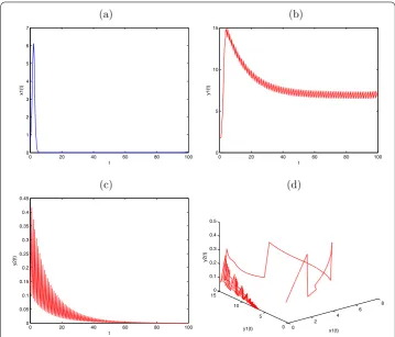
Figure 3 Globally asymptotically stable prey-extinction periodic solution (0,y1(t), 0) of System (2.1)
withx1(0) = 0.5,y1(0) = 0.5,y2(0) = 0.5,a1= 2.4,b1= 0.1,a2= 1.5,b2= 0.21,β1= 0.3,k1= 0.5,
μ= 0.86,d1= 0.1,τ= 1,l= 0.25,D= 0.78. (a)Time series ofx1(t);(b)time series ofy1(t);(c)time-series of
y2(t);(d)the phase portrait of globally asymptotically stable periodic solution (0,y1(t), 0) of System (2.1).
withy∗∗andy∗∗∗ defined as (.) and (.). Then
⎧ ⎪ ⎪ ⎪ ⎪ ⎪ ⎪ ⎪ ⎪ ⎪ ⎨ ⎪ ⎪ ⎪ ⎪ ⎪ ⎪ ⎪ ⎪ ⎪ ⎩
dy(t)
dt < –(d–kβm)y(t), dy(t)
dt =y(t)(a–by(t)),
t= (n+l)τ,t= (n+ )τ,
y(t) =Dy(t),
y(t) = –Dy(t),
t= (n+l)τ,
y(t) =μ,
y(t) = ,
t= (n+ )τ.
(.)
By Lemma ., we havey(t)≤y(t), y(t)≤y(t) andy(t)→y(t),y(t)→y(t), t→ ∞, where (y(t),y(t)) is the solution of
⎧ ⎪ ⎪ ⎪ ⎪ ⎪ ⎪ ⎪ ⎪ ⎪ ⎨ ⎪ ⎪ ⎪ ⎪ ⎪ ⎪ ⎪ ⎪ ⎪ ⎩
dy(t)
dt = –(d–kβm)y(t), dy(t)
dt =y(t)(a–by(t)),
t= (n+l)τ,t= (n+ )τ,
y(t) =Dy(t),
y(t) = –Dy(t),
t= (n+l)τ,
y(t) =μ,
y(t) = ,
t= (n+ )τ,
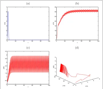
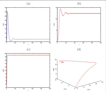
Figure 4 Globally asymptotically stable prey-extinction periodic solution (0,y1(t),y2(t)) of
System (2.1) withx1(0) = 0.5,y1(0) = 0.5,y2(0) = 0.5,a1= 2.4,b1= 0.1,a2= 1.5,b2= 0.21,β1= 0.3, k1= 0.5,μ= 0.86,d1= 0.1,τ= 1,l= 0.25,D= 0.6. (a)Time-series ofx1(t);(b)time-series ofy1(t);
(c)time-series ofy2(t);(d)the phase portrait of globally asymptotically stable periodic solution (0,y1(t),y2(t)) of System (2.1).
with ⎧ ⎪ ⎪ ⎪ ⎪ ⎪ ⎪ ⎨ ⎪ ⎪ ⎪ ⎪ ⎪ ⎪ ⎩
y(t) =
y∗∗e–(d–kβm)(t–nτ), t∈[nτ, (n+l)τ),
y∗∗∗ e–(d–kβm)(t–(n+l)τ), t∈[(n+l)τ, (n+ )τ),
y(t) = ⎧ ⎪ ⎨ ⎪ ⎩
ay∗∗ea(t–nτ)
a+by∗∗(ea(t–nτ)–)
, t∈[nτ, (n+l)τ),
ay∗∗∗ea(t–(n+l)τ)
a+by∗∗∗ (ea(t–(n+l)τ)–)
, t∈[(n+l)τ, (n+ )τ),
(.)
wherey∗∗andy∗∗are determined as ⎧
⎨ ⎩
y∗∗= B(B–a) (–A)[aC+C(B–a)]+
μ
–A> , <D< –e
–aτ,
y∗∗=B–a
C > , <D< –e
–aτ,
(.)
withA=e–(d–kβm)τ < ,B=Daealτ > ,B= ( –D)aeaτ> ,C=b(ealτ– ) > , C=b(ealτ – )[ + ( –D)ealτ] > , andy∗∗∗ andy∗∗∗ are defined as
⎧ ⎨ ⎩
y∗∗∗ =e–(d–kβm)lτy∗∗
+D×
ay∗∗ealτ
a+by∗∗(ealτ–) ,
y∗∗∗ = ( –D)× ay∗∗ealτ
a+by∗∗(ealτ–)
Figure 5 Permanence for System (2.1) withx1(0) = 0.5,y1(0) = 0.5,y2(0) = 0.5,a1= 4,b1= 0.1,a2= 4, b2= 0.21,β1= 0.3,k1= 0.1,μ= 0.01,d1= 0.1,τ= 1,l= 0.25,D= 0.01. (a)Time-series ofx1(t);
(b)time-series ofy1(t);(c)time-series ofy2(t);(d)the phase portrait of permanence for System (2.1).
Therefore, there existT> andε> such that
y(t)≤y(t)≤y(t) –ε
and
y(t)≤y(t)≤y(t) –ε.
Then
dx(t)
dt ≥ a–β
y(t) –ε
x(t), (.)
fort≥T, letN∈NandNτ>T. Integrating (.) on (nτ, (n+ )τ),n≥N, we have
x(n+ )τ≥xnτ+exp
(n+)τ
nτ
a–β
y(t) –ε
dt
=x(nτ)eσ,
thenx((N+k)τ)≥x(Nτ+)ekσ→ ∞, ask→ ∞, which is a contradiction to the
bound-edness of x(t). Hence, there exists a t > such that x(t)≥m. This completes the
Figure 6 Predator (y2(t)) extinction andx1(t) –y1(t) permanence of System (2.1) withx1(0) = 0.5, y1(0) = 0.5,y2(0) = 0.5,a1= 2,b1= 0.1,a2= 1.5,b2= 0.21,β1= 0.3,k1= 0.5,μ= 0.1,d1= 0.1,τ= 1, l= 0.25,D= 0.99. (a)Time-series ofx1(t);(b)time-series ofy1(t);(c)time-series ofy2(t);(d)the phase portrait of predator (y2(t)) extinction andx1(t) –y1(t) permanence of System (2.1).
5 Discussion
In this paper, we establish a predator-prey model with impulsive diffusion and releasing on predator population. This predator-prey model for two regions, which are connected by diffusion of the predator population, portrays the evolution of the population. We prove that all solutions of the investigated system are uniformly ultimately bounded. From Theo-rem ., the prey-extinction periodic solution (,y(t), ) of System (.) is globally asymp-totically stable. From Theorem ., the prey-extinction periodic solution (,y(t),y(t)) of
System (.) is globally asymptotically stable. From Theorem ., System (.) is perma-nent. It is assumed thatx() = .,y() = .,y() = .,a = .,b = .,a= .,
b= .,β= .,k= .,μ= .,d= .,τ= ,l= .,D= .; the conditions (.)
and (.) are obviously satisfied, then the prey-extinction periodic solution (,y(t), ) of
System (.) is globally asymptotically stable (see Figure ). It is assumed thatx() = .,
y() = .,y() = .,a= .,b= .,a= .,b= .,β= .,k= .,μ= ., d= .,τ= ,l= .,D= .; the conditions (.) and (.) are obviously satisfied, then
the prey-extinction periodic solution (,y(t),y(t)) of System (.) is globally asymptoti-cally stable (see Figure ). It is also assumed thatx() = .,y() = .,y() = .,a= ,
b= .,a= ,b= .,β= .,k= .,μ= .,d= .,τ= ,l= .,D= .; the
b= .,β= .,k= .,μ= .,d= .,τ= ,l= .,D= .; predator (y(t)) will
go into extinction andx(t) –y(t) will be permanent in System (.) (see Figure ). From the simulations, we can guess that there exist three controlling thresholds withD. It is always assumed that <D∗<D∗∗<D∗∗∗< . If <D<D∗holds, System (.) is per-manent. IfD∗<D<D∗∗holds, the prey-extinction periodic solution (,y(t),y(t)) of Sys-tem (.) is globally asymptotically stable. IfD∗∗<D<D∗∗∗holds, the prey-extinction pe-riodic solution (,y(t), ) of System (.) is globally asymptotically stable. IfD∗∗∗<D< holds, the predatory(t) will go into extinction, preyx(t) and predatory(t) will be
perma-nent. We can discuss parameterμsimilar to parameterD. We discover that the diffusive rate of the predator population plays an important role in pest management. We conclude that the impulsive diffusion and the released predator provide reliable tactic bases for pest management.
Competing interests
The authors declare that they have no competing interests.
Authors’ contributions
JJ carried out the main part of this article, LS corrected the manuscript, SH, LM, and YJ brought forward some suggestions on this article. All authors have read and approved the final manuscript.
Author details
1School of Mathematics and Statistics, Guizhou University of Finance and Economics, Guiyang, 550004, P.R. China. 2School of Continuous Education, Guizhou University of Finance and Economics, Guiyang, 550004, P.R. China.3College of
Mathematics and Information Science, Anshan Normal University, Anshan, 114007, P.R. China.
Acknowledgements
Article is supported by the National Natural Science Foundation of China (11361014, 10961008), and the project of high level creative talents in Guizhou province (No. 20164035).
Received: 27 January 2016 Accepted: 28 April 2016
References
1. Caltagirone, LE, Doutt, RL: The history of the vedalia beetle importation to California and its impact on the development of biological control. Annu. Rev. Entomol.34, 1-16 (1989)
2. DeBach, P: Biological Control of Insect Pests and Weeds. Rheinhold, New York (1964)
3. DeBach, P, Rosen, D: Biological Control by Natural Enemies, 2nd edn. Cambridge University Press, Cambridge (1991) 4. Barclay, HJ: Models for pest control using predator release, habitat management and pesticide release in
combination. J. Appl. Ecol.19, 337-348 (1982) 5. Murray, JD: Mathematical Biology. Springer, Berlin (1989)
6. Freedman, HJ: Graphical stability, enrichment, and pest control by a natural enemy. Math. Biosci.31, 207-225 (1976) 7. Grasman, J, Van Herwaarden, OA, et al.: A two-component model of host-parasitoid interactions: determination of
the size of inundative releases of parasitoids in biological pest control. Math. Biosci.169, 207-216 (2001)
8. Liu, X, Chen, L: Compex dynamics of Holling type II Lotka-Volterra predator-prey system with impulsive perturbations on the predator. Chaos Solitons Fractals16, 311-320 (2003)
9. Jiao, J, Meng, X, Chen, L: A stage-structured Holling mass defence predator-prey model with impulsive perturbations on predators. Appl. Math. Comput.189, 1448-1458 (2007)
10. Levin, SA: Dispersion and population interaction. Am. Nat.108, 207-228 (1994)
11. Allen, LJS: Persistence and extinction in single-species reaction-diffusion models. Bull. Math. Biol.45, 209-227 (1983) 12. Song, XY, Chen, LS: Uniform persistence and global attractivity for nonautonomous competitive systems with
dispersion. J. Syst. Sci. Complex.15, 307-314 (2002)
13. Cui, JA, Chen, LS: Permanence and extinction in logistic and Lotka-Volterra system with diffusion. J. Math. Anal. Appl.
258, 512-535 (2001)
14. Beretta, E, Takeuchi, Y: Global asymptotic stability of Lotka-Volterra diffusion models with continuous time delays. SIAM J. Appl. Math.48, 627-651 (1998)
15. Beretta, E, Takeuchi, Y: Global stability of single species diffusion Volterra models with continuous time delays. Bull. Math. Biol.49, 431-448 (1987)
16. Freedman, HI, Takeuchi, Y: Global stability and predator dynamics in a model of prey dispersal in a patchy environment. Nonlinear Anal.13, 993-1002 (1989)
17. Freedman, HI: Single species migration in two habitats: persistence and extinction. Math. Model.8, 778-780 (1987) 18. Freedman, HI, Rai, B, Waltman, P: Mathematical models of population interactions with dispersal ii: differential survival
in a change of habitat. J. Math. Anal. Appl.115, 140-154 (1986)
19. Freedman, HI, Takeuchi, Y: Predator survival versus extinction as a function of dispersal in a predator-prey model with patchy environment. Appl. Anal.31, 247-266 (1989)
21. Bainov, D, Simeonov, P: Impulsive Differential Equations: Periodic Solution and Applications. Longman, London (1993)
22. Jiao, J, et al.: Dynamics of a stage-structured predator-prey model with prey impulsively diffusing between two patches. Nonlinear Anal., Real World Appl.11, 2748-2756 (2010)
23. Meng, X, Chen, L: Permanence and global stability in an impulsive Lotka-VolterraN-species competitive system with both discrete delays and continuous delays. Int. J. Biomath.1, 179-196 (2008)
24. Jiao, J, et al.: An appropriate pest management SI model with biological and chemical control concern. Appl. Math. Comput.196, 285-293 (2008)
25. Jiao, J, Chen, L: Global attractivity of a stage-structure variable coefficients predator-prey system with time delay and impulsive perturbations on predators. Int. J. Biomath.1, 197-208 (2008)
26. Jiao, J, et al.: A delayed stage-structured predator-prey model with impulsive stocking on prey and continuous harvesting on predator. Appl. Math. Comput.195, 316-325 (2008)
27. Jiao, J, et al.: Analysis of a stage-structured predator-prey system with birth pulse and impulsive harvesting at different moments. Nonlinear Anal., Real World Appl.12, 2232-2244 (2011)
28. Lakshmikantham, V: Theory of Impulsive Differential Equations. World Scientific, Singapore (1989) 29. Chen, L, Meng, X, Jiao, J: Biological Dynamics. Science, Beijing (2009) (in Chinese)
30. Gakkhar, S, Negi, K: Pulse vaccination in SIRS epidemic model with non-monotonic incidence rate. Chaos Solitons Fractals35, 626-638 (2008)
31. Zhou, Y, Liu, H: Stability of periodic solutions for an SIS model with pulse vaccination. Math. Comput. Model.38, 299-308 (2003)
32. Stone, L, Shulgin, B, Agur, Z: Theoretical examination of the pulse vaccination policy in the SIR epidemic models. Math. Comput. Model.31, 207-215 (2000)
33. Gao, S, Chen, L, Nieto, JJ, Torres, A: Analysis of a delayed epidemic model with pulse vaccination and saturation incidence. Vaccine24, 6037-6045 (2006)