Cost Based Vertical Handover Decision Algorithm for WWAN/WLAN Integrated Networks

Volume 2009, Article ID 372185,11pages doi:10.1155/2009/372185

Research Article

Cost-Based Vertical Handover Decision Algorithm for

WWAN/WLAN Integrated Networks

KunHo Hong,

_{SuKyoung Lee,}

_{LaeYoung Kim,}

_{and PyungJung Song}

1_{Department of Computer Science, Yonsei University, Seoul 120-749, South Korea} 2_{LG Electronics, South Korea}

3_{Electronics and Telecommunications Research Institute (ETRI), Daejon 305-700, South Korea}

Correspondence should be addressed to SuKyoung Lee,[email protected]

Received 31 October 2008; Revised 5 March 2009; Accepted 28 May 2009

Recommended by Mohamed Hossam Ahmed

Next generation wireless communications are expected to rely on integrated networks consisting of multiple wireless technologies. Heterogeneous networks based on Wireless Local Area Networks (WLANs) and Wireless Wide Area Networks (WWANs) can combine their respective advantages on coverage and data rates, offering a high Quality of Service (QoS) to mobile users. In such environment, multi-interface terminals should seamlessly switch from one network to another in order to obtain improved performance or at least to maintain a continuous wireless connection. Therefore, network selection algorithm is important in providing better performance to the multi-interface terminals in the integrated networks. In this paper, we propose a cost-based vertical handover decision algorithm that triggers the Vertical Handover (VHO) based on a cost function for WWAN/WLAN integrated networks. For the cost function, we focus on developing an analytical model of the expected cost of WLAN for the mobile users that enter the double-coverage area while having a connection in the WWAN. Our simulation results show that the proposed scheme achieves better performance in terms of power consumption and throughput than typical approach where WLANs are always preferred whenever the WLAN access is available.

Copyright © 2009 KunHo Hong et al. This is an open access article distributed under the Creative Commons Attribution License, which permits unrestricted use, distribution, and reproduction in any medium, provided the original work is properly cited.

1. Introduction

Beyond 3G mobile networks are being defined as the

inte-gration of diverse access technologies [1,2]. One promising

way to construct integrated wireless networks is to integrate

IEEE 802.11 Wireless Local Area Networks (WLANs) [3] and

Wireless Wide Area Networks (WWANs), such as Universal Mobile Telecommunications System (UMTS) by 3rd

Gen-eration Partnership Project (3GPP) [4] and Code Division

Multiple Access 2000 (CDMA2000) by 3GPP2 [5]. These

networks have characteristics that perfectly complement each other in terms of both their data rates and coverage. Additionally, they are both widely deployed already. As a result, WWAN/WLAN-integrated networks can provide their users with a wider range of services at a higher quality. In the integrated wireless networks; a Mobile Node (MN) can

roam dynamically between different wireless networks. Thus,

one of the most important issues for integrated wireless networks is the Vertical Handover (VHO), which refers to

a handover between systems with different air interfaces.

VHOs are classified into two categories: a downward VHO (DVHO) is a handover to a wireless network with a smaller cell size and (usually) higher bandwidth per unit area; an upward VHO (UVHO) is a handover to a wireless network with a larger cell size and (usually) lower bandwidth

per unit area [6,7].

The natural trend for VHOs has been to use small-coverage, high-bandwidth networks, such as WLAN, when-ever they are available, and to remain connected to the network for as long as possible. Hence, the switch to low-bandwidth networks, such as UMTS and CDMA2000, occurs

only when a high-bandwidth network is not available [6].

This type of network selection scheme for WWAN/WLAN-integrated networks is called the WLAN-first scheme, where WLANs are always preferred by all services whenever the WLAN access is available to possibly increase bandwidth and reduce costs compared to WLANs. The studies in

[8, 9] propose the WLAN-first scheme, in which the

AP AP

AP

AP AP

BS

MN MN

MN

MN

GIF

Internet core

CN RNC

(BSC)

Network selection module

SGSN GGSN

GIF: GPRS interworking function RNC: radio network controller SGSN: serving GPRS support node GGSN: gateway GPRS support node CN: correspondent node

WWAN coverage WLAN coverage

Figure1: An overall heterogeneous networking system architecture for the proposed vertical handover decision algorithm.

The studies in [10–16] propose cost-based VHO schemes

that consider several factors, such as user preferences and network conditions, in order to perform flexible VHOs. In the cost-based VHO schemes, MN selectively changes its connection from WWAN to WLAN based on the cost function, even though the WLAN access is available. The

authors of [10] consider higher level parameters which

fall in the transport and application layers in addition

to the available access networks’ characteristics. In [11],

the handoff decision is made by the system, aiming to

achieve a better performance in the blocking

probabil-ity. The authors of [12] address the main issues that

arise while implementing the interoperability mechanisms

between two different radio access networks. Although these

VHO decision algorithms have certain advantages, they do

not consider power efficiency, which is one of the most

important aspects of wireless networks. This is especially true of integrated wireless networks since MNs with more than one wireless interface consume more power than those

with one wireless interface. The studies in [13–16] consider

the power consumption as one of the metrics for deciding VHO. However, they do not provide detailed analytical models to estimate network conditions such as available bandwidth and average user throughput in addition to power consumption.

In this paper we propose a new vertical handover decision algorithm based on a cost function for WWAN/WLAN-integrated networks. In the proposed VHO decision algo-rithm, when an MN moves from the WWAN-only area to an area that is covered by both WLAN and WWAN, DVHO is performed only if the cost of WLAN is less than that of WWAN. Our cost function considers data throughput, power consumption, and monetary cost. In addition, user preferences for these factors are considered to select an optimal network for each MN. To estimate how much throughput is obtained and how much power is drained to send and receive a bit in the target WLAN, we develop an analytical model based on Automatic Rate

Fallback (ARF) [17], which is generally used for adaptive

modulation schemes in IEEE 802.11 WLAN. Adaptive

mod-ulation schemes have been studied extensively and advocated at the physical layer in order to enhance throughput by adaptively matching transmission parameters to

time-varying wireless channel conditions [18, 19]. Therefore,

in order to benefit from the use of adaptive modulation, we assume that our VHO decision algorithm operates on IEEE 802.11 WLAN, which employs adaptive modula-tion.

The rest of this paper has the following structure. Section 2 explains the details of our proposed scheme, including an analysis of the expected available bandwidth and the expected power consumption for WLAN with

the adaptive modulation technique. Section 3 shows the

effectiveness of the proposed scheme using the results from

thorough simulations of various scenarios.Section 4presents

our conclusions.

2. Vertical Handover Decision Algorithm

2.1. Overall Architecture for the Vertical Handover Decision Algorithm. Figure 1illustrates an overall heterogeneous net-working system architecture for the proposed VHO decision

algorithm. As shown inFigure 1, our system model is based

on the generic architecture for integration of WWAN and

WLAN defined in [20]. In this architecture, the WLAN

MN enters double-coverage area?

SGSN collects information required to calculate cost from

WWAN and WLAN

Network selection module in SGSN calculates costs for both

WWAN and WLAN

Cost for WLAN<cost for WWAN

Yes No

MN performs downward VHO MN maintains the current connection with WWAN Yes

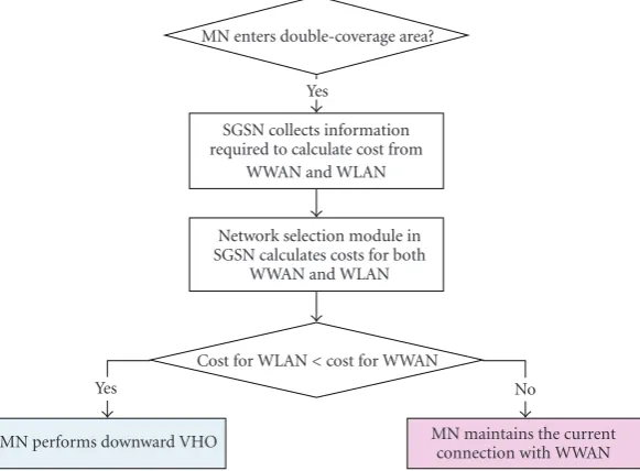
Figure2: The flow chart of the proposed vertical handover decision algorithm.

can be maintained in the system shown in Figure 1 when

the MN changes an access technology. Thus, when a VHO occurs, the packets destined to the MN can be rerouted at the SGSN by using the intra/inter-SGSN Routing Area Update

(RAU) procedure defined in [20] without going through the

reauthentication process.

We add the network selection module in SGSN to

implement the proposed VHO decision algorithm. In our

integrating architecture, thenetwork selection modulein the

SGSN not only collects all the information related to the vertical handover but also makes the decision about what network to which an MN connect-based on the results of a cost function. Therefore, GIF must provide the SGSN with information about its WLAN, which is required to calculate the cost for WLAN.

Figure 2shows the flow chart for the proposed vertical

handover decision algorithm. As shown in Figure 2, when

an MN enters the double-coverage area that is covered by both WLAN and WWAN, SGSN collects all the required information for calculating cost from both WWAN and WLAN. The collected information includes the current power consumption, data rate, and monetary cost of each bit for WWAN as well as the available modulation levels, Packet Error Rate (PER) at each modulation level, expected power consumption, and monetary cost of each bit for the target WLAN. Based on this information, SGSN calculates the cost for both networks using the proposed cost function and then decides whether the MN will perform DVHO or not. That is, if the cost for WLAN is less than that for WWAN, the MN will switch from WWAN to WLAN. The result of this decision is delivered to the MN, allowing the MN to connect to the best available network. On the other hand, UVHO is performed when the MN moves from the double-coverage area to the WWAN-only area based on RSS.

We now explain the construction of the cost function. The factors that are taken into account for our cost function

are data throughput, power consumption, and monetary

cost. The cost function for networkIis defined as

C(I)=μtft(I) +μpfp(I) +μmfm(I) forI∈ {wlan, wwan},

(1)

whereft(I), fp(I), andfm(I) denote the normalized variables

for data rate, power consumption, and monetary cost in

network I, respectively. In (1), μt, μp, and μm denote the

weights of each factor, which are set according to the user

preference. The constraint pertaining to μt, μp, and μm is

given byμt +μp+μm = 1. Note that networkI improves

with lower values ofC(I).

ft(I) is obtained as follows:

ft(I)= 1

eαtD(I)+βt, (2)

whereαt andβtare variables to adjust between ft(I), fp(I),

and fm(I) of (1). Because the three factors have different

ranges of values, each factor has adjusting variables. D(I)

is the throughput when using network I. Because the MN

uses WWAN as its current network, it knows the value

of D(wwan) by measurement. However, the MN does not

measure the value ofD(wlan) directly, and so the value is

obtained as follows:

D(wlan)=

⎧ ⎨ ⎩

B(wlan), B(wlan)< D(wwan),

ρ·B(wlan)+1−ρ·D(wwan), B(wlan)≥D(wwan),

(3)

whereB(wlan) is the expected available bandwidth of

net-work wlan. IfB(wlan) is smaller than the current throughput,

be B(wlan) because the network cannot send or receive

more thanB(wlan). If the available bandwidth is larger than

current throughput, however, then the MN can send or

receive more than D(wwan). This means that the value of

D(wlan) is between B(wlan) and D(wwan). To apply this

feature of the heterogeneous network to applications with

different bandwidth requests, we introduceρ, the value that

represents dependency between the throughput requested by

application and the network bandwidth.ρis given between

0 and 1. It is dependent on current application that is using the network. If the MN uses real-time (rt) UDP applications,

then the value is close to 0. If it uses greedy Best-Effort (BE)

TCP applications, then the value is close to 1. For example, rt UDP applications such as VoIP or video call do not need to increase network throughput, although they are connected to a high-bandwidth network. That is, such applications occupy

certain bandwidth as addressed in [21]. Thus,ρ is close to

0. If the MN has been using an rt UDP application in the WWAN-only area, that means that the WWAN admitted

the MN’s rt traffic by considering the WWAN’s load status

and checking whether the WWAN can allocate a certain

bandwidth requested by the application (i.e.,D(wwan)). If

BE TCP applications like FTP are used, however, then the throughput, that can be achieved by the applications, is

dependent on the available bandwidth [21], and soρis close

to 1. On the other hand, if the MN’ BE TCP traffic was

admitted in the WWAN with high load,D(wwan) must be

small for the MN, and hence, the throughput for the MN’s BE application may be increased by handing over to the WLAN.

The value ofB(wlan) is calculated inSection 2.2.

We now calculate the values offp(I) and fm(I). Letpw(I)

and m(I) be the power consumption and monetary cost

for a user in networkI, respectively. The expected amount

of power consumption for the target WLAN, pw(wlan),

is derived analytically in a later section, and m(I) can be

obtained by Price(I)/D(I), where Price(I) indicates the price

to transceive data in networkI per unit time. We can then

determine the normalized amount of power consumption as follows:

fp(I)= 1

eαp/ pw(I)+βp. (4)

The normalized monetary cost is defined as

fm(I)= 1

eαm/m(I)+βm. (5)

αp,βp,αm, andβm in (4) and (5) represent the adaptation

variables. Note that we take the inverse number for m(I)

andpw(I) in (4) and (5), respectively, since lower values are

better.

Whenever an MN enters the double-coverage area of WWAN and WLAN in the proposed vertical handover decision algorithm, SGSN analyzes the user preference so

thatμt,μp, andμm in (1) are set. Based on these weights as

well as the information collected from WLAN and WWAN, then SGSN calculates the costs for both WLAN and WWAN,

C(wlan) and C(wwan), respectively. The MN is allowed to

perform DVHO if the estimated cost for WLAN is less than

that for WWAN. Otherwise, the MN maintains a connection with the WWAN.

2.2. Expectation for Available Bandwidth and Power Con-sumption. In this section, we develop an analytical model to estimate the amount of power that is drained to send or receive a bit in the target WLAN. We start by establishing an analytical model of the available bandwidth for WLAN

assuming that n-level modulation is allowed. We then

estimate the amount of power consumption using this analytical model.

2.2.1. Available Bandwidth Expectation for WLAN. In order to estimate the available bandwidth for WLAN, we determine the probability that the modulation is escalated after the

transmission ofkpackets. This probability can be expressed

as a function of the probability that a packet transmission

succeeds,q, and the number of transmitted packets,k. Let

fu(k,q) be this probability. Similarly, let fd(k,p) denote

the probability that the modulation is lowered after the

transmission of packetk, where p is the probability that a

packet transmission fails, that is, packet error rate (PER). For analysis, we assume that the wireless channel is a Gaussian channel, in which each bit has the same bit error probability, and bit errors are identically and independently distributed

over the whole frame as in [22].

LetNbe the number of successfully transmitted packets

that is required to elevate the modulation level, and letK

be the number of unsuccessfully transmitted packets that is required to degrade the modulation level. That is, the next higher modulation level is selected after transmitting

consec-utiveNframes successfully while the next lower modulation

level is selected after failing to transmit consecutiveKframes.

Depending on the value ofk, fu(k,q) can be decomposed

into four cases as follows.

(1) Whenk < N. The modulation remains unchanged

since consecutive N packets are not successfully

transmitted, resulting infu(k,q)=0.

(2) When k = N. All N packets in the transmission

should succeed so thatfu(k,q) is computed asqN_.

(3) When k = N + 1. In this case, the first packet

transmission should fail, followed byN consecutive

successful packets, resulting inpqN_.

(4) Whenk > N+ 1. As shown inFigure 3, we can divide

this case into two components. In the first com-ponent, the modulation should remain unchanged

during the transmission of the firstk−N−1 packets.

Let Au(k − N − 1,q) be this probability. In the

second component, the (k−N)th packet transmission

should fail, followed by the successful transmission

of N consecutive packets, resulting in pqN_{. Thus,}

fu(k,q)=Au(k−N−1,q)pqN_{is the joint probability.}

Note that the (k−N)th packet failure is necessary.

Otherwise, the modulation can be elevated after the

Failed packet Successful packet

N

Receiver 1 2 . . . k−N−1 k−N k−N+ 1 . . . k Sender

1st component 2nd component

Figure3: The case that the modulation is elevated after the transmission ofkpackets whenk > N+ 1.

A failed packet before successive N packets

the complement probabilities from 1 instead of calculating them directly. The complement events, which mean that the modulation is changed during the transmission of the first

k−N−1 packets, consist of the three cases shown inFigure 4.

Case 1. The modulation can be elevated during the

trans-mission of the firstk−N−1 packets. This probability can be

recursively computed by k_m−₌N₁−1 fu(m,q).

Case 2. In contrast with Case 1, the modulation can be

lowered before the (k − N)th packet, though it is still

computed by mk−=N1−1fd(m,p), as in Case1.

Case 3. It is also possible that the modulation remains

unchanged after transmittingk−N−1 packets, but after

sending theK −Nth packet, the modulation degrades. In

this case, the failure ofK sequential packets occurs after the

first phase, as shown inFigure 4. It is not included in Cases1

and2.fd(k−N,p) is the probability that modulation falls at

k−Nth packet. However, the last packet, ork−Nth packet, is

not included in the first phase, and so the probability of this

case is (1/ p)fd(k−N,p).

By summing up all of the above three cases, we have Au(k−N −1,q) = 1− k−N−1

m=1 {fu(m,q) + fd(m,p)} −

(1/ p)fd(k−N,p).

Using the opposite derivation process, we can also obtain

fd(k,p) as follows:

of packets until the modulation is altered when the current

modulation is given. Letgu(q) andgd(p) denote the average

numbers of packets until the modulation is escalated and

lowered, respectively. Along with fu(k,q) and fd(k,p), we

A key observation found in the ARF algorithm is that the transmission rate is always switched to adjacent one, so that the rate adaptation procedure of ARF could be expressed via

a birth-death Markov chain as in [23]. Figure 5shows the

Markov chain where the statei represents the modulation

leveliof the single target station. Then, we can model then

-level modulation technique as a simple queueing system with

the state of the modulation level as shown inFigure 5, where

λi andμi denote the rates that the modulation is elevated

Modulation

Figure5: The queueing system with the state of modulation level.

λi andμi can then be expressed as functions ofgu(qi) and

gd(pi), respectively:

λi=

whereqiand pirepresent the success and failure

probabili-ties, respectively, when the modulationMiis used.

From (9) and (10), the steady-state probability that the

modulation leveliis used, f(i), can be derived as

We assume thatBiandpiare the maximum bandwidths

provided by the target WLAN and the PER at the modulation

level i, respectively. Finally, we obtain Bwlan, the expected

bandwidth of the WLAN, as follows:

Bwlan=

Letθwlanbe the current usage of the WLAN.θwlanis defined

as the fraction of time during which the AP finds that the channel is busy for unit time: it can be obtained by the AP of

the WLAN as in [21]. Then, we obtain the expected available

bandwidth of the WLAN,B(wlan), as follows:

Bwlan=(1−θwlan)·Bwlan. (13)

2.2.2. Estimation of Power Consumption. In this section we estimate the amount of power consumption for both WLAN

and WWAN. Let Din and Dout denote the receiving and

sending bit rates in WWAN, respectively. We then obtain the average amount of power consumption required to send or

receive a single bit in WWAN,pw(wwan), by measuring the

average amount of power consumption per unit time,δwwan,

as follows:

pw(wwan)= δwwan

(Din+Dout). (14)

As done in WWAN, we denote the receiving and sending

bit rates in WLAN by Din and Dout. Let δwlanr , δwlant , and

δwlani denote the amount of power consumed per unit

time to receive, send, and stay-in-idle mode in WLAN, respectively. We can then obtain the average amount of power consumption in WLAN as follows:

pw(wlan)

whereBwlan is the available effective bandwidth for WLAN

and can be obtained as derived inSection 2.2.1.

Here we assume that the bit rate in WLAN is affected

by the difference in overall network bandwidth between

WLAN and WWAN as well as the characteristic of ongoing

applications. The amount of data throughput in WLAN,D,

is then computed as

D=Din +Dout =(Din+Dout)

where ρ represents the implementation variable based on

the characteristic of application, as mentioned earlier (0 ≤

ρ ≤ 1). Assuming that Din and Dout are adapted to the

increased/decreased bandwidth with the same ratio, our pro-posed scheme estimates a reduction in power consumption

by using (14), as well as (15), if the MN performs DVHO.

3. Performance Evaluation via Simulation

We have developed the simulator using C++ to investigate

the effectiveness of our proposed scheme in comparison

with that of the existing WLAN-First Scheme (WFS) and

a cost-based scheme [14] where a cost function of power

consumption, available bandwidth, and monetary cost, is used for network selection. The proposed scheme takes account of the MN’s RSS and ARF when computing the cost for each network, whereas the cost-based scheme does not. Our simulation model accounts for the throughput and power consumption as performance metrics. The number of VHOs is also evaluated.

3.1. Simulation Environment. In our simulation, we use the

network topology illustrated inFigure 1 in which five APs

are deployed in a single WWAN coverage of 500×500 m2_.

As shown in Figure 1, each AP in the network topology

covers a circular area with a radius of 100 m and employs

IEEE 802.11a standard protocol [24], including an adaptive

Table1: The characteristics of modulation for 802.11A.

Modulation

level (i) 1 2 3 4 5

Bandwidth (Bi)

6 Mbps 12 Mbps 18 Mbps 36 Mbps 54 Mbps

Modulation BPSK QPSK QPSK 16-QAM 64-QAM

Coding Rate 1/2 1/2 3/4 3/4 3/4

ai 274.7229 90.2514 67.6181 53.3987 35.3508

gi 7.9932 3.4998 1.6883 0.3956 0.0900

γpi(dB) −1.5331 1.0942 3.9722 10.2488 15.9784

In our simulation, the bandwidth for WLAN is set to a maximum of 54 Mbps, while the WWAN uses the bandwidth of High-Speed Downlink Packet Access (HSDPA), 14 Mbps. The data rate for WLAN changes adaptively based on an adaptive modulation technique through which five

modu-lation levels are available. Table 1 shows the characteristics

of the five modulation levels for 802.11a adopted in our

simulation [19,24]. BothKandNfor adaptive modulation

are set to 10.

In our simulation, the PER at each modulation levelifor

WLAN is modeled in [19, Equation (5)] as follows:

piγ≈

⎧ ⎨ ⎩

1, if 0< γ < γpi

aie−giγ_{, ifγ}≥_γpi,

(17)

whereγrepresents the received signal-to-noise ratio (SNR).

The level-dependent parametersai,gi, andγpi are obtained

by fitting (17) to the exact PER. Supposing that a packet

length is 1080 bits, thenTable 1provides the fitting

param-eters for transmission modes. Assuming that the path-loss

exponent is 3, the received SNR,γ, is computed as follows

[18]:

γ=Pt−PL(d0)−30 log₁₀d+G(t), (18)

where Pt is the transmit power, PL(d0) = 46.7 dB is the

mean path loss at a close reference distance ofd0=1 m,dis

the distance in meters, andG(t) is a time-variant

Rayleigh-distributed fading gain, for which the well-known Jakes’ Doppler spectrum is assumed.

The Correspondent Node (CN) generates two different

classes of traffic: BE TCP traffic (ρ = 1) and UDP traffic

(ρ = 0). The data session arrival rate follows a Poisson

process with mean 1/300. The packet size is 1000 bytes. In the simulation, TCP Reno has been implemented, where the initial and maximum window sizes are set to 1 and 1024 packets, respectively. Each session generates a file with the size varying from 1 to 11 Mbytes. To simulate the

UDP traffic, On/Off traffic is generated, where the On

and Off periods are exponentially distributed with means

of 100 seconds and 300 seconds, respectively. During On

period, traffic is generated with a rate of 20 to 200 Kbytes/s.

We obtain the values of (αt,βt), (αp,βp), and (αm,βm)

in (2), (4), and (5) from the simulation such that they

normalize the value of each factor, that is, ft(I), fp(I), and

fm(I). Table 2 gives these values. In our simulation, the

Table2: Adaptation variables for each factor.

αt 0.003 βt 0

αp 0.6 βp 0

αm 2 βm 0

Table3: Parameter values for mobility model.

Parameter Input 1 Input 2

vmax 0.66 m/s 1.54 m/s

amin −0.18 m/s2 −0.42 m/s2

amax 0.12 m/s2 0.28 m/s2

Tv 125 s

Tϕnew 600 s

amounts of power consumed to transmit, receive, and stay in an idle state are set to 1.828 W, 1.0494 W, and 0.6699 W, respectively, for the WLAN interface. These amounts are set to 2.805 W, 0.495 W, and 0.066 W, respectively, for the WWAN interface. The ratio of Price(wwan) and Price(wlan) is set to 5 to 1. The simulation time in the simulator is 100 hours.

For the mobility of MNs, we use the Smooth Random Mobility model, in which there is a maximum speed,

vmaxm/s, and a set of two preferred speeds,vpre f1=(3/5)vmax

and vpre f2 = vmax [25]. In our simulation, a total of six

MNs move at pedestrian speeds. The initial velocity of each

MN is chosen from the two preferred speeds,vpre f1,vpre f2,

and the range [0,vmax] with probabilities of 0.2, 0.5, and

0.3, respectively. We assume a uniform distribution on the

range of [0,vmax]. All the MNs move with the selected

speed until a new target speed is set again. The target speed is updated at every time interval which follows an

exponential distribution with a mean of Tvs. Whenever

a new target speed is decided, the MN decelerates or accelerates until the target speed is reached or a new target

speed is decided again.aminandamax denote the maximum

possible deceleration and acceleration in m/s2_{, respectively.}

The MN selects a random acceleration/deceleration value

from [amin, amax]. It also decides whether to change its

movement direction or to maintain it with probabilities of

1/6 and 5/6, respectively. This is done at every time interval

with an exponential distribution, the mean of which is Tϕnews.

All the parameter values for the mobility model are

obtained from [25, 26] and are given in Table 3. In the

simulation, MNs move in accordance with two input sets that

represent two different levels of mobility, as shown inTable 3.

That is, half of the MNs move according to Input 1, and the other half of the MNs move according to Input 2.

3.2. Simulation Results. We first run simulation tests by

setting the weights (μm,μt,μp) in (1), which represent user

preference, all to 1/3 for the proposed scheme. To determine

the impact of the weights in (1) on the performance of

0

Figure6: File size per session versus throughput when the TCP traffic (ρ=1) is generated.

different combinations ofμm,μt, andμp. We run simulation

tests for the proposed scheme with another three weight sets that make the data throughput, the power consumption, and the monetary cost most important, respectively, among the three factors in our cost function. The three weight sets are

(μm,μt,μp)=(0.8, 0.1, 0.1), (0.1, 0.8, 0.1), and (0.1, 0.1, 0.8).

The values for performance metrics in simulation results are those averaged over all the MNs.

Figure 6shows the throughput performance for different

file sizes when the TCP traffic (ρ = 1) is generated. We

observe fromFigure 6that both the proposed and the

cost-based schemes achieve much better throughput performance than WFS over the whole range of the file size. Specifically, the throughput improvement by our scheme over WFS is

17.3% in average.Table 4(a) shows the relative throughput

performance gains of our scheme with the four weight sets

and the cost-based scheme over WFS when ρ is 1. We

see that when a higher weight is put on the throughput

(i.e.,μt = 0.8), our scheme shows the highest throughput

improvement. It can be also seen from Table 4(a) that the

throughput is also improved by the proposed scheme over the cost-based scheme.

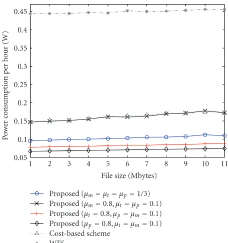
Figure 7shows the power consumption per minute in

Watts versus the different file sizes when the TCP traffic (ρ=

1) is generated. We see fromFigure 7that both the proposed

and the cost-based schemes show less power consumption than WFS for all the values of the file size. It is also observed fromFigure 7that our scheme consumes less power than the

cost-based scheme except for the case ofμm =0.8, in which

the power consumption for the proposed scheme is almost same as that for the cost-based scheme since 80% of the weight is put on the monetary cost in the proposed scheme.

0.05

Figure7: File size per session rate versus power consumption per minute when the TCP traffic (ρ=1) is generated.

Specifically,Table 4(b) shows the relative performance gains

of our scheme with the four weight sets and the cost based scheme over WFS in terms of the power consumption when

ρ is 1. As expected, the proposed scheme with μp = 0.8

shows the most performance gain. Our scheme decreases the power consumption per minute from those of WFS and the cost-based scheme by 76.71% and 35.35%, respectively, in average.

Figure 8 shows the number of VHOs per hour for the

different file sizes when the TCP traffic (ρ=1) is generated.

We see that the WFS yields a larger number of VHOs, compared to both the proposed and the cost-based schemes. In the proposed scheme, the average number of VHOs performed by each MN is 85.51% less than that of WFS in average. This is because WFS lets each MN perform DVHO whenever the MN enters the double-coverage area. The cost-based scheme shows almost the same number of VHOs as

the proposed scheme with μm = 0.8, whereas our scheme

performs 73.7% less VHOs than the cost-based scheme, in average.

From Figures6,7, and8, we can see that when the TCP

traffic is generated, our scheme outperforms WFS in terms of

the throughput and the power consumption for the different

file sizes, while yielding a smaller number of VHOs than WFS. It can be also seen that the proposed scheme achieves better performance than the cost-based scheme in terms of the throughput, the power consumption, and the number of VHOs, except for the case in which 80% of weight is put on the monetary cost.

We now evaluate the performance of our VHO decision

algorithm when the UDP traffic (ρ = 0) is generated.

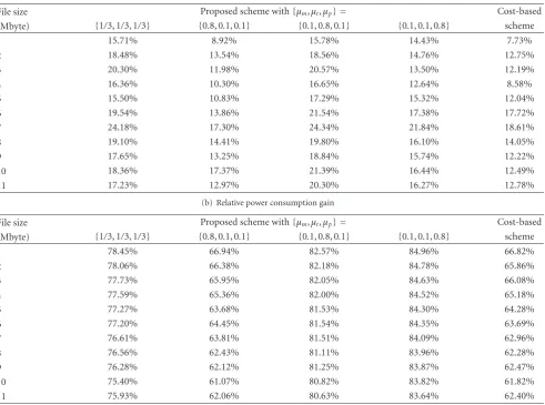
Table4: Relative performance gain of the proposed and the cost-based schemes over WFS when the TCP traffic (ρ=1) is generated.

(a) Relative throughput gain

File size Proposed scheme with{μm,μt,μp} = Cost-based

(Mbyte) {1/3, 1/3, 1/3} {0.8, 0.1, 0.1} {0.1, 0.8, 0.1} {0.1, 0.1, 0.8} scheme

1 15.71% 8.92% 15.78% 14.43% 7.73%

2 18.48% 13.54% 18.56% 14.76% 12.75%

3 20.30% 11.98% 20.57% 13.50% 12.19%

4 16.36% 10.30% 16.65% 12.64% 8.58%

5 15.50% 10.83% 17.29% 15.32% 12.04%

6 19.54% 13.86% 21.54% 17.38% 17.72%

7 24.18% 17.30% 24.34% 21.84% 18.61%

8 19.10% 14.41% 19.80% 16.10% 14.05%

9 17.65% 13.25% 18.84% 15.74% 12.22%

10 18.36% 17.37% 21.39% 16.44% 12.49%

11 17.23% 12.97% 20.30% 16.27% 12.78%

(b) Relative power consumption gain

File size Proposed scheme with{μm,μt,μp} = Cost-based

(Mbyte) {1/3, 1/3, 1/3} {0.8, 0.1, 0.1} {0.1, 0.8, 0.1} {0.1, 0.1, 0.8} scheme

1 78.45% 66.94% 82.57% 84.96% 66.82%

2 78.06% 66.38% 82.18% 84.78% 65.86%

3 77.73% 65.95% 82.05% 84.63% 66.08%

4 77.59% 65.36% 82.00% 84.52% 65.18%

5 77.27% 63.68% 81.53% 84.30% 64.28%

6 77.20% 64.45% 81.54% 84.35% 63.69%

7 76.61% 63.81% 81.51% 84.09% 62.96%

8 76.56% 62.43% 81.11% 83.96% 62.28%

9 76.28% 62.12% 81.25% 83.87% 62.47%

10 75.40% 61.07% 80.82% 83.82% 61.82%

11 75.93% 62.06% 80.63% 83.64% 62.40%

Table5: Data transmission rate (Kbyte/s) versus throughput when the UDP traffic (ρ=0) is generated.

Data transmission Proposed scheme with{μt,μp,μm} = WFS Cost-based

Rate (Kbytes/s) {1/3, 1/3, 1/3} {0.8, 0.1, 0.1} {0.1, 0.8, 0.1} {0.1, 0.1, 0.8} scheme

20 4.67 4.67 4.96 4.57 4.64 4.50

40 9.39 9.19 10.01 9.28 9.14 9.16

60 14.37 13.97 14.84 13.82 13.80 13.73

80 18.46 18.64 19.56 18.53 18.35 18.52

100 23.45 23.53 25.04 22.96 22.48 22.89

120 28.18 27.80 30.39 27.70 27.17 27.66

140 32.95 32.92 35.18 32.12 32.06 32.36

160 37.07 37.91 39.00 36.52 37.36 37.83

180 42.52 42.12 45.11 40.65 41.47 41.55

200 44.84 45.97 49.89 45.57 45.63 45.12

220 51.98 51.54 55.86 50.73 50.43 51.16

values of the data transmission rate when ρ = 0. We run

simulation tests for the proposed scheme with the four weight sets, as in the simulation for the TCP. We observe fromTable 5that the proposed and the cost-based schemes and WFS have similar throughput performances, because

when ρ is 0, the amount of data throughput achieved by

WWAN is same as that achieved by WLAN, as known from

(16).

Figure 9depicts the power consumption per minute for

0

Figure8: File size per session versus number of VHOs per hour when the TCP traffic (ρ=1) is generated. Data transmission rate (Kbytes/s)

Proposed (μm=μt=μp=1/3)

Figure9: Data transmission rate versus power consumption per minute when the UDP traffic (ρ=0) is generated.

UDP traffic (ρ = 0) is generated. We see from Figure 9

that our scheme with μp = 0.8 achieves the greatest

improvement over the WFS and the cost-based scheme in terms of the power consumption. Specifically, our scheme

with μp = 0.8 decreases the power consumption per

minute 83.71% and 68.35% from those of WFS and the

0 Data transmission rate (Kbytes/s)

Proposed (μm=μt=μp=1/3)

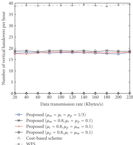
Figure10: Data transmission rate versus number of VHOs per hour when the UDP traffic (ρ=0) is generated.

cost-based scheme, respectively, in average. For the other

three weigh sets (i.e., μt = 0.8, μm = 0.8, and all the

weights are 1/3), our scheme consumes 1.33% less power than the cost-based scheme in average, because less weight

is put on the power cost, compared to the case of μp =

0.8.

Figure 10shows the number of VHOs per hour for the

different values of the data transmission rate when the UDP

traffic (ρ =0) is generated. We see that WFS, in which the

MN performs DVHO whenever it enters the double-coverage area, shows the greatest number of VHOs. The number of VHOs for the cost-based scheme is 2.8% more than our

scheme with the three weight sets (excludingμp = 0.8), in

average. However, for our scheme withμp=0.8, no VHO is

performed over the whole range of the data transmission rate in order to comply with the user’s request and to save power as much as possible.

4. Conclusion

The coexistence of different wireless access technologies

scheme, when an MN moves to the double coverage area, DVHO is performed only if the cost expected in the WLAN is less than that in the WWAN. The cost function is based on data throughput, power consumption, and monetary cost. In addition, user preferences for these cost factors are considered to select an optimal network for each MN. Our simulation results showed that the proposed scheme outperforms the typical WFS scheme in terms of throughput and power consumption by selecting a lower cost network over all user preferences.

Acknowledgments

This work was supported in part by the IT R&D program of MKE/IITA (2009-F-043-01, Development of user-centric terminal-controlled seamless mobility technology) and in part by the Information Technology Research Center (ITRC) support program supervised by the MKE/IITA, South Korea (IITA-2009-C1090-0902-0005).

References

[1] N. Nasser, A. Hasswa, and H. Hassanein, “Handoffs in fourth generation heterogeneous networks,” IEEE Communications Magazine, vol. 44, no. 10, pp. 96–103, 2006.

[2] Y. Kim, B. J. Jeong, J. Chung, et al., “Beyond 3G: vision, requirements, and enabling technologies,”IEEE Communica-tions Magazine, vol. 41, no. 3, pp. 120–124, 2003.

[3] IEEE 802.11, “Wireless LAN Medium Access Control (MAC) and Physical Layer (PHY) Specifications,” IEEE Standard, 1999.

[4] 3GPP TR 23.234 v7.7.0, “3GPP System to WLAN Inter-working; System Description (Release 7),” March 2008,

http://www.3gpp.org/Specifications.

[5] 3GPP2, “CDMA2000 WLAN Interworking,” S.R0087-A, v1.0, March 2006,http://www.3gpp2.org.

[6] K. Pahlavan, P. Krishnamurthy, A. Hatami, et al., “Handoffin hybrid mobile data networks,”IEEE Personal Communications, vol. 7, no. 2, pp. 34–47, 2000.

[7] M. Lott, M. Siebert, S. Bonjour, D. von Hugo, and M. Weckerle, “Interworking of WLAN and 3G systems,” IEE Proceedings: Communications, vol. 151, no. 5, pp. 507–513, 2004.

[8] M. Ylianttila, R. Pichna, J. Vallstrom, et al., “Handoff pro-cedure for heterogeneous wireless networks,” inProceedings of the IEEE Global Telecommunications Conference (GLOBE-COM ’99), vol. 5, pp. 2783–2787, December 1999.

[9] Q. Zhang, C. Guo, Z. Guo, and W. Zhu, “Efficient mobil-ity management for vertical handoff between WWAN and WLAN,”IEEE Communications Magazine, vol. 41, no. 11, pp. 102–108, 2003.

[10] A. Calvagna and G. Modica, “A cost-based approach to vertical handover policies between WiFi and GPRS,”Wireless Communications and Mobile Computing, vol. 5, no. 6, pp. 603– 617, 2005.

[11] W. Shen and Q.-A. Zeng, “A novel decision strategy of vertical handoffin overlay wireless networks,” in Proceedings of the 5th IEEE International Symposium on Network Computing and Applications (NCA ’06), pp. 227–230, 2006.

[12] T. Al-Gizawi, K. Peppas, D. I. Axiotis, E. N. Protonotarios, and F. Lazarakis, “Interoperability criteria, mechanisms, and eval-uation of system performance for transparently interoperating WLAN and UMTS-HSDPA networks,”IEEE Network, vol. 19, no. 4, pp. 66–72, 2005.

[13] J. McNair and F. Zhu, “Vertical handoffs in fourth-generation multinetwork environments,”IEEE Wireless Communications, vol. 11, no. 3, pp. 8–15, 2004.

[14] L.-J. Chen, T. Sun, B. Chen, V. Rajendran, and M. Gerla, “A smart decision model for vertical handoff,” inProceedings of the ANWIRE International Workshop on Wireless Internet and Reconfigurability, 2004.

[15] Q. Song and A. Jamalipour, “A time-adaptive vertical handoff decision scheme in wireless overlay networks,” inProceedings of the IEEE International Symposium on Personal, Indoor and Mobile Radio Communications (PIMRC ’06), 2006.

[16] R. Tawil, G. Pujolle, and O. Salazar, “A vertical handoff deci-sion scheme in heterogeneous wireless systems,” inProceedings of the IEEE Vehicular Technology Conference, pp. 2626–2630, 2008.

[17] A. Kamerman and L. Monteban, “WaveLAN-II: a high-performance wireless LAN for the unlicensed band,”Bell Labs Technical Journal, vol. 2, no. 3, pp. 118–133, 1997.

[18] P. Chevillat, J. Jelitto, A. N. Barreto, and H. L. Truong, “A dynamic link adaptation algorithm for IEEE 802.11a Wireless LANs,” inIEEE International Conference on Communications (ICC ’03), vol. 2, pp. 1141–1145, 2003.

[19] Q. Liu, S. Zhou, and G. B. Giannakis, “Cross-layer combining of adaptive modulation and coding with truncated ARQ over wireless links,”IEEE Transactions on Wireless Communications, vol. 3, no. 5, pp. 1746–1755, 2004.

[20] 3GPP, “General Packet Radio Service(GPRS); Service Descrip-tion Stage 2 (Release 7),” Technical SpecificaDescrip-tions 3GPP TS 23.060 v7.4.0, March 2007.

[21] H. Zhai, J. Wang, and Y. Fang, “Providing statistical QoS guarantee for voice over IP in the IEEE 802.11 wireless LANs,” IEEE Wireless Communications, vol. 13, no. 1, pp. 36–43, 2006. [22] Q. Ni, T. Li, T. Turletti, and Y. Xiao, “Saturation throughput analysis of error-prone 802.11 wireless networks,” Wireless Communications and Mobile Computing, vol. 5, no. 8, pp. 945– 956, 2005.

[23] Q. Pang, V. C. M. Leung, and S. C. Liew, “A rate adaptation algorithm for IEEE 802.11 WLANs based on MAC-layer loss differentiation,” in Proceedings of the 2nd International Conference on Broadband Networks (BroadNets ’05), pp. 709– 717, October 2005.

[24] IEEE 802.11a, “Wireless LAN Medium Access Control (MAC) and Physical Layer (PHY) Specifications: High-speed Physical Layer in the 5 GHz Band,” IEEE Standard, 1999.

[25] C. Bettstetter, “Smooth is better than sharp: a random mobil-ity model for simulation of wireless networks,” inProceedings of the 4th ACM International Workshop on Modeling, Analysis and Simulation of Wireless and Mobile Systems (MSWiM ’01), pp. 19–27, July 2001.