R E S E A R C H
Open Access
Numerical algorithm for nonlinear
delayed differential systems of
n
th order
Josef Rebenda
1*and Zden ˇek Šmarda
2*Correspondence:
[email protected] 1CEITEC BUT, Brno University of Technology, Brno, Czech Republic Full list of author information is available at the end of the article
Abstract
The purpose of this paper is to propose a semi-analytical technique convenient for numerical approximation of solutions of the initial value problem forp-dimensional delayed and neutral differential systems with constant, proportional and time varying delays. The algorithm is based on combination of the method of steps and the differential transformation. Convergence analysis of the presented method is given as well. Applicability of the presented approach is demonstrated in two examples. A system of pantograph type differential equations and a system of neutral functional differential equations with three types of delays are considered. The accuracy of the results is compared to those obtained by the Laplace decomposition algorithm, the residual power series method and Matlab package DDENSD. A comparison of computing time is presented, too, showing reliability and efficiency of the proposed technique.
MSC: 34K28; 34K07; 34K40; 65L03
Keywords: Differential transformation; Method of steps; Delayed differential system; Multiple delays
1 Introduction
Systems of functional differential equations (FDEs), in particular delayed or neutral differ-ential equations, are often used to model processes in the real world. To give some exam-ples, we mention models in population dynamics [1], neuromechanics [2], machine tool vibrations [3], etc. Further models and details can be found, for instance, in monographs [4] and [5].
Semi-analytical methods expressing solutions to problems with delays in a series form have been studied in the last two decades. Methods such as the variational iteration method (VIM) [6], Adomian decomposition method (ADM) [7], homotopy perturbation method (HPM) [8], homotopy analysis method (HAM) [9] and also methods based on the Taylor theorem such as the differential transformation (DT) [10], Taylor collocation method [11] and Taylor polynomial method [12] have been developed to approximate so-lutions to different problems for FDEs. Other ways to use the series approach in solving FDEs are, e.g., the method of polynomial quasisolutions [13,14], finite difference methods [15,16], and the functional analytic technique (FAT) [17,18].
The main aim of the work is to apply a combination of the method of steps and DT as a convenient tool for finding an approximate solution to the initial value problem for
functional differential systems used in dynamical models. Convergence analysis and er-ror estimates of the method are investigated as well. We give some experimental results in Sect.4to show that the algorithm produces reliable results with the same or better efficiency than the reference methods.
2 Methods
The main idea of our approach is to combine the differential transformation and general method of steps.
The differential transformation has been, and still is, an active research topic during the last years. As examples of recently published results, we mention research papers [19–23]. These papers among other publications contain new algorithms and their applications to solving different problems involving differential equations.
Definition 1 The differential transformation of a real functionu(t) at a pointt0∈Ris
D{u(t)}[t0] ={U(k)[t0]}∞k=0, where thekth componentU(k)[t0] of the differential
transfor-mation of the functionu(t) att0is defined as
U(k)[t0] =
1 k!
dku(t) dtk
t=t0
, (1)
assuming that the original functionu(t) is analytic.
Definition 2 The inverse differential transformation of{U(k)[t0]}∞k=0att0is defined as
u(t) =D–1U(k)[t0]
∞
k=0
[t0] =
∞
k=0
U(k)[t0](t–t0)k. (2)
In applications, the functionu(t) is usually expressed in the form of finite series
u(t) = N
k=0
U(k)[t0](t–t0)k. (3)
In Sect.4, we use the following transformation formulas, which are derived from defini-tions (1), (2) and proved in [24].
Lemma 1 Assume that W(k),U(k)and Ui(k)are the kth components of the differential transformations of functions w(t),u(t)and ui(t), i= 1, 2,at t0∈R,respectively,and let
q,qj∈(0, 1),j= 1, 2.Moreover,assume that t0= 0.DenoteN0=N∪ {0}.
If w(t) =d nu(t)
dtn , then W(k) = (k+n)!
k! U(k+n).
If w(t) =u1(t)u2(t), then W(k) =
k
l=0
U1(l)U2(k–l).
If w(t) =u(qt), then W(k) =qkU(k).
If w(t) =u1(q1t)u2(q2t), then W(k) =
k
l=0
If w(t) =d
Remark1 Transformation formulas for shifted argumentsw(t) =u(t–a) are often proved and applied in papers. However, using these formulas when solving initial value problems for delayed differential equations is not convenient since the uniqueness of solutions is violated. The reason is that the values of the initial vector function fort< 0 are not taken into account.
One of the drawbacks of the common approach to the differential transformation is that there is no use of direct transformation formulas for equations with nonlinear terms containing unknown functionu(t), for instance,f(u) =ecosuorf(u) =√1 +u4.
Fortunately, the corresponding transformations can be calculated using the Adomian polynomialsAn, in which each solutionuiis replaced by the corresponding components Ui(k) of the differential transformation{Ui(k)}k∞=0, see [25]. Suppose thatF(k) is thekth component of the differential transformation of a nonlinear termf(u), then
F(k) =
Recently, it turned out that there is another way to work with nonlinearities in DT [26]. The second method, namely the method of steps, enables us to replace the terms in-volving constant or time-dependent delays by the initial vector function and its deriva-tives. Then the original initial value problem for a system of delayed or neutral differential equations is simplified to the initial problem for a system of ordinary differential equa-tions. Details on the method of steps can be found, e.g., in monographs [4,5,27].
3 Results
u(mi)(αi(t))) are (m
i·p)-dimensional vector functions,mi≤n,i= 1, 2, . . . ,r, r∈Nand fj: [0,∞)×Rnp×Rωpare continuous real functions forj= 1, 2, . . . ,p, whereω=
r i=1mi.
We consider three types of delaysαi:
1. αi(t) =qit, whereqi∈(0, 1)(proportional delay).
2. αi(t) =t–τi, whereτi> 0is a real constant (constant delay).
3. αi(t) =t–τi(t), whereτi(t)≥τi0> 0fort> 0is a real function (time-dependent or
time-varying delay).
Lett∗=min1≤i≤r{inft>0(αi(t))} ≤0,m=max{m1,m2, . . . ,mr} ≤n. In the casem=n, sys-tem (5) is a neutral system, otherwise it is a delayed differential system.
Ift∗< 0, an initial vector functionΦ(t) = (φ1(t), . . . ,φp(t))Tmust be assigned to system (5) on the interval [t∗, 0]. Moreover, we assume thatφj(t)∈Cn([t∗, 0],R) forj= 1, . . . ,p.
We look for a solution of system (5) with the following initial conditions:
u(0) = v0, u(0) = v1, . . . , u(n–1)(0) = vn–1, (6)
and the initial vector functionΦ(t) on interval [t∗, 0] satisfying
Φ(0) = u(0), . . . , Φ(n–1)(0) = u(n–1)(0). (7)
We solve initial value problem (5), (6) and (7) subject to the following hypotheses: (H1) The functionsfj,j= 1, . . . ,pare analytic in[0,T∗]×Rnp×Rωp.
(H2) The initial value problem (5), (6) and (7) has a unique solution on some interval [0,T∗].
Remark2 Hypothesis (H2) is valid, for example, if the delay functionsαiare Lipschitz continuous on [0,T∗], the functionsφj,φj, . . . ,φ(jn)are Lipschitz continuous on [t∗, 0], and the functionsfjare continuous with respect toton [0,T∗] and Lipschitz continuous with respect to the rest of the variables onRnp×Rωp. More details and other types of sufficient conditions for existence of a unique solution can be found in [5, Sects. 3.2 and 3.3], or [27, Sect. 2.2].
We start with the method of steps. We substitute the initial vector functionΦ(t) and its derivatives in all places where the unknown functions with constant or time-dependent delays and derivatives of those functions take place. This turns the delayed system (5) into a system of ordinary differential equations or differential equations with proportional delays in the case when system (5) contains proportional delays.
For example, ifα1(t) =t–τ1,α2(t) =t–τ2,α3(t) =q3tandα4(t) =t–τ4(t), applying the
method of steps changes (5) into the system
u(n)(t) = ft, u(t), . . . , u(n–1)(t),Φ1(t–τ1),Φ2(t–τ2), u3(q3t),Φ4
t–τ4(t)
, (8)
where
Φi(t–τi) =Φ(t–τi),Φ(t–τi), . . . ,Φ(mi)(t–τi), i= 1, 2,
u3(q3t) =
u(q3t), u(q3t), . . . , u(m3)(q3t)
,
Φ4
t–τ4(t)
=Φt–τ4(t)
,Φt–τ4(t)
, . . . ,Φ(m4)t–τ 4(t)
andml≤nforl= 1, 2, 3, 4. Then we transform the initial conditions (6). Definition (1) gives
U(k) = 1 k!u
(k)(0).
After applying the differential transformation, the initial value problem for a system of FDEs is reduced to a system of recurrence algebraic relations
U(k+n) =Fk, U(k), U(k+ 1), . . . , U(k+n– 1). (9)
Solving this recurrence and then using the inverse transformation (2), we get an approxi-mate solution of system (5) in the series form
u(t) = N
k=0 U(k)tk.
Ift∗< 0, we denotetαi=inf{t:αi(t) > 0}andtα=min1≤i≤r{tαi:tαi= 0}. Then the approxi-mate solution u(t) is valid on the intersection of its convergence interval and the interval [0,T∗]∩[0,tα], whereas u(t) =Φ(t) on the interval [t∗, 0]. Ift∗= 0, the approximate solu-tion u(t) is valid on the intersection of its convergence interval with [0,T∗].
Now we formulate and prove two theorems on convergence and an error estimate of the approximate solution to the studied problem obtained using the differential transforma-tion.
Theorem 1 Let hypotheses(H1)and(H2)be valid and denoteFk(t) = U(k)tk.If there exist a constantδ, 0 <δ< 1,and k0∈Nsuch thatFk+1(t) ≤δFk(t)for all k≥k0,then the
series∞k=0Fk(t)converges to a unique solution on the interval J= [0,γ],γ ≤T∗.
Proof DenoteCn(J) the Banach space of vector-valued functions h(t) = (h
1(t),h2(t), . . . ,
hp(t))Twith continuous derivatives up to ordernand norm
h(t)= max
i=1,...,pjmax=0,...,nmaxt∈J h(ij)(t).
Denote
Sl= l
k=0 Fk(t).
Now it is sufficient to prove that sequence{Sl}is a Cauchy sequence in the Banach space Cn(J). Due to
Sl+1– Sl=Fl+1(t)≤δFl(t)≤ · · · ≤δl–n0+1Fn0(t),
for everyl,m∈N,l≥m>n0, we get
Sl– Sm=
l–1
j=m
(Sj+1– Sj)
≤
l–1
j=m
Sj+1– Sj ≤
l–1
j=m
δj–n0+1F
=δm–n0+11 +δ+δ2+· · ·+δl–m–1F
Theorem 2 Suppose that the assumptions of Theorem1are valid.Then for the truncated seriesmk=0Fk(t)the following error estimate holds:
Proof Without loss of generality, we can choosem0≥n, wherenis the order of system
(5). From inequality (10) we have
Remark3 Recent results on error estimates and convergence of Taylor series can be found, e.g., in [28].
4 Applications and discussion
As the first application, we have chosen the initial value problem, which has been solved in [29] using the Laplace decomposition method (LDM) and in [30] using the residual power series method (RPSM).
u2(t) = 1 –tsin(t) – 2u23
subject to the initial conditions
u1(0) = –1, u2(0) = 0, u3(0) = 0. (13)
Since system (12) contains proportional delays only, we do not have to use the method of steps. Applying DT formulas in Lemma1to (12), we get a system of recurrence relations
(k+ 1)U1(k+ 1) = 2
Table 1 Error analysis ofu1on [0, 1] t Exact solution
– cost
DT u1
Abs. errors DT
Abs. errors LDM
Abs. errors RPSM
0.2 –0.9800665 –0.9800666 1.0E–7 8.904E–5 1.0E–7
0.4 –0.9210609 –0.9210666 5.7E–6 1.511E–3 5.7E–6
0.6 –0.8253335 –0.8254000 6.65E–5 8.051E–3 6.65E–5
0.8 –0.6967067 –0.6970666 3.599E–4 2.665E–2 3.599E–4
1.0 –0.5403023 –0.5416666 1.3642E–3 6.766E–2 1.3642E–3
Table 2 Error analysis ofu2on [0, 1] t Exact solution
tcost
DT u2
Abs. errors DT
Abs. errors LDM
Abs. errors RPSM
0.2 0.1960133 0.1960133 0.0 5.496E–6 0.0
0.4 0.3684243 0.3684266 2.3E–6 1.808E–4 2.3E–6
0.6 0.4952013 0.4952400 3.87E–5 1.408E–3 3.87E–5
0.8 0.5573653 0.5576533 2.89E–4 6.069E–3 2.89E–4
1.0 0.5403023 0.5416666 1.3643E–3 1.890E–2 1.3643E–3
Table 3 Error analysis ofu3on [0, 1] t Exact solution
sint
DT u3
Abs. errors DT
Abs. errors LDM
Abs. errors RPSM
0.2 0.1986693 0.1986693 0.0 6.4558E–5 0.0
0.4 0.3894183 0.3894186 3.0E–7 9.9595E–4 3.0E–7
0.6 0.5646424 0.5646480 5.60E–6 4.8397E–3 5.60E–6
0.8 0.7173561 0.7173973 4.12E–5 1.4613E–2 4.12E–5
1.0 0.8414709 0.8416666 1.957E–3 3.3917E–2 1.957E–3
WhenN→ ∞, the series converge to the Taylor expansions of the closed-form solutions
u1(t) = –cost, u2(t) =tcost, u3(t) =sint.
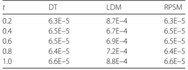
Comparison of absolute errors of the presented DT technique with LDM and RPSM for N= 2 is done in Tables1,2and3. We see that DT and RPSM produce the same results, which are close to the values of the closed form solutions, whereas LDM shows significant deviations. We obtain similar results when comparing computing times, see Tables4,5
and6.
Remark4 In [29], the authors used LDM and obtained only approximate solutions of the initial value problem (12), (13). Applying RPSM, the authors were able to find closed-form solutions in [30]. However, the calculations are too complicated, and the residual functions (RPSM) and initial guesses (LDM) contain analytical forms of functionssinandcos, which means that these methods are not convenient for use in a purely numerical software.
Table 4 Comparison of computing time foru1
t DT LDM RPSM
0.2 6.3E–5 8.7E–4 6.3E–5
0.4 6.5E–5 6.7E–4 6.5E–5
0.6 6.5E–5 6.9E–4 6.5E–5
0.8 6.4E–5 7.2E–4 6.4E–5
1.0 6.6E–5 8.8E–4 6.6E–5
Table 5 Comparison of computing time foru2
t DT LDM RPSM
0.2 6.6E–5 6.7E–4 6.6E–5
0.4 6.4E–5 6.7E–4 6.4E–5
0.6 6.7E–5 6.7E–4 6.7E–5
0.8 6.5E–5 8.5E–4 6.5E–5
1.0 6.5E–5 8.3E–4 6.5E–5
Table 6 Comparison of computing time foru3
t DT LDM RPSM
0.2 6.6E–5 7.7E–4 6.6E–5
0.4 6.7E–5 6.6E–4 6.7E–5
0.6 6.6E–5 6.7E–4 6.6E–5
0.8 6.6E–5 8.3E–4 6.6E–5
1.0 6.7E–5 8.5E–4 6.7E–5
Example2 Let us solve a nonlinear system of neutral delayed differential equations
u1 =u1(t– 2)u1
fort∈[–2, 0], and initial conditions
u1(0) = 1, u1(0) = 1, u1(0) = 1,
u2(0) = 0, u2(0) = 0, u2(0) = 2.
(17)
Following the method of steps, we get
u1 =e(t–2)u1
System (18) cannot be solved by the classical DT approach because of the nonlinear term f(u) =3
components to the nonlinear termf(u). Applying DT to (18), we get the system mula (4) and the transformed initial conditions
U1(0) = 1, U1(1) = 1, U1(2) =
Solving the system of recurrence relations (19)–(20), we get
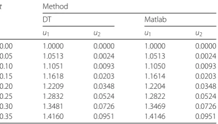
Table 7 Comparison of values of solution components obtained by DT and Matlab
t Method
DT Matlab
u1 u2 u1 u2
0.00 1.0000 0.0000 1.0000 0.0000
0.05 1.0513 0.0024 1.0513 0.0024
0.10 1.1051 0.0093 1.1050 0.0093
0.15 1.1618 0.0203 1.1614 0.0203
0.20 1.2209 0.0348 1.2204 0.0348
0.25 1.2832 0.0524 1.2822 0.0524
0.30 1.3481 0.0726 1.3469 0.0726
0.35 1.4160 0.0951 1.4146 0.0951
Table 8 Comparison of computing time
t Method
DT Matlab
u1 u2 u1 u2
0.05 7.9E–5 6.5E–5 6.2E–2 6.2E–2
0.10 6.9E–5 7.0E–5 8.1E–2 6.2E–2
0.15 7.1E–5 6.8E–5 6.2E–2 6.2E–2
0.20 7.0E–5 6.9E–5 6.3E–2 6.2E–2
0.25 7.0E–5 7.0E–5 6.2E–2 6.2E–2
0.30 6.3E–5 6.9E–5 6.3E–2 6.3E–2
0.35 6.9E–5 6.8E–5 6.2E–2 6.3E–2
Applying the inverse differential transformation, we obtain an approximate solution to the initial value problem (15)–(17):
u1(t) = 1 +t+
1 2t
2+2 +e–2
6 t
3+4e–2+5
72 t
4+16e–2–5
1080 t
5+· · ·,
u2(t) =t2–
2 3t
3+ 2
27t
4+ 2
189t
5+· · ·.
As we do not know the exact solution of the given problem, we are limited to compar-ing approximate solutions. Comparison of values obtained by the proposed approach and values obtained by Matlab package DDENSD in Table7shows good correspondence be-tween the results. Comparing computing times in Table8, we can see that the presented method produces reliable results much faster than Matlab package DDENSD.
Remark5 System (15) contains all three types of delay which were considered in this pa-per. Moreover, it contains a term which is nonlinear (nonpolynomial) in the dependent variableu1. In this sense, the present paper contains more complicated systems in
appli-cations than papers about other semi-analytical methods like VIM [6], ADM [7] or HPM [8].
5 Conclusions
with respect to the problem studied in [20]. The comparison of results was done against the Laplace decomposition method, residual power series method and Matlab package DDENSD. The need of computational work is reduced compared to the other methods. The differential transformation algorithm gives an approximate solution which is in good concordance with reference results produced by Matlab. Under certain circumstances, it is possible to identify the unique solution to the initial value problem in closed form. Fur-ther steps can be done in the development of the presented technique for systems with distributed and state dependent delays.
Funding
The first author was supported by the Grant CEITEC 2020 (LQ1601) with financial support from the Ministry of Education, Youth and Sports of the Czech Republic under the National Sustainability Programme II. The work of the second author was supported by the Grant FEKT-S-17-4225 of Faculty of Electrical Engineering and Communication, Brno University of Technology.
Competing interests
The authors declare that they have no competing interests.
Authors’ contributions
All authors contributed equally to the writing of this paper. All authors read and approved the final manuscript.
Author details
1CEITEC BUT, Brno University of Technology, Brno, Czech Republic.2Faculty of Electrical Engineering and
Communication, Brno University of Technology, Brno, Czech Republic.
Publisher’s Note
Springer Nature remains neutral with regard to jurisdictional claims in published maps and institutional affiliations.
Received: 12 October 2018 Accepted: 15 January 2019 References
1. Györi, I.: Oscillation and comparison results in neutral differential equations and their applications to the delay logistic equation. Comput. Math. Appl.18(10–11), 893–906 (1989)
2. Insperger, T., Milton, J., Stepan, G.: Semidiscretization for time delayed neural balance control. SIAM J. Appl. Dyn. Syst. 14(3), 1258–1277 (2015)
3. Kalmar-Nagy, T., Stepan, G., Moon, F.C.: Subcritical Hopf bifucration in the delay equation model for machine tool vibrations. Nonlinear Dyn.26, 121–142 (2011)
4. Hale, J.K., Verduyn Lunel, S.M.: Introduction to Functional Differential Equations. Springer, New York (1993)
5. Kolmanovskii, V., Myshkis, A.: Introduction to the Theory and Applications of Functional Differential Equations. Kluwer Academic, Dordrecht (1999)
6. Chen, X., Wang, L.: The variational iteration method for solving a neutral functional-differential equation with proportional delays. Comput. Math. Appl.59, 2696–2702 (2010)
7. Blanco-Cocom, L., Estrella, A.G., Avila-Vales, E.: Solving delay differential systems with history functions by the Adomian decomposition method. Appl. Math. Comput.218, 5994–6011 (2013)
8. Shakeri, F., Dehghan, M.: Solution of delay differential equations via a homotopy perturbation method. Math. Comput. Model.48, 486–498 (2008)
9. Duarte, J., Januario, C., Martins, N.: Analytical solutions of an economic model by the homotopy analysis method. Appl. Math. Sci.10(49), 2483–2490 (2016)
10. Rebenda, J., Šmarda, Z.: A semi-analytical approach for solving nonlinear systems of functional differential equations with delay. In: Simos, T.E. (ed.) 14th International Conference of Numerical Analysis and Applied Mathematics (ICNAAM 2016). AIP Conference Proceedings, vol. 1863, p. 530003. AIP Publishing, Melville (2017)
11. Bellour, A., Bousselsal, M.: Numerical solution of delay integro-differential equations by using Taylor collocation method. Math. Methods Appl. Sci.37, 1491–1506 (2014)
12. Sezer, M., Akyuz-Dascioglu, A.: Taylor polynomial solutions of general linear differential-difference equations with variable coefficients. Appl. Math. Comput.174, 753–765 (2006)
13. Cherepennikov, V.B., Ermolaeva, P.G.: Smooth solutions of an initial-value problem for some differential difference equations. Numer. Anal. Appl.3, 174–185 (2010)
14. Cherepennikov, V.B.: Numerical analytical method of studying some linear functional differential equations. Numer. Anal. Appl.6, 236–246 (2013)
15. Jain, R.K., Agarwal, R.P.: Finite difference method for second order functional differential equations. J. Math. Phys. Sci. 7(3), 301–3016 (1973)
16. Agarwal, R.P., Chow, Y.M.: Finite-difference methods for boundary-value problems of differential equations with deviating arguments. Comput. Math. Appl.12A(11), 1143–1153 (1986)
18. Petropoulou, E.N., Siafarikas, P.D., Tzirtzilakis, E.E.: A “discretization” technique for the solution of ODEs II. Numer. Funct. Anal. Optim.30, 613–631 (2009)
19. Šamajová, H., Li, T.: Oscillators near Hopf bifurcation. Komunikácie (Žilina)17, 83–87 (2015)
20. Rebenda, J., Šmarda, Z.: A differential transformation approach for solving functional differential equations with multiple delays. Commun. Nonlinear Sci. Numer. Simul.48, 246–257 (2017)
21. Yang, X.-J., Tenreiro Machado, J.A., Srivastava, H.M.: A new numerical technique for solving the local fractional diffusion equation: two-dimensional extended differential transform approach. Appl. Math. Comput.274, 143–151 (2016)
22. Šamajová, H.: Semi-analytical approach to initial problems for systems of nonlinear partial differential equations with constant delay. In: Mikula, K., Sevcovic, D., Urban, J. (eds.) Proceedings of EQUADIFF 2017 Conference, pp. 163–172. Spektrum STU Publishing, Bratislava (2017)
23. Rebenda, J., Šmarda, Z., Khan, Y.: A new semi-analytical approach for numerical solving of Cauchy problem for differential equations with delay. Filomat31(15), 4725–4733 (2017)
24. Šmarda, Z., Diblík, J., Khan, Y.: Extension of the differential transformation method to nonlinear differential and integro-differential equations with proportional delays. Adv. Differ. Equ.2013, 69 (2013)
25. Šmarda, Z., Khan, Y.: An efficient computational approach to solving singular initial value problems for Lane–Emden type equations. J. Comput. Appl. Math.290, 65–73 (2015)
26. Rebenda, J.: An application of Bell polynomials in numerical solving of nonlinear differential equations. In: 17th Conference on Applied Mathematics, APLIMAT 2018—Proceedings, pp. 891–900. Spektrum STU, Bratislava (2018) 27. Bellen, A., Zennaro, M.: Numerical Methods for Delay Differential Equations. Oxford University Press, Oxford (2003) 28. Warne, P.G., Polignone Warne, D.A., Sochacki, J.S., Parker, G.E., Carothers, D.C.: Explicit a-priori error bounds and
adaptive error control for approximation of nonlinear initial value differential systems. Comput. Math. Appl.52, 1695–1710 (2006)
29. Widatalla, S., Koroma, M.A.: Approximation algorithm for a system of pantograph equations. J. Appl. Math.9, Article ID 714681 (2012)
![Table 2 Error analysis of u2 on [0,1]](https://thumb-us.123doks.com/thumbv2/123dok_us/937706.1114092/8.595.118.480.223.301/table-error-analysis-of-u-on.webp)