R E S E A R C H
Open Access
Analysis on LUT based digital
predistortion using direct learning architecture
for linearizing power amplifiers
Xiaowen Feng
1,2, Yide Wang
1,3, Bruno Feuvrie
1,4, Anne-Sophie Descamps
1,4, Yuehua Ding
5,3*and Zhiwen Yu
3,6Abstract
In modern wireless communication system, power amplifier (PA) is an important component which is expected to be operated at the region of high power efficiency, but in this region, PA is inherently nonlinear. Thus, the linearization of high power efficient PA is necessary. In this paper, direct learning architecture (DLA) and indirect learning architecture (ILA) are firstly compared. It shows that DLA is more robust than ILA. Then a baseband digital predistortion (DPD) method with DLA is proposed for power amplifier linearization based on combined look-up tables (LUT) and memory polynomial (MP) model. The main innovation is that a LUT-based approach is proposed to calculate directly the complex-valued predistorted signal. Moreover, some interpolation techniques are introduced to reduce the LUT size. The proposed DPDs are validated experimentally. Additionally, the influences of some important parameters in experimental setup, such as the number of bits of analog-to-digital converter (ADC) and the instrument bandwidth, are analyzed.
Keywords: Baseband digital predistortion, Power amplifiers, Memory polynomial, Look-up table
1 Introduction
In modern wireless communication system, the energy consumption is an extremely important issue, especially for the transmitter. Power amplifier (PA) is a crucial com-ponent in the transmitter. Generally, for achieving a good power efficiency, PA must operate close to its compres-sion region. Unfortunately, the high spectral efficiency signals used by today’s wireless communication systems are characterized by their non-constant envelopes and high peak-to-average power ratio (PAPR). Their ampli-tudes may overtop the compression region of the PA. The resulting nonlinear distortions, such as the spec-tral regrowth and degradation of error vector magnitude (EVM), disturb the transmission. Moreover, to support
*Correspondence: [email protected]
5School of Electronic and Information Engineering, South China University of Technology, Wushan Road, Tianhe District, Guangzhou, Peoples Republic of China
3Sino-French Research Center in Information and Communication (SFC/RIC), Rue Christian Pauc, Nantes, France
Full list of author information is available at the end of the article
more users and provide higher data rates, the bandwidth of signal continues to increase. PA exhibits stronger mem-ory effects with the increasing of the bandwidth of signal [1]. The research on high power efficient PA driven by a wide bandwidth signal is of great practical significance [2, 3]. To compensate PA nonlinearities, several lineariza-tion techniques are developed, such as feed-forward, feedback, linear amplification with nonlinear compo-nents (LINC) and predistortion techniques. Among these techniques, predistortion technique, particularly base-band digital predistortion (DPD), has been widely studied thanks to its ability of reconfiguration and simplicity of implementation.
DPD is one of the most effective linearization tech-niques. Its principle is to insert a digital predistorter (PD) in front of PA, which has the inverse nonlinear char-acteristics of that of the PA, so that the cascaded PD-PA system has a linear behavior. DPD can be realized using two architectures [4–6]: indirect learning archi-tecture (ILA) and direct learning archiarchi-tecture (DLA). In ILA approach [7], a postdistorter model is first assumed, the measured output of PA is taken as the input of the
postdistorter, and the measured input of PA is taken as the output of the postdistorter. Then, the postdistorter is estimated by an identification algorithm such as least squares (LS) method. Finally, the identified postdistorter is placed directly in front of PA as the predistorter. In DLA approach [8–10], a model of PA’s behavior is first defined, then its coefficients are identified, and finally the predistorter is found by reversing the identified PA model.
Among various DPD techniques, three solutions are popularly used. They are look-up table (LUT), polyno-mial model and neural network based DPDs. In [11, 12], several neural network-based DPDs have been proposed. The neural network has an excellent capability to accu-rately approximate nonlinear functions. Hence, it can be used to linearize the PA. But the training process of neural network is complex and time-consuming. Its hard-ware implementation is difficult in practical applications. LUT [13–16] based DPD has the advantage of simplic-ity, but its linearization performance depends on the LUT size. In order to improve the linearization performance with limited LUT dimension, some interpolated tech-niques are introduced in LUT-based DPDs. Polynomial [7, 8, 17] model-based DPD is also widely studied in the literature. They include the well-known Volterra series (VS) [18], memory polynomial (MP) [7, 8, 13], gener-alized memory polynomial (GMP) [19], other simplified VS variants [20] and so on. VS and GMP models are more accurate but also more complex. MP model has lower complexity and can closely mimic the nonlinear behavior of the PA with memory effects. It offers a good tradeoff between computational complexity and modeling accuracy.
In [7], a MP based DPD with indirect learning archi-tecture is presented, where the MP model performs robustly and the model’s parameters are easy to extract. But compared with the DPD with direct learning archi-tecture, the DPD with indirect learning architecture is less robust in the presence of noise [4]. In [10], a MP-based DPD with direct learning architecture is proposed, where it uses a root-finding method to calculate the predistorted signal. This DPD can achieve excellent lin-earization performance but the root-finding procedure is time-consuming. In [13], a MP/LUT DPD is proposed, where a conventional LUT is used instead of the root-finding procedure. The calculating time of DPD process decreases greatly but it requires a sufficiently large size of LUT.
In our previous work [21, 22], some interpolated LUTs are introduced based on MP/LUT DPD. Thanks to the interpolation techniques, the improved DPDs achieve good performance in terms of computational efficiency and LUT size. In [21], the linear interpola-tion is introduced based on MP/LUT DPD. In [22], the
quadratic-interpolated LUT is combined with the non-uniform MP model. It is worth noting that, in [21, 22], LUTs are only used to determine the amplitude of the predistorted signal. While the predistorted signal’s phase must be calculated by another separated time-consuming process. In [23], the two interpolated LUTs are used based on non-uniform MP model. The linear-interpolated LUT is used to determine the amplitude of the pre-distorted signal. And, the quadratic-interpolated LUT is used to determine the phase of the predistorted signal. In this paper, we propose three LUT-based methods: LUT-based, LILUT-based, and QILUT-based methods. In the LUT-based method, the amplitude and phase of the predistorted signal both are calculated by a single clas-sical LUT. In the LILUT-based method, the amplitude and phase of the predistorted signal both are calculated by a single linear-interpolated LUT. In the QILUT-based method, the amplitude and phase of the predistorted signal both are calculated by a single quadratic-interpolated LUT.
Additionally, in practical implementation, the lineariza-tion performance of DPDs is directly related to the num-ber of bits of ADC (analog-to-digital converter) and the bandwidth of instruments [24]. This important issue is also studied in this paper.
The remainder of this paper is organized as follows. Section 2 presents the principles of ILA and DLA, and makes a comparison between them. The proposed DPD solution is presented in Section 3. Section 4 discusses some practical problems in the measurements, especially the influence of signal bandwidth. The experimental setup and results are presented in Section 5. Finally, Section 6 concludes the paper.
2 Predistortion architectures
In this section, the details of ILA and DLA are pre-sented. And, the two architectures are compared by some simulations.
2.1 Indirect learning architecture
Figure 1 shows the block diagram of ILA. Firstly, the postdistorter is identified. Usually, the postdistorter is modeled as a MP [4]. The output of the postdistorter can be expressed as
Fig. 1Indirect learning architecture
signalsx(n)andy(n)are the measured input and output of PA, respectively. Assume that the total number of samples isN, we get
zp=Za (2)
where zp =[zp(1),· · ·,zp(N)]T,Z =[u00,· · ·,u0L,· · ·,
ukl,· · ·,uK0,· · ·,uKL]N×(K+1)(L+1),ukl=[kl[z(1)] ,· · ·, kl[z(N)] ]T, anda=[a00,· · ·,a0L,· · ·,akl,· · ·,aK0,· · ·,
aKL]T. Classical LS method can be used to extract the
coefficients
ˆ
a=ZHZ−1ZHzp (3)
where(·)Hdenotes the complex conjugate transpose oper-ation. After the identification of the postdistorter, the copy of the postdistorter is placed directly in front of PA as the predistorter.
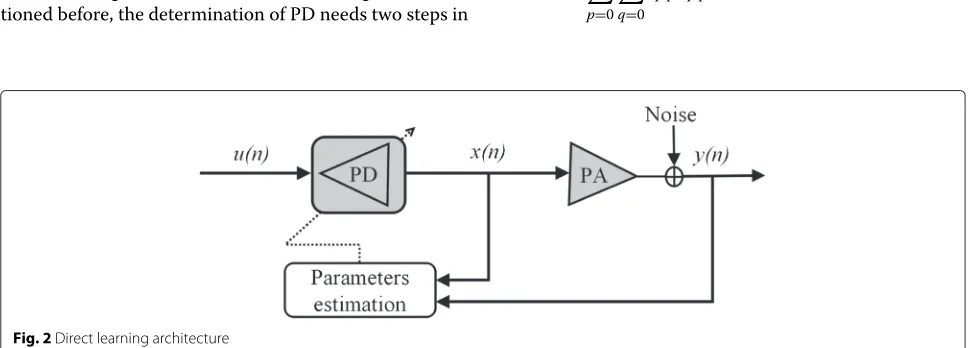
2.2 Direct learning architecture
The block diagram of DLA is illustrated in Fig. 2. As men-tioned before, the determination of PD needs two steps in
DLA. Firstly, the model of PA’s behavior needs to be pre-defined. Here, MP is adopted as the PA model. The PA model is defined as
y(n)=
P
p=0
Q
q=0
cpqpq[x(n)] (4)
wherepq[x(n)]=x(n−p)x(n−p)2q,Pand 2Q+1 are
the memory depth and highest nonlinearity order, respec-tively, andcpqare the model’s coefficients. The signalsx(n)
andy(n)are the input and output of PA, respectively. The coefficientscpqare extracted by LS method as mentioned
before. Secondly, the identified model of PA is reversed for the determination of PD. In the following, the method in [10] to determine the PD with DLA is described.
The ideal cascaded PD-PA system can be expressed as
y(n)=
P
p=0
Q
q=0
cpqpq[x(n)]=G0u(n) (5)
where u(n) denotes the input of the PD-PA system and x(n)the predistorted signal (also the input of PA). Accord-ing to the memory behavior of PA, the outputy(n)of PA can be represented as the sum of two parts: the static part s(n)depending only on the current input sample (p= 0), and the dynamic partd(n)which depends on the previous input samples (pfrom 1 toP). the predistorted signal x(n), respectively. By definition, d(n) depends only on the previous samples, the right-hand side of (7) and coefficientsc0qare known at instant
n. The amplitude|x(n)|of the predistorted signal can be calculated by taking the absolute value.
Equation (8) is a high-order nonlinear equation, the amplitude|x(n)|of the predistorted signal can be found by a root-finding procedure [10]. The corresponding phase ∠x(n)is then calculated by
Finally, the predistorted signalx(n)is given by
x(n)= |x(n)|ej∠x(n). (10)
2.3 Comparison of ILA and DLA
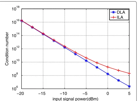
Two different DPD architectures (ILA and DLA) are pre-sented in the above subsection. They both need to identify a pre-assumed model (MP model) with the measured input and output of PA. LS method is used in the model identification. From (3), it can be seen that the inverse of ZHZ is required in LS algorithm. When solving the inverse problem, the condition number is usually used to measure how sensitive the solution is to changes or errors in the input. A problem with a low condition number is said to be well-conditioned, while a problem with a high condition number is said to be ill-conditioned.
In this subsection, the condition number of ZHZ is considered to measure the stability of the two DPD architectures. In ILA, Zis related to the output signal of PA. While in DLA, it is related to the input sig-nal of PA. A simulation is realized to compare these
−20 −15 −10 −5 0 5
Fig. 3Comparison of condition number with different input signal power
two DPD architectures. In this simulation, a Wiener model is used as PA model. It is implemented as a three-tap FIR filter with coefficients [0.7692, 0.1538, 0.0769] [25], followed by a Saleh model. Saleh model is described as
[26]. The input signal of PA is a WCDMA signal with 3.84 MHz bandwidth. The measured sequence has 1000 symbols (8000 samples). The ideal gain of this PA model is about 26 dB. The input power at 1 dB compression point is about−1 dBm.
The condition number of ZHZis affected byZwhich depends on the memory depth, nonlinearity order and value of each element (varies with the input signal power). In the first simulation, we assume that the memory depth is 3 (K = P = 3) and the nonlinearity order is 5 (L = Q = 2). The signal input power varies from−20 to 5 dBm. The condition numbers ofZHZof two DPD architectures are compared. The results are shown in Fig. 3.
In the second simulation, we assume that the input sig-nal power is 0 dBm. The nonlinearity order varies from 3 to 15. The memory depth varies from 0 to 3. The comparison of two DPD architectures is shown in Fig. 4.
2 4 6 8 10 12 14 16 100
105 1010 1015 1020 1025
Nonlinearity order
Condition number
DLA,memory depth=0 ILA,memory depth=0 DLA,memory depth=1 ILA,memory depth=1 DLA,memory depth=2 ILA,memory depth=2 DLA,memory depth=3 ILA,memory depth=3
Fig. 4Comparison of condition number with different nonlinearity orders and memory depthes
In practical measurement, an ADC is required to realize the signal acquisition. The number of bits of ADC will affect the accuracy of the signal acquisition and then affect the performance of the model’s iden-tification. Additionally, the measurement at the output of PA is noisy in practical application. The noise also affects the performance of the model’s identification. In the third simulation, these two DPD architectures are compared in terms of the number of bits of ADC in signal acquisition and the noise power at the output of PA.
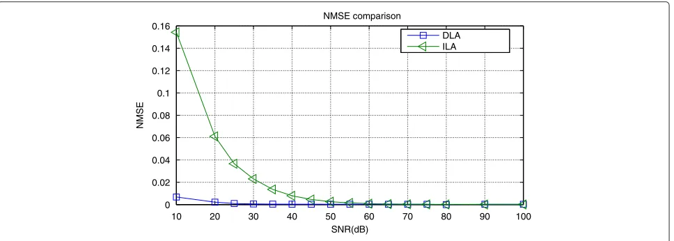
For analyzing the influence of the noise at the output of PA, it assumes that complex white Gaussian noise is
present at the output of PA as shown in Figs. 1 and 2. An original WCDMA signalx(n)(bandwidth 3.84 MHz, power 0 dBm, sequence length 8000 samples) is given as the PA input. And the outputy(n) of PA is obtained by the Wiener model. The white Gaussian noise is added in the output signaly(n) to get the noisy outputynoise(n). The inputx(n) and output ynoise(n) of PA are used for the model identification of (1) and (4). In this process, we takeK = P = 3 (memory depth=3) andL = Q = 2 (nonlinearity order=5), respectively.
After the model identification, another WCDMA sig-nal x(n) is used to test the identified model. For the inputx(n), the corresponding outputy(n)is obtained.
10 20 30 40 50 60 70 80 90 100
0 0.02 0.04 0.06 0.08 0.1 0.12 0.14 0.16
SNR(dB)
NMSE
NMSE comparison
DLA ILA
2 4 6 8 10 12 14 16 0
0.005 0.01 0.015 0.02
Number of bits of ADC
NMSE
NMSE comparison
DLA ILA
Fig. 6Comparison of ILA and DLA when considering the number of bits of ADC
For ILA, the signaly(n)is the input of the postdistorter, its output zp(n) is obtained by the identified model (1). The normalized mean squared error (NMSE) between zp(n)andx(n)is treated as the criterion of ILA model-ing accuracy. For DLA, the signalx(n)is the input of the identified model (4), the corresponding outputyDLA(n)is obtained. The normalized mean squared error (NMSE) betweenyDLA(n)andy(n)is treated as the criterion of DLA modeling accuracy. Figure 5 shows the performance of ILA and DLA in terms of NMSE when the noise is present. It can be seen that the modeling accuracy of ILA and DLA both improves as the noise power decreases. When the noise is high, the performance of DLA is better than that of ILA. When the power of noise is low (nearly ideal case), the performance of DLA and ILA is similar. In practical applications, the noise can not be ignored. DLA is more robust than ILA when the noise is present.
For the influence of the number of bits of ADC, an ADC is assumed for the signal acquisition. The signals x(n)
andy(n)pass the ADC and are denoted byxADC(n)and yADC(n), respectively. The signalsxADC(n) andyADC(n) are used for the model identification of (1) and (4). The same signalx(n)is used to test the identified model. The comparison principle considering the number of bits of ADC is the same as that considering the noise. Figure 6 shows the performance of ILA and DLA in terms of NMSE with varying number of bits of ADC. It can be seen that the modeling accuracy of ILA and DLA both improves as the number of bits of ADC increases. The modeling accuracy of DLA is always better than that of ILA.
According to the above analysis, it further verifies that DLA is more robust than ILA with respect to perturba-tions. Finally, the two DPDs based on different learning architectures are compared for the validation. The DPD proposed in [7] is taken as the example of ILA. And, the DPD proposed in [10] is taken as the example of DLA. In this simulation, the number of bits of ADC and the noise
−500 −40 −30 −20 −10 0 10
200 400 600 800 1000 1200 1400
Input power (dBm)
Number
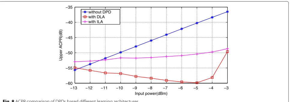
−13 −12 −11 −10 −9 −8 −7 −6 −5 −4 −3 −60
−55 −50 −45 −40 −35
Input power(dBm)
Upper ACPR(dB)
without DPD with DLA with ILA
Fig. 8ACPR comparison of DPDs based different learning architectures
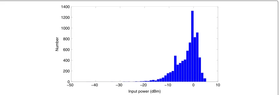
both are taken into account in the process of identifica-tion. We assume that the number of bits of ADC is 8, the SNR at the output of PA is 35 dB. The average power of the input signal varies from−13 to−3 dBm. The input signal, which has an average power of−3 dBm, includes many samples entering the nonlinear region of PA model. Figure 7 illustrates the distribution of samples of the input signal when its average power is−3 dBm. It shows that the power of about 40 % of the input samples is higher than the input power (−1 dBm) at 1 dB compression point of the PA model.
The original input x(n) and output y(n) of PA pass firstly the ADC, then the noise is added on the out-put signal of PA. The processed inout-put and outout-put signals are used for the model identification of (1) and (4). For ILA, the identified postdistorter model is directly placed in front of PA as the predistorter [7]. For DLA, the predistorter is determined by inverting the identified PA model [10].
The linearized outputs of the two different learning architectures are obtained by the DPD solutions stated above. The adjacent channel power ratio (ACPR) and EVM of linearized outputs of two architectures are calcu-lated, respectively. Figure 8 shows the evolution of ACPR of linearized outputs with varying input power. And, Fig. 9 shows the evolution of EVM of linearized outputs with varying input power. It can be seen that the linearization performance of DLA is much better than that of ILA when considering the number of bits of ADC and the noise at the output of PA. Consequently, in this paper, DPD based on DLA is adopted.
3 Proposed LUT-based digital predistortion
In this section, the details of the proposed DPD are presented. In Section 2.2, a MP-based DPD with DLA is described. The calculation of the predistorted signal includes two parts: the amplitude and phase. The ampli-tude and phase of the predistorted signal are calculated by
−13 −12 −11 −10 −9 −8 −7 −6 −5 −4 −3
0 2 4 6 8 10
Input power(dBm)
EVM(%)
without DPD with DLA with ILA
Table 1Values of LUT
LUT input LUT output
E(0) R(0)ejθ(0)
. . . . . .
E(m) R(m)ejθ(m)
. . . . . .
E(M) R(M)ejθ(M)
(8) and (9), respectively. In [13, 21, 22], only the amplitude calculation in (8) is considered. The approaches based on LUT are used instead of the root-finding process. Actu-ally, the process of calculating the phase in (9) is also time-consuming. In this paper, an approach based on LUT is proposed to calculate the amplitude and also the phase of the predistorted signal. The proposed approach is presented as follows. (9) can be rewritten as
∠x(n)=arg{G0u(n)−d(n)}
Before performing the predistortion, a LUT including the information of the amplitude and phase of the predis-torted signal should be constructed. Firstly, the dynamic range of the amplitude |x(n)| of the predistorted sig-nal is estimated according to the maximum amplitude of the original input signal u(n) and the saturation input amplitude of PA. Then the maximum range of|x(n)|is decomposed intoM+1 intervals with equal length (the length of each interval is equal tox), denoted byR(m). The LUT is shown in Table 1. In this table,
R(m)=mx (13)
After the LUT is constructed, the predistortion algo-rithm is described in Algoalgo-rithm 1.
Algorithm 1Proposed DPD based on simple LUT
1. Initializen=0,d(0)=0.
The proposed approach based on a simple LUT can significantly improve the time efficiency of DPD pro-cess than the corresponding root-finding approach, but its linearization performance is proportional to the table size. To obtain good linearization performance, the table size must be sufficiently large. Therefore, some interpola-tion techniques should be introduced in the simple LUT. The linear interpolation and the quadratic interpolation
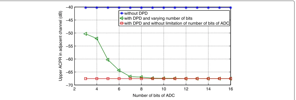
2 4 6 8 10 12 14 16
Number of bits of ADC
Upper ACPR in adjacent channel (dB)
without DPD
with DPD and varying number of bits
with DPD and without limitation of number of bits of ADC
0 2 4 6 8 10 12 14 16 18 20 −80
−75 −70 −65 −60 −55 −50 −45 −40
Cutoff frequency/Singal bandwidth
Upper ACPR in adjacent channel (dB)
without DPD
with DPD and bandwidth limitation with DPD and without bandwidth limitation
Fig. 11Evolution of adjacent channel ACPR versus cutoff frequency
are adopted in LUT, respectively. The linear-interpolated LUT and quadratic-interpolated LUT will be denoted in the rest of the paper as LILUT and QILUT, respectively. The algorithm of proposed DPD based on LILUT is differ-ent from that based on simple LUT at the step 4). For the algorithm of proposed DPD based on LILUT, the step 4) is as follows
x(n)=LILUT{E(m)} =R(m)ej{arg{s(n)}−θ(m)} (16) whereLILUT is the linear-interpolated LUT [21]. Simi-larly, for the algorithm of proposed DPD based on QILUT,
the step 4)is as follows
x(n)=QILUT{E(m)} =R(m)ej{arg{s(n)}−θ(m)} (17) whereQILUTis the quadratic-interpolated LUT [22].
In this section, three DPD approaches are described. For convenience, the proposed DPDs based on sim-ple LUT, LILUT and QILUT are called as LUT-based, LILUT-based, and QILUT-based, respectively. Among these three approaches, it is difficult to judge which one is the best, since they provide different degrees of trade-off between the linearization performance, table size and time efficiency.
Fig. 13Photograph of experimental setup
4 Discussions
In order to validate the proposed DPDs, experimental measurements are necessary. Before the measurements, some problems are discussed. In practical measurements, hardware conditions can not be ignored, such as the num-ber of bits of ADC and instrument bandwidth. In the following, these parameters are analyzed by some sim-ulations. In the simulations, the original input signal is a WCDMA signal with 3.84 MHz bandwidth. The input sequence is 1000 symbols. The input power is−5 dBm. The PA model is the Wiener PA model mentioned in Section 2.3. The DPD method used is the root-finding-based DPD [10].
For the problem of number of bits of ADC, as mentioned before, an ADC is assumed before the data
acquisition. The number of bits of ADC varies form 3 to 16. And the sampling frequency of the input signal is eight samples/symbol. The ACPR is used to quantify the linearization performance. Figure 10 presents the evolu-tion of ACPR versus the number of bits of ADC. It can be seen that the linearization performance improves as the number of bits of ADC increases. It indicates that if the number of bits of ADC is not big enough in the data acquisition, the quantization error is too large and degrades the linearization performance. Additionally, the number of bits of ADC should not be too high. In this paper, the acquisition of signals by Agilent E4440A is realized with ADC of 14 bits in the experimental setup. The experimental setup will be presented in the next section.
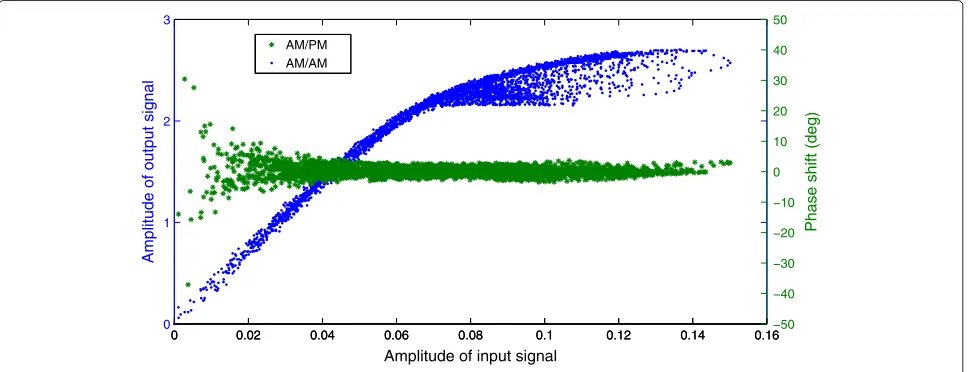
0 0.02 0.04 0.06 0.08 0.1 0.12 0.14 0.16
0 1 2 3
Amplitude of output signal
Amplitude of input signal
0 0.02 0.04 0.06 0.08 0.1 0.12 0.14 0.16−50
−40 −30 −20 −10 0 10 20 30 40 50
Phase shift (deg)
AM/PM AM/AM
Another problem is the bandwidth of instrument. In simulations, the signal bandwidth is only limited by the sampling frequency. In the measurement, except for the influence of the sampling frequency, the signal band-width is also affected by the bandband-width of instrument. When the bandwidth of instrument is narrower than that of the signal, the signal passing the instrument will be distorted. Especially, the signal bandwidth will increase after the predistortion. The bandwidth of the predistorted signal is wider than that of the original input signal. Thus, if the bandwidth of instrument is not sufficiently wide, the desired predistortion will be not achieved.
In order to evaluate the required bandwidth, the fol-lowing simulation is made. It assumes that the sampling frequency of input signal is 50 samples/symbol. To sim-ulate the instrument limitation, a lowpass linear-phase filter, with order 200 and a varying cutoff frequency, is used to limit the bandwidth of the predistorted signal. The limited bandwidth signal is finally applied to the Wiener PA model.
Figure 11 presents the evolution of ACPR versus the cutoff frequency, where this cutoff frequency rep-resents the bandwidth of instrument. It indicates that only the bandwidth of instrument is wide enough (at least 5 times), the linearization performance will be perfect.
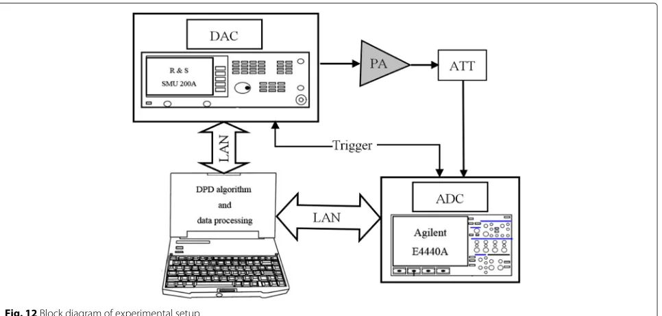
5 Experimental results
In order to validate the proposed DPDs, an experimental testbed is built. Figures 12 and 13 show the used exper-imental testbed. It consists of a PA (ZFL 2500), a PC providing the baseband signal and realizing DPD algo-rithms, a vector signal generator (Rohde & Schwarz SMU 200 A) to generate the RF signal and a spectrum ana-lyzer (Agilent E4440A, 3 Hz − 26.5 GHz) to analyze the input and output signals of PA. For PA ZFL2500, it has 500–2500 MHz bandwidth and about 31 dB gain. The average output power at 1 dB compression point is around 17 dBm at frequency of 1.8 GHz. Figure 14 shows AM/AM and AM/PM characteristics of PA ZFL2500.
The proposed approach, LUT-based, LILUT-based, and QILUT-based DPDs, all are tested on this experimen-tal testbed. The root-finding-based DPD in [10] is com-pared with the proposed three DPD approaches. The performance is evaluated in terms of the linearization capability, time efficiency and table size. The lineariza-tion capability is measured by two parameters. One is the NMSE between the predistorted signals by the three LUT based DPDs and the predistorted signal by root-finding-based DPD. The other is the measured ACPR at the output of linearized PA. The time effi-ciency refers to the consumed time of DPD process
Table 2NMSE of predistorted signals and time comparisons using different DPD methods
DPDs NMSE (dB) Time (us)
Root-finding-based DPD −∞ 103.75
LUT-based DPD (size 30) –34.18 9.63
LUT-based DPD (size 1000) –65.39 11.38
LILUT-based DPD (size 10) –61.20 20.75
LILUT-based DPD (size 30) –81.59 21.38
QILUT-based DPD (size 10) –75.93 71.25
QILUT-based DPD (size 20) –94.89 72.88
for obtaining one predistorted sample x(n) as shown in Algorithm 1. The table size refers to the chosen size of LUT.
For these measurements, PA ZFL2500 is driven by a WCDMA signal with 3.8 MHz bandwidth. The sampling frequency is 20 samples/symbol. The signal sequence has 200 symbols (4000 samples). The considered MP model has a memory depth and nonlinearity order of 3 and 5, respectively. The NMSE between the predistorted signal by the proposed LUT-based DPD and the predistorted signal by root-finding-based DPD and consumed time of the proposed LUT-based DPD are summarized in Table 2. The power of original signal is−14 dBm (the correspond-ing output power is 17 dBm at the output of PA). It can be seen that the NMSE between the root-finding-based DPD and QILUT-root-finding-based DPD achieves−94.89 dB with table size of only 20. But, the consumed time of QILUT-based DPD is 72.88 us. It is higher than that of LILUT-based DPD (size 30) and that of LUT-based DPD (size 1000). The NMSE between the root-finding-based DPD and LILUT-based DPD achieves −81.59 dB when the table size is 30. The NMSE between the root-finding-based DPD and LUT-root-finding-based DPD only achieves−65.39 dB even if the table size is up to 1000. But it takes only 11.38
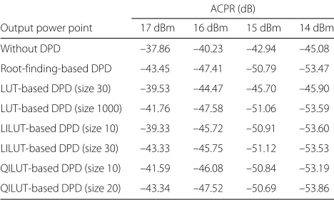
Table 3ACPR comparison using different DPD methods
ACPR (dB)
Output power point 17 dBm 16 dBm 15 dBm 14 dBm
Without DPD –37.86 –40.23 –42.94 –45.08
Root-finding-based DPD –43.45 –47.41 –50.79 –53.47
LUT-based DPD (size 30) –39.53 –44.47 –45.70 –45.90
LUT-based DPD (size 1000) –41.76 –47.58 –51.06 –53.59
LILUT-based DPD (size 10) –39.33 –45.72 –50.91 –53.60
LILUT-based DPD (size 30) –43.33 –45.75 –51.12 –53.53
QILUT-based DPD (size 10) –41.59 –46.08 –50.84 –53.19
−1 −0.5 0 0.5 1 x 10⁷ −70
−60 −50 −40 −30 −20 −10 0
Frequency (Hz)
PSD (dB)
w/o DPD
Root−finding−based DPD LUT−based DPD (size 30) LUT−based DPD (size 1000) LILUT−based DPD (size 30) QILUT−based DPD (size 20)
(a) Average output power 16 dBm
−1 −0.5 0 0.5 1
x 107 −70
−60 −50 −40 −30 −20 −10 0
Frequency (Hz)
PSD (dB)
w/o DPD
Root−finding−based DPD LUT−based DPD (size 30) LUT−based DPD (size 1000) LILUT−based DPD (size 30) QILUT−based DPD (size 20)
(b) Average output power 14 dBm
Fig. 15Comparison of several DPDs
us. The advantage of LUT-based DPD is its high time efficiency.
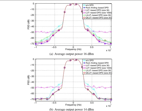
To compare ACPR values at the output of linearized PA, four average output power points are chosen : 17, 16, 15 and 14 dBm. The upper ACPR values of the output signals of different DPDs are measured and summarized in Table 3 (the offset of adjacent channel is set to be 5 MHz). Figure 15 shows the spectrums of output signals using different DPDs at the output power point 16 and 14 dBm. The ACPR values and spectrums further validate the results of Table 2. For LUT-based DPD, the lineariza-tion performance is very low when the table size is small. It achieves a similar linearization performance as the root-finding-based DPD with table size at least 1000. While LILUT-based DPD and QILUT-based DPD achieve the same performance as the root-finding-based DPD, with table size of only 30 and 20, respectively. In order to com-pare LILUT-based DPD and QILUT-based DPD clearly,
Fig. 16 shows their spectrums with the same table size 10 at the output power point 16 and 14 dBm. At the output power 16 dBm, the linearization performance of QILUT-based DPD is better than that of LILUT-based DPD. It is worth noting that, the linearization perfor-mance of QILUT-based DPD is a little worse than that of LILUT-based DPD at the output power 14 dBm. It is because the characteristic at the output power 14 dBm is more linear than that at the output power 16 dBm. LILUT-based DPD is better for the case where the prob-ability density of small signal is high (low nonlinearity). When the probability density of large signal is high, the nonlinearity increases, QILUT-based DPD can be selected.
6 Conclusions
−1 −0.5 0 0.5 1 x 10⁷ −70
−60 −50 −40 −30 −20 −10 0
Frequency (Hz)
PSD (dB)
w/o DPD
Root−finding−based DPD LILUT−based DPD (size 10) QILUT−based DPD (size 10)
(a) Average output power 16 dBm
−1 −0.5 0 0.5 1
x 107 −70
−60 −50 −40 −30 −20 −10 0
Frequency (Hz)
PSD (dB)
w/o DPD
Root−finding−based DPD LILUT−based DPD (size 10) QILUT−based DPD (size 10)
(b) Average output power 14 dBm
Fig. 16Comparison of LILUT-based DPD and QILUT-based DPD
of the condition number and considering the influence of the number of bits of ADC and noise in the signal mea-surement, it shows that DLA is more robust than ILA with respect to perturbations. The LUT-based, LILUT-based, and QILUT-based DPDs are then proposed for PA linearization based on MP model with DLA. These three DPDs allow some tradeoff between the linearization performance, time efficiency and table size. In different applications, a more appropriate DPD can be chosen to fit the actual situation. Moreover, the hardware condition of experimental setup is discussed. If a more accurate results are expected, a higher bits of ADC and a wider bandwidth of instrument are required.
Competing interests
This work is original research that has not been published previously, and not under consideration for publication elsewhere,in whole or in part.
Acknowledgements
This work was supported by the China Scholarship Council, the grant from Science and Technology Planning Project of Guangdong Province, China (No.
2015A050502011), the grant from National Natural Science Foundation of China (No. 61401157) and the grant from the funds of central universities (No. 2015ZM127).
Author details
1CNRS UMR6164, IETR, Ecole Polytechnique de l’universite de Nantes, Rue Christian Pauc, Nantes, France.2The 54th Research Institute of China Electronics Technology Group Corporation, Shijiazhuang, Peoples Republic of China.3Sino-French Research Center in Information and Communication (SFC/RIC), Rue Christian Pauc, Nantes, France.4IUT, GEII Nantes, Site Fleuriaye, Av. du Prof J. Rouxel, Carquefou, France.5School of Electronic and Information Engineering, South China University of Technology, Wushan Road, Tianhe District, Guangzhou, Peoples Republic of China.6School of Computer Science and Engineering, South China University of Technology, Wushan Road, Tianhe District, Guangzhou, Peoples Republic of China.
Received: 9 December 2015 Accepted: 29 April 2016
References
1. FM Ghannouchi, O Hammi, Behavioral modeling and predistortion. IEEE Microw. Mag.10(7), 52–64 (2009)
terminal applications. IEEE Trans. Microw. Theory Tech.60(5), 1321–1330 (2012)
3. O Hammi, A Kwan, S Bensmida, KA Morris, FM Ghannouchi, A digital predistortion system with extended correction bandwidth with application to LTE-A nonlinear power amplifiers. IEEE Trans. Circuits Syst. I Regular Papers.61(12), 3487–3495 (2014)
4. M Abi Hussein, VA Bohara, O Venard, inInternational Symposium on Wireless Communication Systems (ISWCS). On the system level convergence of ILA and DLA for digital predistortion (IEEE, Paris, 2012), pp. 870–874. doi:10.1109/ISWCS.2012.6328492
5. H Paaso, A Mammela, inProc. IEEE Int. Symp. on Wireless Communication Systems. Comparison of direct learning and indirect learning predistortion architectures, (2008), pp. 309–313
6. DR Morgan, Z Ma, L Ding, inProc. IEEE Int. Conference on Communications. Reducing measurement noise effects in digital predistortion of RF power amplifiers, vol. 4 (IEEE, 2003), pp. 2436–2439.
doi:10.1109/ICC.2003.1204371
7. L Ding, GT Zhou, DR Morgan, Z Ma, JS Kenney, J Kim, CR Giardina, A robust digital baseband predistorter constructed using memory polynomials. IEEE Trans. Commun.52(1), 159–165 (2004)
8. J Kim, K Konstantinou, Digital predistortion of wideband signals based on power amplifier model with memory. Electron. Lett.37(23), 1417–1418 (2001)
9. D Zhou, VE DeBrunner, Novel adaptive nonlinear predistorters based on the direct learning algorithm. IEEE Trans. Signal Process.55(1), 120–133 (2007)
10. E Cottais, Y Wang, S Toutain, A new adaptive baseband digital predistortion technique. Eur. Microw. Assoc.2, 154–159 (2006) 11. N Naskas, Y Papananos, Neural-network-based adaptive baseband
predistortion method for RF power amplifiers. IEEE Trans. Circuits Syst. II Exp. Briefs.51(11), 619–623 (2004)
12. F Mkadem, S Boumaiza, Physically inspired neural network model for RF power amplifier behavioral modeling and digital predistortion. IEEE Trans. Microw. Theory Tech.59(4), 913–923 (2011)
13. F Li, B Feuvrie, Y Wang, W Chen, MP/LUT baseband digital predistorter for wideband linearisation. Electron. Lett.47(19), 1096–1098 (2011) 14. R Singla, S Sharma, Low complexity look up table based adaptive digital
predistorter with low memory requirements. EURASIP J. Wirel. Commun. Netw.2012(1), 43 (2012)
15. R Singla, S Sharma, Digital predistortion of power amplifiers using look-up table method with memory effects for LTE wireless systems. EURASIP J. Wirel. Commun. Netw.2012(1), 330 (2012)
16. H Li, DH Kwon, D Chen, Y Chiu, A fast digital predistortion algorithm for radio-frequency power amplifier linearization with loop delay compensation. IEEE J. Sel. Top. Signal Process.3(3), 374–383 (2009) 17. B Fehri, S Boumaiza, Baseband equivalent Volterra series for behavioral
modeling and digital predistortion of power amplifiers driven with wideband carrier aggregated signals. IEEE Trans. Microw. Theory Tech.
62(11), 2594–2603 (2014)
18. C Eun, EJ Powers, A new Volterra predistorter based on the indirect learning architecture. IEEE Trans. Signal Process.45(1), 223–227 (1997) 19. DR Morgan, ZX Ma, J Kim, MG Zierdt, J Pastalan, A generalized memory
polynomial model for digital predistortion of RF power amplifiers. IEEE Trans. Signal Process.54(10), 3852–3860 (2006)
20. A Zhu, JC Pedro, TR Cunha, Pruning the Volterra series for behavioral modeling of power amplifiers using physical knowledge. IEEE Trans. Microw. Theory Tech.55(5), 813–821 (2007)
21. X Feng, B Feuvrie, AS Descamps, Y Wang, Improved baseband digital predistortion for linearizing PAs with nonlinear memory effects using linearly interpolated LUT. Electron. Lett.49(22), 1389–1391 (2013) 22. X Feng, B Feuvrie, AS Descamps, Y Wang, A digital predistortion
technique based on non-uniform MP model and interpolated LUT for linearizing PAs with memory effects. Electron. Lett.50(24) (2014) 23. X Feng, B Feuvrie, AS Descamps, Y Wang, inIEEE Topical Conference on
Power Amplifiers for Wireless and Radio Applications (PAWR). A digital predistortion method based on nonuniform memory polynomial model using interpolated LUT (IEEE, San Diego, CA, 2015), pp. 1–3.
doi:10.1109/PAWR.2015.7139201
24. E Cottais, Y Wang, inThe Third International Conference on Digital Telecommunications, ICDT ’08. Influence of instruments bandwidth in the power amplifier linearization process (IEEE, Bucharest, 2008), pp. 11–14
25. J Kwon, C Eun, inInternational Journal of Intelligent Systems Technologies and Applications archive. Digital feedforward compensation scheme for the nonlinear power amplifier with memory, vol. 9 (Inderscience Publishers, Geneva, Switzerland, 2010), pp. 326–334.
doi:10.1504/IJISTA.2010.036586
26. F Li. Linéarisation des amplificateurs de puissance dans les systèmes de communication large bande par prédistorsion numérique en bande de base. PhD thesis (Université de Nantes, Nantes, French, 2012). https:// www.ietr.fr/IMG/pdf/Couv_RV_LI_Feng.pdf
Submit your manuscript to a
journal and benefi t from:
7Convenient online submission
7Rigorous peer review
7Immediate publication on acceptance
7Open access: articles freely available online
7High visibility within the fi eld
7Retaining the copyright to your article