R E S E A R C H
Open Access
Distributed estimation in wireless sensor
networks with semi-orthogonal MAC
Jian Su and Ha H. Nguyen
*Abstract
This paper is concerned with distributed estimation of a scalar parameter using a wireless sensor network (WSN) that employs a large number of sensors operating under limited bandwidth resource. Asemi-orthogonalmultiple-access (MA) scheme is proposed to transmit observations fromKsensors to a fusion center (FC) viaNorthogonal channels, whereK≥N. TheKsensors are divided intoNgroups, where the sensors in each group simultaneously transmit on one orthogonal channel (and hence the transmitted signals are directly superimposed at the FC as opposed to be coherently combined). Under such a semi-orthogonal multiple access channel (MAC), performance of the linear minimum mean squared error (LMMSE) estimation is analyzed in terms of two indicators: the channel noise
suppression capability and the observation noise suppression capability. The analysis is performed for two versions of the proposed semi-orthogonal MA scheme:fixedsensor grouping andadaptivesensor grouping. In particular, the semi-orthogonal MAC with fixed sensor grouping is shown to have the same channel noise suppression capability and two times the observation noise suppression capability when compared to the orthogonal MAC under the same bandwidth resource. For the semi-orthogonal MAC with adaptive sensor grouping, it is determined thatN=4 is the most favorable number of orthogonal channels when taking into account both performance and feedback
requirement. In particular, the semi-orthogonal MAC with adaptive sensor grouping is shown to perform very close to that of the hybrid MAC, while requiring only log2N=2 bits of information feedback instead of the exact channel phase for each sensor.
Keywords: Wireless sensor networks, Distributed estimation, Multiple access channel, Multiple access scheme
1 Introduction
Wireless sensor networks (WSNs) have found applica-tions in diverse areas such as environmental data gather-ing [1], industrial monitorgather-ing [2] and monitorgather-ing of smart electricity grids [3], and mobile robots and autonomous vehicles [4]. Such widespread applications of WSNs are made possible by advances in wireless communications and high-speed low-power electronics, which makes WSNs inexpensive, compact and versatile [5]. All these applications of WSNs are based on the same fundamen-tal task of sampling (i.e., observing) some signal parameter using sensors geographically distributed over a field and estimating the parameter of interest using a central pro-cessing unit (fusion center). Such a signal propro-cessing task is generally known asdistributed estimation.
*Correspondence: [email protected]
Department of Electrical and Computer Engineering, University of Saskatchewan, 57 Campus Drive, S7N 5A9 Saskatoon, Canada
To perform distributed estimation using a WSN, each sensor makes an observation of the quantity of interest, generates a local signal, and then sends it to a fusion center (FC) via awireless fadingchannel. Based on the data col-lected from the sensors, the FC produces a final estimate of the desired quantity according to some fusion rule. An important design consideration for a WSN is the trans-mission method from the sensors to the fusion center, which can be analog or digital. With analog transmis-sion, each sensor amplifies and forwards its observation to the FC. On the other hand, for digital transmission, each sensor performs source and channel coding before trans-mitting the encoded information over the fading channel (see [6] and references therein). According to the studies in [7–17], analog transmission generally outperforms digi-tal transmission. This is because the fidelity of the source’s parameter is always compromised in the source coding (quantization) process required for digital transmission, while it is preserved with analog transmission. As such,
this paper also focuses on distributed estimation in WSNs based on analog transmission.
There are many factors that affect the performance of distributed estimation. These include the accuracy of sen-sors’ observations (which is usually modeled as observa-tion noise), the available bandwidth and power resources, the fading characteristics of the wireless channels between sensors and the FC, the fusion rule used by the FC, and the type of multiple access channel (MAC)1used to commu-nicate the sensors’ observations to the FC. To date, there are three types of MAC commonly considered for dis-tributed estimation:coherent,orthogonal, andhybrid. For these MACs, it is required that the responses of all wire-less channels connecting the sensors to FC be estimated at the FC (typically via the use of training signals) and used in the distributed estimation algorithm. Such chan-nel estimation at the FC is assumed to be perfect for all the MACs considered in this paper. On the other hand, whether the sensors require any channel state information (CSI) depends on the type of MAC.
For thecoherentMAC studied in [8], the sensors’ obser-vations are coherently combined and transmitted to the FC on one channel. Although the coherent MAC appears to be very bandwidth efficient, it requires that each sensor needs to know the wireless channel response from it to the FC so that synchronization among sensors can be estab-lished. This requirement presents a serious challenge in a practical implementation of the coherent MAC since the channel responses need to be measured at the FC and fed back to the sensors. Such a feedback overhead can be very significant for a large WSN. The impact of imperfect syn-chronization corresponding to phase errors is investigated in [18], where a master-slave architecture is also pro-posed to reduce the synchronization overhead. It should also be pointed out that phase modulation is investigated in [19] for coherent transmission of sensor observations to the FC, but without the important consideration of fading.
In contrast to the coherent MAC, for the orthogonal
MAC examined in [7], all K sensors in the network
transmit their observations to the FC via K
onal channels, which can be realized with orthog-onal frequency-division or time-division multiplexing. The orthogonal MAC does not require synchronization among sensors, and hence is more favorable for imple-mentation. The major disadvantage of the orthogonal MAC is that it requires larger transmission bandwidth
or latency to accommodateKorthogonal channels. More
recently, ahybridMAC is investigated in [17], where all sensors are divided into groups and the coherent MAC is used for sensors within each group, whereas the orthog-onal MAC is used across different groups. A flexible trade-off between the coherent and orthogonal MACs can therefore be obtained by changing the number of groups
and the number of sensors in each group. However, in such a hybrid MAC, synchronization among sensors within the same group is still required and the amount of channel information feedback from the FC to the sensors is the same as that of the coherent MAC.
This paper proposes and investigates the use of another
type of MAC, referred to as a semi-orthogonal MAC
for distributed estimation. The proposedsemi-orthogonal multiple access (MA) scheme aims to improve the per-formance of distributed estimation under a limited band-width constraint. Specifically, considered is a scenario
where N orthogonal channels are shared by K sensors
to transmit the their observations to the FC, where the
N is much smaller thanK due to bandwidth constraint.
While the semi-orthogonal MA scheme is designed based on the similar idea ofsensor groupingin [17], the key dif-ference is that, in the proposed MA scheme, the sensors in one group transmit simultaneously without the expen-sive phase synchronization operation. This means that the signals from sensors within one group are directly super-imposed instead of coherently combined as in the hybrid MAC.
The proposed semi-orthogonal MA scheme can be implemented with eitherfixedoradaptivesensor group-ing. In fixed sensor grouping, each sensor transmits on fixed orthogonal channels. In general, more than one orthogonal channel can be allocated to one sensor. How-ever, it shall be shown that such channel allocation causes correlation among theequivalent channel responses2and degrades the estimation performance. As such, fixed sen-sor grouping should be done in such a way that the groups are disjoint. For adaptive sensor grouping, sen-sors are grouped according to the ranges (i.e., sub-regions) that their channel phases fall into. The extra cost for implementing adaptive sensor grouping is only log2N bits of feedback information from the FC to each sensor to indicate channel allocation. This amount of feedback overhead is significantly smaller than the phase values (real numbers) of the channel responses required in the coherent and hybrid MA schemes. It will be shown that, compared to fixed sensor grouping, the estimation per-formance achieved with adaptive grouping is improved by a large margin. In fact, the performance of the semi-orthogonal MA scheme with adaptive grouping is very close to the performance of the hybrid MA scheme under the same bandwidth and power constraints and the same number of sensors.
of the source, the spatio-temporal communication band-width, and the end-to-end distortion under a coherent MAC. An important result established in [20] is that, for typical situations, the distortion goes downat best like 1/K, where K is the number of sensors. For the case of a simple “Gaussian” sensor network, where a single memoryless Gaussian source is observed by many sensors subject to independent Gaussian observation noises and the sensors are linked to a fusion center via a coherent Gaussian MAC, it is shown in [10] that uncoded transmis-sion is strictly optimal, rather than only in the scaling law sense of 1/K. The system model of distributed estimation considered in the present paper is similar to the simple Gaussian sensor network in [10], albeit the novel semi-orthogonal MAC is used instead of the coherent MAC. In fact, it is shown in ([21] Chapter 5) that the semi-orthogonal MAC with adaptive sensor grouping achieves the optimal scaling law.
It should be pointed out that designing optimal transmit power/energy allocation strategies for WSNs has been an active area of research in recent years. For example, refer-ence [7] considers a WSN with the orthogonal MAC and derives the optimal power allocation policies in a way that the total distortion is minimized subject to a sum power constraint at the sensors. The work in [22] considers the same orthogonal MAC as [7] but instead of minimizing the total distortion, total transmission power is minimized under distortion constraints. Wu and Wang [23] studies power allocation taking into account sensing noise uncer-tainty, whereas the optimal power allocation for linear estimation over coherent MAC has been considered in [8]. All the studies on power allocation in [7, 8, 22, 23] focus on sensors equipped with conventional batteries with fixed energy storages. More recently, reference [5] addresses the problem of optimal power allocation to effi-ciently estimate a random source using distributed wire-less sensors equipped with energy harvesting technology. Since this paper focuses on the impact of different MACs, the simple equal power allocation shall be considered throughout.3
Before closing this section, it is important to stress that in a trulydistributed estimationframework, the objective
is to coordinate all the sensors so that without
com-municating with one another, they collectively maximize the quality of estimation at the FC [24]. In contrast to such truly distributed estimation, collaborative estima-tionis considered in [25], where the network is divided into a set of sensor clusters, with collaboration allowed among sensors within the same cluster, but not across clusters. It is shown in [25] that when the channels to the FC are orthogonal and cost-free collaboration is possible within each cluster, the optimum collaboration strategy is to perform the inference in each cluster and use the best available channel to transmit the estimated parameter
(local message) to the FC. The optimum power alloca-tion among the clusters is also found in [25] and shown to operate in a water-filling manner. Kar and Varshney [24] considers a similar sensor collaboration paradigm as in [25] but using a coherent MAC for communi-cations from sensors to FC. The authors obtained the optimum cumulative power-distortion tradeoff when a fixed but otherwise cost-free collaboration topology is used and addressed the design of collaborative topologies where finite costs are involved in collaboration. Instead of having all the sensors collaboratively observe an (sin-gle) underlying scalar parameter, reference [26] derives an optimum power allocation scheme among collabora-tive sensors for the case that the sensors observe indi-vidual signals that are spatially correlated. While it is intuitively expected that sensor collaboration helps to reduce the distortion of the estimated parameter(s) at the FC, it comes at significant costs of providing reliable communication links among the collaborative sensors as well as extra signal processing (linear combination of shared observations) for each sensor cluster. As such, sensor collaboration is not considered in the present paper.
The remaining of this paper is organized as follows. Section 2 describes the system model of distributed esti-mation under the coherent, orthogonal, hybrid, and semi-orthogonal MACs. Section 3 proposes two sensor group-ing approaches for the semi-orthogonal MAC. Section 4 analyzes and compare the estimation performance under the various MACs. Section 5 presents numerical results and discussion. Section 6 concludes the paper.
2 System model
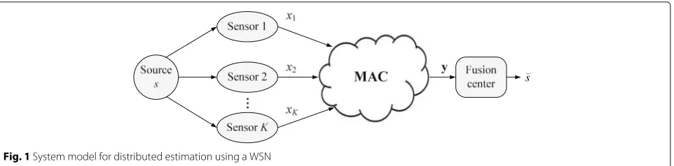
Figure 1 shows a system model of distributed estimation using a WSN. Here, a scalar Gaussian random variable sis observed in a memoryless fashion byK sensors and each observation is subject to white Gaussian noise. The observation of theith sensor can be expressed as
xi =s+vi, 1≤i≤K, (1)
where the source signal s and observation noise vi are
treated as random variables with zero mean and variances
σ2
s andσv2, respectively. The observation signal-to-noise
ratio (SNR) is defined asγo= σ 2
s σ2
v.
Using analog modulation, theith sensor simply ampli-fies xi with a gain ai and transmits the result to the
FC. The total transmit power in this WSN is Ptot =
K i=1a2i
σ2 s +σv2
. The communication channels from sensors to the FC are considered to be wireless fading channels. Let hi = riejϕi, i = 1,. . .,K, represent the
s
Fig. 1System model for distributed estimation using a WSN
responses are modeled as independent and identically dis-tributed (i.i.d.) complex Gaussian random variables with zero mean and unit variance, denoted as CN(0, 1). This also means that the magnituderi and phaseϕiare
inde-pendent random variables with Rayleigh and uniform distributions, respectively. On each wireless fading chan-nel, the transmitted signal is disturbed by additive white Gaussian noise (AWGN). The AWGN sample, denoted as
ω, is modeled as a complex Gaussian random variable with zero mean and varianceσω2. ThechannelSNR is defined asγc= Pσtotω2 .
The received signal at the FC is generally denoted by y = y1,y2,. . .,yN. The dimension N and expression
of y in terms ofai, xi, hi and ωdepend on the type of
multiple access channel (MAC) realized from the sensors to the FC. This is elaborated in the below subsections. Regardless of the type of MAC, the task of the FC is to estimate the underlying source signal based on the received signaly. Using the linear minimum mean square error (LMMSE) estimator [27] and assuming that all the channel responses are available at the FC, the estima-tion of s is ˇs = CsyC−yy1y, whereCsy is the covariance betweensandyandCyyis the covariance ofy. The cor-responding MSE is = σs2−CsyC−yy1Cys, which depends
on the specific realizations of channel responses hi’s.
The long-term performance of a WSN is evaluated using
the average MSE (AMSE), defined as AMSE = E{},
where the expectation is taken over channel response realizations.
2.1 Coherent MAC
With the coherent MAC [8], after the phases of chan-nel responses are compensated at sensors, signals from all sensors are essentially transmitted on one (equivalent)
channel. Thus, the dimension of y is N = 1, i.e., the
received signal at FC is a scalar. To realize phase compen-sation at the transmitters, the phase values of the wireless channel responses need to be sent from the FC to all sen-sors, which represents a large amount of feedback. After phase compensation, the transmitted signal at theith sen-sor isxi= ai(s+vi)e−jϕi. Under timing synchronization
among the sensors, all the useful information resides in
the real part of the received signal at the FC, which can be expressed as4
y= K
i=1
ai(s+vi)ri+R{ω}. (2)
The LMMSE estimator and the corresponding MSE are given as
ˇ
scoh= ⎡ ⎢ ⎣
K
i=1airi
σ2 s
K
i=1airi 2
σ2 s +
K
i=1a2iri2
σ2 v +σ
2
ω 2
⎤ ⎥ ⎦y,
(3)
coh= ⎡ ⎢ ⎣σ−2
s +
K
i=1airi 2
K
i=1a2iri2
σ2 v +
σ2
ω 2
⎤ ⎥ ⎦
−1
. (4)
2.2 Orthogonal MAC
With the orthogonal MAC [7],K sensors transmit their
observations to the FC via K orthogonal channels. The
orthogonal MAC does not require feedback of channel responses from the FC to the sensors, and hence is more favorable for implementation. However, the key disadvan-tage of the orthogonal MAC is that it requires a larger transmission bandwidth or longer latency to realize mul-tiple orthogonal channels. At the FC, the channel phase on each wireless channel is compensated first. After such phase compensation, all the useful information is found in the real parts of the processed signals. On theith wireless channel, by taking the real part of the complex baseband signal, one has
yi=ai(s+vi)ri+R
ωe−jϕi =airis+aiviri+R
ωe−jϕi= ¯r
is+ ¯vi+ ¯ωi,
(5)
wherer¯i=airi,v¯i=aiviriandω¯i=Rωe−jϕi.
Let y = y1,y2,. . .,yK
, ¯r = [r¯1,r¯2,. . .,r¯K], v¯ =
turns toy= ¯rs+ ¯v+ ¯ω. It then follows that the LMMSE estimator ofsbased onyis
ˇ
The corresponding MSE distortion is
orth=
2.3 Hybrid MAC
With the hybrid MAC considered in [17], all sensors are divided into groups and the coherent MAC is used for sen-sors within each group, whereas the orthogonal MAC is used across different groups. This MAC provides a
solu-tion for scenarios where there are N (a small number
due to bandwidth constraint) orthogonal channels that are shared byKsensors, whereK ≥N. In this hybrid MAC, to obtain coherent combination in each group, channel phase information feedback from the FC to the sensors is still required and the amount of feedback is the same as that of the coherent MAC. In addition, the required trans-mission bandwidth in this MAC depends on the number of sensor groups.
After phase compensation, the transmitted signal at the ith sensor isxi = ai(s+vi)e−jϕi. Under timing
synchro-nization among the sensors in the same group, on the nth equivalent channel, all the useful information is in the real part of the received signal at the FC, which can be expressed as
to the orthogonal MAC, the LMMSE estimator ofsbased
onyis
andω¯ is still the same as (8). The corresponding MSE distortion is
2.4 Semi-orthogonal MAC
The semi-orthogonal MAC can be considered as a direct competitor of the hybrid MAC in the sense that they are both suitable for the scenarios where there areN orthog-onal channels that are shared byKsensors, whereK≥N. The key novelty in realizing the semi-orthogonal MAC is that theith sensor transmits to the FC according to a length-Nvectorg(i) =
g1(i),g2(i),. . .,gN(i)
, whose element
is either 0 or 1. The set ofg(i)’s gives an allocation ofN orthogonal channels toK sensors. For theith sensor, if thenth element ofg(i) is 1, then theith sensor transmits on thenth orthogonal channel.5Under timing synchro-nization among the sensors, the received signal on thenth orthogonal channel at the FC is
yn= Equation (14) can be rewritten as
yn=
defined as the equivalent channel response and
of the equivalent channel responsehˆnis compensated to
The above phase compensation discards halves of obser-vation noise and channel noise. It is pointed out that the phase compensation of the equivalent channel response is performed at the FC. Therefore, no phase information is needed at the sensors and feedback of channel phase information is not required.
Lety¯ = y¯1,y¯2,. . .,y¯N
andω¯ is still the same as (8). The corresponding MSE distortion is
The above expression clearly shows that the estima-tion performance under a semi-orthogonal MAC strongly
depends on howN orthogonal channels are shared byK
sensors, i.e., how the sensors are grouped. The two sensor
grouping strategies proposed in the next section are based on the two performance indicators established as follows. First, settingσv2=0 givesv¯=0and the MSE distortion
The parameter α indicates the impact of channel noise
on the MSE performance. The largerα is, the lesser the impact is.
On the other hand, settingσω2=0 givesω¯ =0and the MSE distortion is
semi−β= In this case, the parameterβindicates the impact of obser-vation noise on the MSE performance. The largerβis, the lesser the impact is.
3 Sensor grouping methods for semi-orthogonal MAC
3.1 Fixed sensor grouping
Fixed sensor grouping means that the assignment of orthogonal channels, once decided, does not change
dur-ing the communication phase. When assigndur-ingN
orthog-onal channels toK sensors, whereK ≥ N, an obvious
question arises:Should more than one orthogonal channel be assigned to a single sensor and will this improve the MSE performance of distributed estimation?
To answer the above question, let us first examine a simple scenario where there are two orthogonal channels (N = 2) withK1sensors transmitting on each of them. Under equal power allocation, the gain factor isai= ¯a=
* P
sensors that transmit on both orthogonal channels.
Treat-ing the equivalent channel responseshˆ1= ¯a K
g2(i)hias random variables, the correlation
groups with sensors in each group transmitting on one orthogonal channel.
Next, define h˜1 = √21K 1
K
i=1g(1i)hi and h˜2 = 1
√
2K1 K
i=1g (i)
2 hi, which are basically the scaled versions
of h¯1 and h¯2 defined in (16). Then, the parameterα is
α = |˜h1|2+ |˜h2|2. Since each of h˜1 andh˜2is a 1/√2K1 times the sum ofK1i.i.d. complex Gaussian random vari-ables, each with zero mean and unit variance, it is a complex Gaussian random variable with zero mean and variance 1/2. It follows immediately that the expected value of α is E{α} = 1. To find the expression for β, expressh˜1andh˜2ash˜1= m√12ejφ1 andh˜2= √m22ejφ2. Then, Appendix A shows that, whenKapproaches infinity,β =
2m2
1−2ρcos(φ1−φ2)m1m2+m22
1−ρ2cos2(φ1−φ2) . The expectation ofβis more tedious to obtain, and it is given in (61) of Appendix A.
Table 1 tabulates the values ofE{β}versusρ, obtained by theory and simulation. The theoretical and simulation results match very well. As can be seen, whileE{α}is a constant 1,E{β}is a monotonically-decreasing function of ρ. This means that, while the correlation among the equivalent channel responses does not affect the chan-nel noise suppression capability, it reduces the observa-tion noise suppression capability. Overall, the correlaobserva-tion among the equivalent channel responses degrades the estimation performance, and hence should be avoided. This can be done by not assigning more than one orthog-onal channel to each sensor.
ForN >2, it is not easy to determine channel allocation among sensors and perform the corresponding correla-tion analysis among the equivalent channel responses of the orthogonal channels. Instead, the following example of ad hoc channel allocation scheme shall be investigated. Assume thatKis an integer multiple ofN. If(n−N1)K+K1≤ K, then thenth orthogonal channel is shared by sensors with indices in the set of
(n−1)K
N +1,. . .,( n−1)K
N +K1
.
If (n−N1)K + K1 > K, then the set of sensor indices is
1,. . .,(n−N1)K +K1−K
∪(n−1)K
N +1,. . .,K
. With
such a channel assignment, as long as K1 > KN, some sensors will transmit on more than one orthogonal chan-nel and the correlation among the equivalent chanchan-nel
responses of orthogonal channels is not zero. As K1
increases from NK toK, more and more sensors transmit on more than one orthogonal channel and the correlation among the equivalent channel responses increases from 0
to 1. Therefore,K1can be adjusted for different levels of correlation among the equivalent channel responses.
With the above channel allocation scheme, the
param-eter α defined in (22) can be expressed as α =
1 N
N
n=1|˜hn|2, whereh˜nis√1K
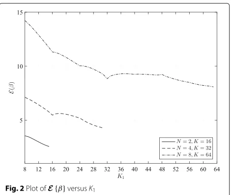
1 of the sum ofK1i.i.d. zero-mean unit-variance complex Gaussian random variables. It then follows that the expected value ofαalso equals to 1 in this case. Since the analytical expression ofE{β}is not available, simulation results are obtained and shown in Fig. 2 for three settings of (N =2,K =16), (N =4,K = 32) and (N = 8,K = 64). In obtaining these simulation results, the power allocation is performed such that each sensor transmission on one orthogonal channelconsumes the same power ofPtot/(NK1). It is observed from Fig. 2 that asK1 increases,E{β}generally decreases, although not monotonically. The non-monotonic decrease ofE{β} versus increasingK1is due to the ad hoc channel assign-ment and power allocation described above. In particular, the adopted power allocation is quite “non-uniform” in the sense that the total power allocated to a given sen-sor is proportional to the number of orthogonal channels assigned to it. Depending onK1, this number ranges from 1 toN for each sensor, whereas a larger K1 reduces the power levelPtot/(NK1)allocated for each sensor transmis-sion. The most important observation of this figure is that
E{β}takes on the largest value whenK1= KN as expected. From the above theoretical derivations and simulation results, it can be concluded that only one orthogonal channel should be assigned to each sensor. In other words, all sensors are divided into disjoint groups and those sen-sors in the same group transmit on one orthogonal channel. Moreover, the fixed sensor grouping proposed here is such that all sensors are equally divided into groups, i.e., thenth group isn=
(n−1)K
N +1,. . ., nK
N
.
3.2 Adaptive sensor grouping
With the fixed sensor grouping described in the previous subsection, the parameterαcan be written as
α=
N
n=1
i√∈nhi K
2 # $% &
αn =
N
n=1
αn, (25)
where eachαn is affected only by the channel responses
of sensors transmitting on the nth orthogonal channel. Therefore αn can be interpreted as an indicator of the
Table 1Values ofE{β}withN=2
ρ 0.05 0.1 0.2 0.3 0.4 0.5 0.6 0.7 0.8 0.9 0.95
Theory 3.984 3.969 3.909 3.812 3.680 3.518 3.333 3.133 2.930 2.741 2.655
Fig. 2Plot ofE{β}versusK1
channel noise suppression capability of thenth orthogonal channel. Similarly, the parameterβcan be expressed as
β=
N
n=1
i∈ naihi
2
i∈na
2 i
R{hi}
Rhnˆ
hnˆ +I{hi}
Ihnˆ hnˆ
2
# $% &
βn
= N
n=1
βn,
(26)
where βn is also affected only by the channel responses
of sensors transmitting on the nth orthogonal channel, and it can be interpreted as the indicator of the obser-vation noise suppression capability of thenth orthogonal channel.
The above simple observation suggests that if all sen-sors can be properly grouped according to their channel responses, larger αn and βn can be obtained for each
orthogonal channel and thus the overall channel noise suppression and observation noise suppression capabili-ties of the semi-orthogonal MAC will be improved.
Intuitively, sensors with channel responses of similar phases should be grouped together to get better channel noise suppression and observation noise suppression. Will this “similar phase” grouping strategy work and how to define “similar phase”? To answer this question, examine a scenario that one sensor with channel response of mag-nitude 1 and phase 0 transmits on an orthogonal channel. Both the indicators of the channel noise suppression and observation noise suppression of this orthogonal channel are 1. Next, add another sensor with channel response of magnitude r(r < 1) and phase ϑ (0 ≤ ϑ ≤ π) to
form a group7. Then the two indicators of this orthogonal channel change to:
αn=(rcosϑ+1)2+(rsinϑ)2=r2+2rcosϑ+1,
(27)
βn=
r2+2rcosϑ+1
(cosφ)2+(rcosϑcosφ+rsinϑsinφ)2, (28) whereφ is the phase of the equivalent channel response and tanφ= rcosrsinϑϑ+1.
If αn > 1, the added sensor is said to beconstructive
for channel noise suppression and ifβn > 1, the added
sensor is constructivefor observation noise suppression. Note that if the added sensor transmits on an orthogo-nal channel alone, thenαn = r2andβn = 1. This means
that if the added sensor is constructive, sensor grouping improves performance of individual sensors (i.e., without being grouped).
To determine if the added sensor is constructive for channel noise suppression and/or observation noise sup-pression, it is straightforward to show from (27) and (28) that
+
αn>1, if 0≤ϑ <arccos−r2
αn≤1, if arccos
−r 2
≤ϑ≤π (29)
+
βn>1, if 0≤ϑ <arccos(−r)
βn≤1, if arccos(−r)≤ϑ≤π (30)
The above analysis leads to the following three regions ofϑ:
• Ifϑis in region A, i.e.,0≤ϑ <arccos−2r, the added sensor is constructive for both channel noise suppression and observation noise suppression. Note that region A includes0,π2, regardless of the value ofr.
• Ifϑis in region B, i.e.,
arccos−2r≤ϑ <arccos(−r), the added sensor is destructive for channel noise suppression, but constructive for observation noise suppression.
• Ifϑis in region C, i.e.,arccos(−r)≤ϑ < π, the added sensor is destructive for both channel noise suppression and observation noise suppression.
At this point, the question raised at the beginning of this section has been answered for grouping two sensors. In summary, if the phase difference between the channel responses of the two sensors is in the region of0,π2, sen-sor grouping is beneficial. However, if the phase difference is larger thanπ2, grouping sensors on the same orthogonal channel may be destructive for either channel noise sup-pression or observation noise supsup-pression, or for both of them, and sensor grouping may give worse performance. Therefore, if the semi-orthogonal MAC is employed with
is partitioned into N = 2 orN = 3 equal sub-regions (each of lengthπor 2π/3), then grouping the sensors with channel phases in the same sub-region to transmit on the same orthogonal channel might not always be beneficial. However, if the semi-orthogonal MAC is used withN≥4 and the whole phase region is partitioned intoN equal sub-regions (each of length 2Nπ), then grouping the sen-sors with channel phases in the same sub-region always picks constructive sensors in one group and therefore performance improvement is guaranteed8.
In summary, for N ≥ 4, adaptive sensor grouping
is always beneficial and is done such that all sensors
whose channel phases fall into the same nth region
2π(n−1)
N ,2Nπn
transmit on the nth orthogonal channel. This adaptive sensor grouping is analyzed in more detail in the next section.
4 Performance analysis
In general, with the same number of sensors, different MACs yield different values of E(α) and E(β), imply-ing different capabilities of channel noise suppression and observation noise suppression. This section analyzes in detail the estimation performance of the semi-orthogonal MAC under fixed and adaptive sensor grouping and also compare with the coherent MAC, orthogonal MAC and hybrid MAC. The analysis and comparison are car-ried out for equal power allocation, i.e., ai = ¯a =
4.1 Orthogonal, coherent, and hybrid MACs
Under equal power allocation, the MMSE distortions obtained with the LMMSE estimator for the orthogonal, coherent, and hybrid MACs can be shown to be:
orth=
For the orthogonal MAC, it is easily seen that
Eorth(α)=EKi=1|hi|
K is a Gaussian
random variable with mean √KE(|hi|) and variation
, it follows that
E(|hi|)=
Similarly, it can be shown for the hybrid MAC that
Ehyb(α) = E
4.2 Semi-orthogonal MAC with fixed sensor grouping
For the parameter α, one has Esemi−F{α} = case of the orthogonal MAC.
The expected value ofβ is difficult to obtain for arbi-trary values ofKandN. To gain some insight, the pdf of
βis obtained by simulation and plotted in Fig. 3 for vari-ous values of NK. The corresponding values ofEsemi−F{β} are shown in Table 2. Figure 3 clearly shows that, as long asKN >1, there is a high probability that the value ofβis larger thanN =4. Furthermore, the larger the ratio KN is, the more likelyβtakes on a larger value.
WhenK → ∞, it is shown in Appendix B that that
β follows a Gamma distribution with parametersa= N
Fig. 3Pdf of parameterβwithN=4
4.3 Semi-orthogonal MAC with adaptive sensor grouping As discussed in Section 3.2, adaptive sensor grouping is
beneficial whenN ≥ 4. To implement the adaptive
sen-sor grouping, thenth sub-region of the phase partition is [ϑ1,ϑ2), whereϑ1= 2π(Nn−1)andϑ2= 2πNn. Lethi=x+jy
and focus on the case that the phase ofhifalls into the first
sub-region [ 0, 2π/N). With N equal-length sub-regions of the phase, the probability that the phase of a channel response falls into a specific sub-region is 1/N. Thus, the joint pdf ofxandyis simply
means and variances ofxandyare
μx=
yn are i.i.d Gaussian random variables with means and
variances It then follows that
E{αn} =Ex˜2n+ ˜y2n
On the other hand,
E{βn}
2 andκtakes on the following value:
5 Numerical results and discussions
Table 3 comparesE{α}andE{β}among different MACs
for a fixed number of sensors, K. To put these
num-bers in perspective, the number of orthogonal channels,
N, and the amount of feedback required by each type
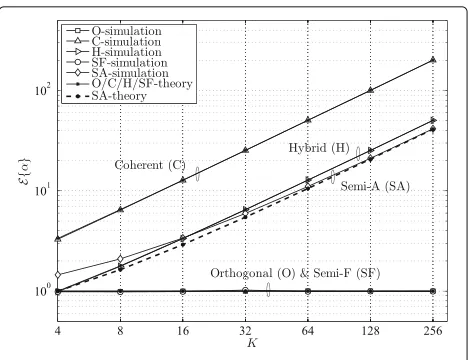
of MAC are also indicated in the table. The theoretical and simulation results ofE{α} and E{β} are plotted in Figs. 4 and 5, respectively. Observe that whenK is large enough, the theoretical results agree very well with the simulation results. For smallK, the simulation result is better than the theoretical result for E{α} of the semi-orthogonal MAC with fixed sensor grouping. As forE{β}, there are differences between the theoretical and simula-tion results of the hybrid MAC, and the semi-orthogonal MAC (with either fixed or adaptive sensor grouping). This observation suggests that for these three MACs, a suffi-ciently large number of sensors is required to achieve the asymptotic performance.
For the semi-orthogonal MAC with adaptive sensor grouping andN=4, asK→ ∞,E{α}andE{β}increases in the order ofK, and thus the average MSE distortion goes to zero. This phenomenon is the same as those of both the coherent and hybrid MACs. However, for the orthogo-nal MAC and the semi-orthogoorthogo-nal MAC with fixed sensor grouping, the average MSE distortion converges to a fixed value asKincreases. This is becauseE{α} =1, regardless ofK, for these two MACs.
The semi-orthogonal MAC with adaptive sensor group-ing can achieve the same performance at lowγcand even better performance at highγcas compared to the coher-ent MAC. However, the semi-orthogonal MAC requires
N = 4 times the number of orthogonal channels and
about five times the number of sensors. Nevertheless, it does not require channel phase information feedback. Furthermore, the semi-orthogonal MAC with adaptive sensor grouping can performs very close to the hybrid MAC. According to the simulation results in Fig. 4, for
E{α}, the semi-orthogonal MAC is better for smallKbut worse for largeK. With aboutK=16, the two MACs have the sameE{α}. ForE{β}, the semi-orthogonal MAC per-forms nearly the same as the hybrid MAC for all values of K. Again, it is important to point out that channel phase information feedback is needed in the hybrid MAC.
Fig. 4Simulation and theoretical results ofE{α}
It is of interest to investigate the impact of the num-ber of orthogonal channels N on the estimation perfor-mance under the semi-orthogonal MAC with adaptive sensor grouping. To this end, the theoretical quantities
E{α}
K and E
{β}
K are plotted versus N for a sufficient large K (K = 128N) in Fig. 6, where the simulation results are also provided to verify the theoretical derivations. As can be seen, as N increases from 4, E{Kα} decreases while E{Kβ} stays nearly the same. Therefore with a fixed K, ifNincreases, which means more orthogonal channels and each with fewer sensors transmitting on, the channel noise suppression capability degrades, while the observa-tion noise suppression capability is practically unchanged. The degradation of the channel noise suppression capabil-ity due to having more orthogonal channels is reasonable, because with more orthogonal channels, the FC needs to collect and process a larger number of received sig-nal samples that are disturbed by independent AWGN noise components, resulting in a larger noise power over-all. On the other hand, the observation noise suppression capability is determined only by the number of sensors, independent of the number of orthogonal channels.
It is pointed out that Fig. 6 also provides the results
for N = 2. Compared to N = 4, although there are
fewer orthogonal channels and thus smaller (overall) noise
Table 3Asymptotic performance in terms ofE{α}andE{β}
Type of MAC E{α} E{β} Number of orthogonal
channels,N
Required feedback
Coherent 0.78K 0.78K 1 Exact channel phase
Orthogonal 1 K K None
Hybrid (N=4) 0.20K 0.78K 4 Exact channel phase
Semi-orthogonal, fixed (N=4) 1 8 4 None
Fig. 5Simulation and theoretical results ofE{β}
power for N = 2, usingN = 2 has almost the same
channel noise suppression capability as using N = 4.
In addition, the observation noise suppression
capabil-ity for N = 2 is much weaker than that for N = 4.
These phenomenons are consistent with the analysis in
Section 3.2. In general, N = 4 is the best choice for
the semi-orthogonal MAC with adaptive sensor group-ing, which achieves the largest performance improvement while requiring the least transmission bandwidth.
The qualitiesEK{α}and E{Kβ} are also plotted in Fig. 6 for the hybrid MAC. The advantage of the hybrid MAC over the semi-orthogonal MAC with adaptive sensor
group-ing is most obvious for N = 2. Again, this is because
with N = 2, destructive superposition of signals from
two sensors happens in the semi-orthogonal MAC, while it is never the case in the hybrid MAC. AsN increases, the sub-regions of channel phases become narrow, and the direct superposition behaves more and more like the
coherent combination. ForN = 8, the two MACs have
nearly the same performance.
Fig. 6Plots ofE{Kα}andE{Kβ}, by simulation and theoretical analysis
Regarding the bandwidth requirement (in terms of the number of orthogonal channels), the hybrid and semi-orthogonal MACs are much more efficient than the orthogonal MAC. The coherent MAC is the most band-width efficient since only one channel is used. For the orthogonal MAC and the semi-orthogonal MAC with fixed sensor grouping, no feedback of channel phases from the FC to the sensors is required. For the coherent MAC, due to the requirement of coherent combination among sensors, channel phases need to be transmitted from the FC to the sensors. The exact number of bits used for such information feedback depends on the capability of the feedback channel and the required accuracy, but this is certainly a large amount of overhead. For the hybrid MAC, because coherent combination among sensors in each group is required, the amount of channel informa-tion feedback from the FC to the sensors is still the same as that of the coherent MAC. For the semi-orthogonal MAC with adaptive sensor grouping, the FC needs to send only log2Nbits to inform each sensor the orthogonal channel to transmit on.
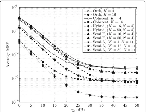
The simulation results of average MSE achieved by the five MACs under comparison are plotted in Fig. 7. When
K = N = 4, the coherent MAC obviously outperforms
the other 4 MACs at lowγc, which is due to its outstand-ing capability on channel noise suppression. In this case, the hybrid MAC and the semi-orthogonal MAC with fixed sensor grouping are equivalent to the orthogonal MAC. The semi-orthogonal MAC with adaptive sensor grouping performs a little better than the orthogonal MAC.
With K increasing from K = 4 to K = 16, the
per-formance improvements are significant, except for the semi-orthogonal MAC with fixed sensor grouping. In
particular, the performance of the semi-orthogonal MAC with adaptive sensor grouping is the same as that of the hybrid MAC, which is consistent with the theoretical derivation, and it is between those of the orthogonal MAC and the coherent MAC.
WhenK is further increased to K = 80, the
perfor-mance of the semi-orthogonal MAC with fixed sensor grouping stays nearly the same as the performance with K=16. On the other hand, the performance of the semi-orthogonal MAC with adaptive sensor grouping improves significantly. The semi-orthogonal MAC with adaptive sensor grouping andK =80 achieves the same (at lowγc) or even better (at highγc) performance compared to the
coherent MAC with K = 16. In addition, with K =
80, the hybrid MAC only slightly outperforms the semi-orthogonal MAC at low γc. All the simulation results match with the theoretical analysis presented before.
Finally, the average MSE performances of the semi-orthogonal MAC with adaptive sensor grouping are com-pared forN=4 andN=8. As shown in Fig. 8, at lowγc, for the network withK=80, usingN=8 cannot achieve the same performance as usingN = 4. IfK increases to 140 forN = 8, then the performance is the same as that
of having N = 4 andK = 80. This is consistent with
the previous theoretical and simulation results, which are E{α}
K ≈0.16 forN=4 andE{Kα} ≈0.094 forN=8. 6 Conclusions
For WSNs consisting of a sufficient large number of sen-sors but operating under limited bandwidth resource, a novel semi-orthogonal multiple access scheme was
pro-posed for transmission from K sensors to the FC over
N orthogonal channels, whereK ≥ N. The paper
thor-oughly analyzed the performance of distributed estima-tion over such a semi-orthogonal MAC with either fixed
Fig. 8Performance comparison in terms of the average MSE forN>4
or adaptive sensor grouping and compared with the
performance achieved with other related MACs. Com-pared to the orthogonal MAC operating under the same bandwidth, the semi-orthogonal MAC with fixed sensor grouping has the same channel noise suppression capabil-ity, but twice the observation noise suppression capability asKapproaches infinity. This is achieved with no require-ment of information feedback from the FC to sensors. For the semi-orthogonal MAC with adaptive sensor grouping, it is determined thatN = 4 is the most favorable num-ber of orthogonal channels when taking into account both performance and feedback requirement. In particular, the semi-orthogonal MAC with adaptive sensor grouping is shown to perform very close to that of the hybrid MAC under the same bandwidth and number of sensors, while requiring only two bits of information feedback instead of the exact channel phase for each sensor.
The present paper considers estimating a single source signal. In general, when the number of sources increases, the amount of information to transmit from the sensors to the FC increases, which translates to a larger transmission bandwidth, or equivalently a larger number of orthogo-nal channels. If the sources are uncorrelated, the proposed semi-orthogonal transmission framework can be applied individually for each source signal. However, if the source signals are correlated, the correlation information should be used in the development of joint semi-orthogonal mul-tiple access schemes and this is left for further research.
Endnotes
1To be consistent with existing literature, the term MAC
is also used in this paper, although it is more appropriate to use the term “multiple access scheme” when discussing different communication methods between the sensors and FC.
2The definition and meaning of equivalent channel
responses will be made clearer in Section 3.
3The interested reader is referred to [28] for a novel
power allocation solution under the semi-orthogonal MAC, which is shown to improve the estimation perfor-mance when compared to equal power allocation, espe-cially at low channel signal-to-noise ratios.
4For complex scalars, vectors and matrices, R{·}
denotes the real part andI{·}denotes the imaginary part.
5This allocation is similar to the transmission in an
overloaded code-division multiple access (CDMA) sys-tems [29, 30] if one views vector g(i) as the signature vector of sensori.
6For random variables,E{·}andD{·}denote
7If the channel response of the added sensor is of
mag-nitude larger than 1, then it can be taken as the first sensor and the other sensor is taken as the added sensor.
8Since the phases of wireless channel responses are
modeled as uniform, one does not expect any benefit to use non-uniform phase partitions.
Appendix A
To obtain the expression forβ, first one has (recall (18) for the definition ofθn,l)
When K and K1 approach infinity, one has
K It then follows that
θ1,2= σ
. According to the central limit theorem,
m1ejφ1andm2ejφ2are two complex Gaussian random vari-ables with zero mean and unit variance. Furthermore, the
correlation coefficient between m1ejφ1 and m2ejφ2 is ρ.
It then follows that
Next,
gamma functions [31]. Since x
are odd functions ofxand the integral with respect toxis from−1 to 1, the two terms integrate to zero. Then one has
+ (x,m2)
One also can compute
4 ∞
Under equal power allocation, the expression of βn for
the semi-orthogonal MAC with fixed sensor grouping simplifies to
larly symmetric complex Gaussian random variables with zero mean and variance 1. The numerator ofβn,|˜hn|2, is
of exponential distribution with parameterλ = 1, whose pdf is
numbers, (64) turns to
Therefore, whenK → ∞,βn =2|˜hn|2is exponentially
distributed with parameterλ=2, whose pdf is
fβn(βn)=
1 2exp
β n
2
, βn≥0. (66)
Finally, it is well known that the sum of N indepen-dent and iindepen-dentically distributed (i.i.d.) exponential
ran-dom variables with parameterλ=2 is a Gamma random
variable with parametersa = N andb = 2. For
com-pleteness, the pdf of the Gamma distribution is as follows:
fβ(β)= β a−1
(a)baexp
−β
b
, β ≥0, a>0, b>0,
(67)
where (a)=50∞xa−1e−xdxis the Gamma function. Ifa is an integer, then (a)=(a−1)!.
Acknowledgements
This work was supported by a Discovery Grant from the Natural Sciences and Engineering Council of Canada (NSERC). The authors would like to thank the anonymous reviewers for many constructive comments, which greatly helped in improving the clarity of this paper.
Authors’ contributions
The work was carried out by the first author when she was a graduate student under the academic supervision of the second author. Both authors read and approved the final manuscript.
Competing interests
The authors declare that they have no competing interests.
Received: 23 February 2016 Accepted: 27 August 2016
References
1. IF Akyildiz, W Su, Y Sankarasubramaniam, E Cayirci, A survey on sensor networks. IEEE Commun. Mag.40, 102–114 (2002)
2. VC Gungor, GP Hancke, Industrial wireless sensor networks: challenges, design principles, and technical approaches. IEEE Trans. Ind. Electron.56, 4258–4265 (2009)
3. VC Gungor, B Lu, GP Hancke, Opportunities and challenges of wireless sensor networks in smart grid. IEEE Trans. Ind. Electron.57, 3557–3564 (2010)
4. C-Y Chong, SP Kumar, Sensor networks: evolution, opportunities and challenges. Proc. IEEE.91, 1247–1256 (2003)
5. M Nourian, S Dey, A Ahlen, Distortion minimization in multi-sensor estimation with energy harvesting. IEEE J. Select. Areas in Commun.33(3), 524–539 (2015)
6. J-J Xiao, A Ribeiro, Z-Q Luo, G Giannakis, Distributed
compression-estimation using wireless sensor networks. IEEE Signal Proc. Mag.23, 27–41 (2006)
7. S Cui, JJ Xiao, ZQ Luo, A Goldsmith, HV Poor, Estimation diversity and energy efficiency in distributed sensing. IEEE Trans. Signal Process.55, 4683–4695 (2007)
8. JJ Xiao, S Cui, ZQ Luo, A Goldsmith, Linear coherent decentralized estimation. IEEE Trans. Signal Process.56, 757–770 (2008) 9. M Gastpar, M Vetterli, inLecture Notes in Computer Science.
Source-channel communication in sensor networks, vol. 2634 (Springer, New York, 2003), pp. 162–177
10. M Gastpar, Uncoded transmission is exactly optimal for a simple Gaussian “sensor” network. IEEE Trans. Inform. Theory.54, 5247–5251 (2008) 11. K Liu, H El-Gamal, A Sayeed, inIEEE/SP 13th Workshop on Statist. Singal
Process. On optimal parametric field estimation in sensor networks
(IEEE/SP 13thWorkshop on Statist. Singal Process, Bordeaux, 2005), pp. 1170–1175
12. W Bajwa, A Sayeed, R Nowak, in4th Int. Symp. Inf. Process. Sens. Netw. Matched source-channel communication for field estimation in wireless sensor network, (Los Angeles, 2005), pp. 332–339
13. MK Banavar, C Tepedelenlioglu, A Spanias, Estimation over fading channels with limited feedback using distributed sensing. IEEE Trans. Signal Process.58, 414–425 (2010)
14. H Senolm, C Tepedelenlioglu, Performance of distributed estimation over unknown parallel fading channels. IEEE Trans. Signal Process.56, 6057–6068 (2008)
15. TJ Goblick, Theoretical limitation on the transmission of data from analog sources. IEEE Trans. Inform. Theory.IT-11, 558–567 (1965)
16. M Gastpar, B Rimoldi, M Vetterli, To code or not to code: lossy source-channel communication revisited. IEEE Trans. Inform. Theory.49, 1147–1158 (2003)
17. JC Liu, CD Chung, Distributed estimation in a wireless sensor network using hybrid mac. IEEE Trans. Veh. Technol.60, 3424–3435 (2011) 18. R Mudumbai, G Barriac, U Madhow, On the feasibility of distributed
beamforming in wireless networks. IEEE Trans. Wireless Commun.6, 1754–1763 (2007)
19. C Tepedelenlioglu, On the asymptotic efficiency of distributed estimation systems with constant modulus signals over multiple-access channels. IEEE Trans. Inform. Theory.57, 7125–7130 (2011)
20. M Gastpar, M Vetterli, Power, spatio-temporal bandwidth, and distortion in large sensor networks. IEEE Trans. Inform. Theory.23, 745–754 (2005) 21. Su J, Distributed estimation in wireless sensor networks under
semi-orthogonal MAC. M.Sc. Thesis, University of Saskatchewan, Canada, 2014
22. I Bahceci, AK Khandani, Linear estimation of correlated data in wireless sensor networks with optimum power allocation and analog modulation.
56, 1146–1156 (2008)
23. J-Y Wu, T-Y Wang, Power allocation for robust distributed bestlinear-unbiased estimation against sensing noise variance uncertainty. IEEE Trans. Wireless Commun.12, 2853–2869 (2013)
24. S Kar, PK Varshney, Linear coherent estimation with spatial collaboration. IEEE Trans. Inform. Theory.59, 3532–3553 (2013)
25. J Fang, H Li, Power constrained distributed estimation with cluster-based sensor collaboration. IEEE Trans. Wireless Commun.8, 3822–3832 (2009) 26. M Fanaei, MC Valenti, A Jamalipour, NA Schmid, inProc. IEEE Acoustics,
Speech and Signal Process. Optimal power allocation for distributed BLUE estimation with linear spatial collaboration, (Florence, 2014),
pp. 5452–5456
27. SM Kay,Fundamentals of statistical signal processing: estimation theory. (Prentice-Hall, Inc., Englewood Cliffs, 1993)
28. J Su, HH Nguyen, HD Tuan, inCanadian Workshop on Information Theory. Power allocation for distributed estimation in sensor networks with semi-orthogonal MAC, (St. John’s, 2015)
29. VAP Viswanath, DNC Tse, Optimal sequences, power control and user capacity of synchronous CDMA systems with linear MMSE multiuser receiver. IEEE Trans. Inform. Theory.45, 1968–1983 (1999)
30. HH Nguyen, E Shwedyk, Bandwidth constrained signature waveforms for maximizing the network capacity of synchronous CDMA systems. IEEE Trans. Commun.49, 961–965 (2001)