A new parallel algorithm for solving parabolic equations

R E S E A R C H

Open Access

A new parallel algorithm for solving

parabolic equations

Guanyu Xue

_{and Hui Feng}

*_{Correspondence:} [email protected] 1_{School of Mathematics and} Statistics, Wuhan University, Wuhan, China

Abstract

In this paper, a new parallel algorithm for solving parabolic equations is proposed. The new algorithm includes two domain decomposition methods, each method is applied to compute the values at (n+ 1)st time level by use of known numerical solutions atnth time level, respectively. Then the average of two above values is chosen to be the numerical solutions at (n+ 1)st time level. The new algorithm obtains satisfactory accuracy while maintaining parallelism and unconditional stability. This algorithm can be extended to solve two-dimensional parabolic equations by alternating direction implicit (ADI) technique. Both error analysis and numerical experiments illustrate the accuracy and efficiency of the new algorithm.

Keywords: Parabolic equations; Finite difference; Unconditional stability; Parallelism

1 Introduction

With the development of large-scale scientific and engineering computations, the paral-lel difference method for parabolic equations has been studied rapidly. In 1983, Evans and Abdullah [1] proposed the Group Explicit (GE) scheme for solving the parabolic equations by Saul’yev asymmetric schemes [2]. Evans [3] first constructed the Alternating Group Ex-plicit (AGE) scheme for the diffusion equation two years later. The Alternating Segment Explicit–Implicit (ASE-I) scheme and the Alternating Segment Crank–Nicolson (ASC-N) scheme were designed in [4–6]. Afterwards, the alternating segment algorithms (AGE scheme, ASE-I scheme, and ASC-N scheme) above became very effective methods for some parabolic equations, such as heat equation [7], convection–diffusion equation [8– 10], dispersive equation [11–16], forth-order parabolic equation [17–19]. Meanwhile, do-main decomposition methods (DDMs) for the partial differential equations have been studied extensively [20–29]. The concept called “intrinsic parallelism” was presented in [30–32]. In 1999, the alternating difference schemes were presented, the unconditional stability analysis was given in [33]. The unconditionally stable domain decomposition method was obtained by the alternating technique in [34–36]. In fact, an alternating seg-ment algorithm is also a form of the domain decomposition method, which is not only suitable for parallel computation but also unconditionally stable. However, the accuracy of alternating segment algorithm is unsatisfactory.

Inspired by the alternating segment algorithm, we present a new parallel algorithm for parabolic equations in this paper. The new parallel algorithm consists of two DDMs. Each one is applied to compute the values at (n+ 1)st time level by use of known numerical

solutions atnth time level, respectively. Then the average of two above values is chosen to be the numerical solutions at (n+ 1)st time level. The new algorithm can be stated as follows:

1. DDM I is applied to compute the values at(n+ 1)st time level noted asVn+1_{by use of} known valueUn_{atnth time level.}

2. DDM II is also applied to compute the values at(n+ 1)st time level noted asWn+1by use of known valueUnatnth time level.

3. In order to improve accuracy, letUn+1_{= (V}n+1_+Wn+1_{)/2be the numerical solutions} at(n+ 1)st time level.

This paper is organized as follows: In Sect. 2, we introduce a Crank–Nicolson scheme and four corresponding Saul’yev asymmetric difference schemes to construct the parallel algorithm for parabolic equations. For simplicity of presentation, we focus on a model problem, namely one-dimensional parabolic equations. The new parallel algorithm and detailed presentations are given. The accuracy of the new algorithm is given in Sect. 3. The existence and uniqueness of solution by the new algorithm are discussed in Sect. 4, while the stability of the new algorithm is given in Sect. 5. In Sect. 6, we extend the new parallel algorithm to solve two-dimensional parabolic equations by ADI technique. Finally, we give some numerical experiments, which illustrate the accuracy and efficiency of the new algorithm proposed in this paper.

2 Algorithm presentation

Considering the model problem of one-dimensional parabolic equations

∂u ∂t –a

∂2u

∂x2 =f(x,t), x∈(0,l),t∈(0,T], (1)

with the initial and boundary conditions

u(x, 0) =u0(x), x∈[0,l], (2)

u(0,t) =g0(t), u(l,t) =gl(t), t∈(0,T], (3)

wherea> 0 is a constant.

Let h andτ be the spatial and temporal step sizes, respectively. Denotexj=jh, j=

0, 1, . . . ,m,tn=nτ,n= 0, 1, . . . ,N. Letunj be the approximate solution at (xj,tn).u(x,t)

rep-resents the exact solution of (1).

The Crank–Nicolson scheme and Saul’yev asymmetric difference schemes will be used in our new algorithm. The Crank–Nicolson scheme can be written as

–ar 2u

n+1

j–1 + (1 +ar)unj+1–

ar 2u

n+1

j+1 =

ar 2u

n

j–1+ (1 –ar)unj +

ar 2 u

n

j+1+τfjn, (4)

wherer=τ/h2.

Corresponding Saul’yev asymmetric difference schemes have four forms as follows:

–ar 2u

n+1

j–1 +

1 +3ar

2

un_j+1–arun_j+1+1=ar 2u

n j–1+

1 –ar

2

un_j +τf_jn, (5)

–arun_j–1+1+

1 +3ar 2

un_j+1–ar 2u

n+1

j+1 =

1 –ar

2

un_j +ar 2u

n

Assumem– 1 = 6K, whereKis a positive integer. We consider two domain decompo-sition methods, DDM I and DDM II, at (n+ 1)st time level.

Obviously, each subdomain contains six nodes which can be computed by (10) indepen-dently.

The matricesG1andG2are block diagonal matrices as follows:

where

Each block matrix systems (i.e., each subdomain) can be solved independently. It is evident that DDM I (12) has intrinsic parallelism.

DDM II:

Finding the valuesun_m+1_–6,u_mn+1_–5, . . . ,un_m+1_–1by using the formulas as follows:

The DDM II can be written as the matrix form:

(I+γG2)Un+1= (I–γG1)Un+F1n, (16)

where Un= (un₁,un₂, . . . ,un_m–1)T, F₁n= (γ₂(un₀ +u₀n+1) +τf₁n,τf₂n, . . . ,τf_mn_–2,γ₂(un_m +un_m+1) + τfn

m–1)T.

The matricesG1andG2are block diagonal matrices as follows:

G1=

Each block matrix system (i.e., each subdomain) can be solved independently. It is evident that DDM II (16) has intrinsic parallelism.

Schemes (9)–(11) and schemes (13)–(15) construct two domain decomposition meth-ods (12) and (16), respectively. The corresponding algorithm can be described as follows in Algorithm 1.

The matrix form of Algorithm 1 can be written as follows: ⎧

Algorithm 1The new parallel algorithm for one-dimensional parabolic equations

Require: InitializationU0_(x

3 The accuracy of Algorithm 1

In this section, we illustrate the accuracy of Algorithm 1. From the Taylor expansion at (xj,tn+1), we have the following truncation errors for the Crank–Nicolson scheme (4) and

Saul’yev asymmetric schemes (5)–(8), respectively.

T4=

It is obvious that the truncation error of the Crank–Nicolson scheme (4) isO(τ2_+h2_).

Compared with the truncation error T5 of scheme (5) and the truncation errorT8 of

scheme (8), the signs of leading terms ofT5andT8are opposite. Similarly, compared with

the truncation errorT6of scheme (6) and the truncation errorT7of scheme (7), the signs

of leading terms ofT6andT7are opposite.

It is easy to see that:

1. When DDM I use (5) to compute solution at(xj,tn+1), DDM II will use (8). 2. When DDM I use (6) to compute solution at(xj,tn+1), DDM II will use (7). 3. When DDM I use (7) to compute solution at(xj,tn+1), DDM II will use (6). 4. When DDM I use (8) to compute solution at(xj,tn+1), DDM II will use (5).

Therefore the leading terms of truncation error can be eliminated, we can get the fol-lowing theorem.

Theorem 1 The truncation error of Algorithm1is approximately O(τ2+h2).

From algorithm (17) and the above-mentioned results, the truncation error of Algorithm 1 is approximately equal to the truncation error of the Crank–Nicolson schemeT4.

4 Existence and uniqueness

In order to discuss the existence and uniqueness of the solution by Algorithm 1, the fol-lowing lemmas of Kellogg [37] are required.

Lemma 1 Ifθ> 0and C+CT_{is nonnegative definite,then(θI+C)}–1_{exists and}

(θI+C)–1₂≤θ–1. (25)

Lemma 2 Under the conditions of Lemma1,there is

(I+θC)–1≤1. (26)

Theorem 2 The solution of Algorithm1exists and is unique.

Proof Assuming the solutionUnatnth time level is known, the solutionUn+1at at (n+ 1)st time level is solved by (17).

For DDM I

(I+γG1)Vn+1= (I–γG2)Un+F1n,

(I+γG1)–1exists by Lemma 2. It is proved that DDM I has a unique solutionVn+1.

In the same way, for DDM II

(I+γG2)Wn+1= (I–γG1)Un+F1n,

it is also proved that DDM II has a unique solutionWn+1_{. ThenU}n+1₌1

2(Vn+1+Wn+1)

exists and is unique.

5 Unconditional stability

In this section, we discuss unconditional stability of Algorithm 1.

Theorem 3 Algorithm1is unconditionally stable.

Proof Algorithm (17) can be rewritten as

Un+1_=TUn_{, (27)}

whereTis the growth matrix,

T=1 2

(I+γG1)–1(I–γG2) + (I+rG2)–1(I–γG1)

.

ForG1+GT1,G2+GT2 are nonnegative definite matrices, by Kellogg’s Lemma 1, we have

then

T2≤1₂(I+γG1)–1₂(I–γG2)₂+(I+γG2)–1₂(I–γG1)₂

≤1

2(I–γG1)2+(I–γG2)2

.

It is obvious that (I–γG1) and (I–γG2) are not only normal matrices, but also strictly

diagonally dominant matrices. By properties on the strictly diagonally dominant matrix and the normal matrix, we obtain

ρ(T)≤ T2≤

1 2

ρ(I–γG1) +ρ(I–γG2)

< 1, (28)

whereρ(T),ρ(I–γG1) andρ(I–γG2) are the spectral radii of the matricesT, (I–γG1)

and (I–γG2).

Therefore, Algorithm 1 given by (17) is unconditionally stable.

6 Extension to two-dimensional parabolic equations

In this section, we extend Algorithm 1 to solve two-dimensional parabolic equations

∂u ∂t –

∂ ∂x

a∂u

∂x

– ∂ ∂y

b∂u

∂y

=f(x,y,t), (x,y)∈,t∈(0,T], (29) u(x,y, 0) =u0(x,y), (x,y)∈, (30)

u(x,y,t) = 0, (x,y)∈∂,t∈(0,T], (31)

where the domain∈(0,Lx)×(0,Ly);a> 0 andb> 0 are diffusion coefficients.

Letun_i,jbe the approximate solution at (xi,yj,tn),u(x,y,t) represents the exact solution of

(27). With the same time and space discretization of algorithm (17), we obtain its extended algorithm by alternating direction implicit (ADI) technique [38] for Eqs. (27)–(29).

x-direction:

Let r1=aτ/(2h2), r2=bτ/(2h2), the matrix form of the new parallel algorithm inx

-direction can be written as follows: ⎧

⎪ ⎪ ⎪ ⎨ ⎪ ⎪ ⎪ ⎩

(I+r1G1)V

n+1₂

1 = (I–r1G2)Un+bn1,

(I+r1G2)W

n+12

1 = (I–r1G1)Un+bn1,

Un+1_{2 =}1 2(V

n+1₂

1 +W

n+1₂ 1 ),

(32)

where

bn₁= ⎡ ⎢ ⎢ ⎢ ⎢ ⎢ ⎢ ⎢ ⎢ ⎣

[(r2un0,j+r1u

n+1₂

0,j )/2] +r2(un1,j–1– 2u1,nj+un1,j+1) +τf1,nj/2

r2(un2,j–1– 2un2,j+un2,j+1) +τf2,nj/2

.. .

r2(unm–2,j–1– 2unm–2,j+unm–2,j+1) +τfmn–2,j/2

[(r2unm,j+r1u

n+12

m,j )/2] +r2(unm–1,j–1– 2unm–1,j+unm–1,j+1) +τfmn–1,j/2

⎧

The matrix form of the new parallel algorithm iny-direction can be written as follows: ⎧

The corresponding algorithm can be described as follows in Algorithm 2.

Similar to Algorithm 1, it is obvious that Algorithm 2 has unconditional stability and parallelism.

Remark1 In Algorithm 2, the domain is divided into many subdomains by using two DDMs. In each time interval, we first solve the values alongx-direction by (32) at half-time step and then solve the values alongy-direction by (33) at next half-time step. Schemes (32) and (33) lead to block diagonal algebraic systems that can be solved independently. So Algorithm 2 not only suits for parallel computation, but also improves the accuracy.

Algorithm 2The new parallel algorithm for two-dimensional parabolic equations

Require: InitializationU0_(x

Keeping the advantage of ADI technique, Algorithm 2 reduces computational complex-ities. Though it is developed for two-dimensional problems, Algorithm 2 can be easily extended to solve high-dimensional parabolic equations.

7 Numerical experiments

To illustrate the accuracy and stability of the new parallel Algorithm 1 and Algorithm 2 for parabolic equations, we present two numerical experiments to verify the accuracy, convergence order in space, stability, and parallel efficiency. In addition, we will compare the accuracy of the new algorithm with the existing method.

Example1

⎧ ⎪ ⎪ ⎨ ⎪ ⎪ ⎩

∂u

∂t –

∂2u

∂x2 = (1 +π2)etsin(πx), x∈(0, 1),t∈(0, 1], u(x, 0) =sin(πx), x∈[0, 1],

u(0,t) =u(1,t) = 0, t∈(0, 1].

(34)

The exact solution of Example 1 is

u(x,t) =et_{sin(πx). (35)}

Firstly, we examine the convergence rate of Algorithm 1. We divide the mesh point into many segments such asK= 3,K= 4,K= 5, andK= 6. Let Un

j be the exact solution of

Example 1, we calculate errorsL∞=U–uin maximum-norm takingτ = 0.001. The rate of convergence in space is as follows:

Rate≈ log(L

∞ h1/L∞h2)

log(h1/h2) .

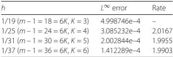
Clearly the errors appear to be of orderO(h2_{) in Table 1.}

Next, we present the error results of Algorithm 1 in terms of the absolute errors and the relative errors, where the absolute error (A. E.) is defined by

en_j =un_j –u(xj,tn),

and the relative error (R. E.) is defined by

En_j = e

n j

|u(xj,tn)|×

100%.

Tables 2 and 3 display the absolute errors and the relative errors obtained by the pre-sented Algorithm 1 forh= 1/19 (i.e.,m–1 = 18 = 6K,K= 3),h= 1/25 (i.e.,m–1 = 24 = 6K,

Table 1 Convergence rate of Algorithm 1 forhatt= 0.4

h L∞error Rate

Table 2 The absolute errors and relative errors of numerical solutions to Example 1 forh= 1/19 (i.e., m– 1 = 18 = 6K,K= 3)

xj Algorithm 1 (t= 0.2) Algorithm 1 (t= 0.4) Algorithm 1 (t= 0.8)

A. E. R. E. A. E. R. E. A. E. R. E.

0.11 0.3731e–3 1.7559e–2 0.5021e–3 1.9312e–2 0.7577e–3 1.9534e–2

0.21 0.6184e–3 1.5420e–2 0.8428e–3 1.7176e–2 1.2739e–3 1.7399e–2

0.31 0.8750e–3 1.5999e–2 1.1881e–3 1.7754e–2 1.7950e–3 1.7976e–2

0.42 0.9753e–3 1.5409e–2 1.3294e–3 1.7165e–2 2.0093e–3 1.7388e–2

0.52 1.0066e–3 1.5469e–2 1.3715e–3 1.7225e–2 2.0729e–3 1.7447e–2

0.63 0.9135e–3 1.5280e–2 1.2463e–3 1.7037e–2 1.8839e–3 1.7259e–2

0.73 0.7582e–3 1.5778e–2 1.0310e–3 1.7534e–2 1.5579e–3 1.7757e–2

0.84 0.5469e–3 1.7563e–2 0.7361e–3 1.9316e–2 1.1109e–3 1.9538e–2

0.95 0.1891e–3 1.7556e–2 0.2545e–3 1.9309e–2 0.3841e–3 1.9532e–2

Table 3 The absolute errors and relative errors of numerical solutions to Example 1 forh= 1/25 (i.e., m– 1 = 24 = 6K,K= 4)

xj Algorithm 1 (t= 0.2) Algorithm 1 (t= 0.4) Algorithm 1 (t= 0.8)

A. E. R. E. A. E. R. E. A. E. R. E.

0.04 0.5579e–4 9.0292e–3 0.7499e–4 9.9277e–3 1.1317e–4 1.0041e–2

0.12 1.6391e–4 9.0313e–3 2.2031e–4 9.9298e–3 3.3247e–4 1.0043e–2

0.24 2.7890e–4 8.2703e–3 3.7803e–4 9.1694e–3 5.7102e–4 0.9283e–2

0.36 3.5674e–4 8.0054e–3 4.8512e–4 8.9048e–3 7.3305e–4 0.9018e–2

0.48 3.8737e–4 7.8818e–3 5.2760e–4 8.7813e–3 7.9739e–4 0.8895e–2

0.60 3.6642e–4 7.8242e–3 4.9945e–4 8.7237e–3 7.5491e–4 0.8837e–2

0.72 2.9685e–4 7.8239e–3 4.0462e–4 8.7235e–3 6.1158e–4 0.8837e–2

0.84 1.8851e–4 7.9457e–3 2.5655e–4 8.8452e–3 3.8769e–4 0.8959e–2

0.96 0.5579e–4 9.0292e–3 0.7499e–4 9.9277e–3 1.1317e–4 1.0041e–2

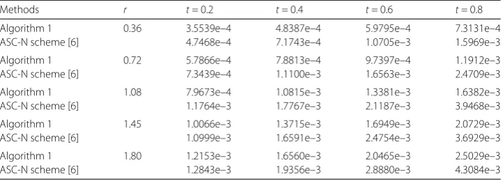
Table 4 Comparisons by the maximum errors to Example 1 forh= 1/19 (i.e.,m– 1 = 18 = 6K,K= 3)

Methods r t= 0.2 t= 0.4 t= 0.6 t= 0.8

Algorithm 1 0.36 3.5539e–4 4.8387e–4 5.9795e–4 7.3131e–4

ASC-N scheme [6] 4.7468e–4 7.1743e–4 1.0705e–3 1.5969e–3

Algorithm 1 0.72 5.7866e–4 7.8813e–4 9.7397e–4 1.1912e–3

ASC-N scheme [6] 7.3439e–4 1.1100e–3 1.6563e–3 2.4709e–3

Algorithm 1 1.08 7.9673e–4 1.0815e–3 1.3381e–3 1.6382e–3

ASC-N scheme [6] 1.1764e–3 1.7767e–3 2.1187e–3 3.9468e–3

Algorithm 1 1.45 1.0066e–3 1.3715e–3 1.6949e–3 2.0729e–3

ASC-N scheme [6] 1.0999e–3 1.6591e–3 2.4754e–3 3.6929e–3

Algorithm 1 1.80 1.2153e–3 1.6560e–3 2.0465e–3 2.5029e–3

ASC-N scheme [6] 1.2843e–3 1.9356e–3 2.8880e–3 4.3084e–3

K= 4) att= 0.2,t= 0.4, andt= 0.8, when takingr= 1.5 (r=τ/h2_{). From Tables 2 and 3, it}

is obvious that our algorithm has high accuracy.

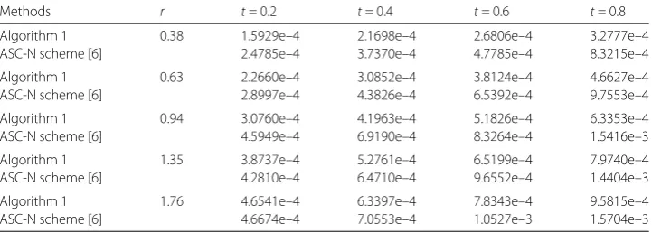
Now, we compare Algorithm 1 with the ASC-N scheme in [6] by the maximum errors for h= 1/19 (i.e.,m– 1 = 18 = 6K,K= 3),h= 1/25 (i.e.,m– 1 = 24 = 6K,K= 4), andh= 1/31 (i.e.,m– 1 = 30 = 6K,K= 5) at different timet= 0.2,t= 0.4,t= 0.6,t= 0.7, andt= 0.8. With the increase in computation time, the errors of the ASC-N scheme in [6] increase more than those of Algorithm 1 for differentr(r=τ/h2) in Tables 4 and 5. We can see that Algorithm 1 has higher accuracy. We consider an example forh= 1/121 (m– 1 = 120 = 6K, K= 20) with large grid ratior= 15 (r=τ/h2_{). Table 6 shows that Algorithm 1 has better}

Table 5 Comparisons by the maximum errors to Example 1 forh= 1/25 (i.e.,m– 1 = 24 = 6K,K= 4)

Methods r t= 0.2 t= 0.4 t= 0.6 t= 0.8

Algorithm 1 0.38 1.5929e–4 2.1698e–4 2.6806e–4 3.2777e–4

ASC-N scheme [6] 2.4785e–4 3.7370e–4 4.7785e–4 8.3215e–4

Algorithm 1 0.63 2.2660e–4 3.0852e–4 3.8124e–4 4.6627e–4

ASC-N scheme [6] 2.8997e–4 4.3826e–4 6.5392e–4 9.7553e–4

Algorithm 1 0.94 3.0760e–4 4.1963e–4 5.1826e–4 6.3353e–4

ASC-N scheme [6] 4.5949e–4 6.9190e–4 8.3264e–4 1.5416e–3

Algorithm 1 1.35 3.8737e–4 5.2761e–4 6.5199e–4 7.9740e–4

ASC-N scheme [6] 4.2810e–4 6.4710e–4 9.6552e–4 1.4404e–3

Algorithm 1 1.76 4.6541e–4 6.3397e–4 7.8343e–4 9.5815e–4

ASC-N scheme [6] 4.6674e–4 7.0553e–4 1.0527e–3 1.5704e–3

Table 6 Maximum error comparison forr= 15,h= 1/121 (m– 1 = 120 = 6K,K= 20)

Algorithm 1 ASC-N method [6] AGE method [3]

t= 0.2 1.3994e–4 1.4759e–4 1.2717e–3

t= 0.4 3.2238e–4 2.8034e–4 3.2242e–3

t= 0.6 5.0639e–4 6.5004e–4 6.2125e–3

t= 0.8 6.9237e–4 8.3824e–4 9.2284e–3

Example2

⎧ ⎪ ⎪ ⎪ ⎪ ⎪ ⎨ ⎪ ⎪ ⎪ ⎪ ⎪ ⎩

∂u

∂t –

∂2u

∂x2 – ∂2u

∂y2 =f(x,y,t), (x,y)∈,t∈(0, 1], u(x,y, 0) =sin(πx)sin(πy), (x,y)∈, u(0,y,t) =u(1,y,t) = 0, y∈[0, 1],t∈(0, 1], u(x, 0,t) =u(x, 1,t) = 0, x∈[0, 1],t∈(0, 1],

(36)

where the domain is= (0, 1)×(0, 1) and the right-hand side function is

f(x,y,t) =1 + 2π2etsin(πx)sin(πy). (37)

The corresponding exact solution is

u(x,y,t) =etsin(πx)sin(πy). (38)

Table 7 The maximum errors of Algorithm 2 to Example 2 forτ= 0.0004

h= 1/19 h= 1/25 h= 1/31 h= 1/37

t= 0.2 6.0275e–4 1.5451e–4 8.0677e–5 4.9096e–5

t= 0.4 4.4976e–4 1.9272e–4 1.0052e–4 6.1127e–5

t= 0.5 5.1593e–4 2.1305e–4 1.1113e–4 6.7574e–5

t= 0.6 5.7284e–4 2.3546e–4 1.2282e–4 7.4684e–5

t= 0.8 7.0014e–4 2.8760e–4 1.5001e–4 9.1219e–5

Table 8 Comparison of three schemes calculation time forr= 1.2 att= 0.5

h Algorithm 2 C-N scheme ASC-N scheme

1/37 (m– 1 = 36 = 6K,K= 6) 16.4121 s 20.2625 s 16.7089 s 1/49 (m– 1 = 48 = 6K,K= 8) 41.4226 s 49.9863 s 41.0513 s 1/61 (m– 1 = 60 = 6K,K= 10) 148.2623 s 175.2632 s 146.0665 s 1/91 (m– 1 = 90 = 6K,K= 15) 981.5628 s 1167.2047 s 966.9273 s

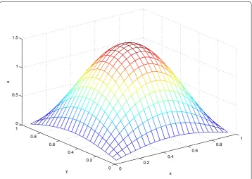
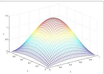
Figure 1The exact solutions att= 0.4

Based on the experiments above, Algorithm 1 and Algorithm 2 presented in this paper are suitable and efficient for solving parabolic equations.

8 Conclusion

high-Figure 2The numerical solutions forr= 1.0,h= 1/19 att= 0.4

Figure 3The numerical solutions forr= 1.0,h= 1/25 att= 0.4

Figure 4The numerical solutions forr= 1.0,h= 1/37 att= 0.4

Acknowledgements

The authors would like to thank the anonymous referees for helpful comments and suggestions. This research is supported by the National Natural Science Foundation of China (91130022, 10971159) and the Doctoral Fund of Ministry of Education of China (20130141110026).

Competing interests

The authors declare that they have no competing interests.

Authors’ contributions

All authors contributed equally and significantly in writing this article. All authors read and approved the final manuscript.

Publisher’s Note

Springer Nature remains neutral with regard to jurisdictional claims in published maps and institutional affiliations.

Received: 14 January 2018 Accepted: 25 April 2018 References

1. Evans, D.J., Abdullah, A.R.B.: Group explicit method for parabolic equations. Int. J. Comput. Math.14, 73–105 (1983) 2. Saul’yev, V.K.: Integration of Equations of Parabolic Type by Method of Nets, New York (1964)

3. Evans, D.J.: Alternating group explicit method for the diffusion equation. Appl. Math. Model.9, 201–206 (1985) 4. Zhang, B.: Alternating segment explicit–implicit method for the diffusion equation. Chin. J. Numer. Methods Comput.

Appl.41, 245–251 (1991)

5. Chen, J., Zhang, B.: A class of alternating block Crank–Nicolson method. Int. J. Comput. Math.45, 89–112 (1991) 6. Zhang, B., Li, W.: On alternating segment Crank–Nicolson scheme. Parallel Comput.20, 897–902 (1994) 7. Cao, J.Y., Zhang, D.K.: A new parallel algorithm for the parabolic equation. Guizhou Sci.25(2), 27–33 (2007) 8. Evans, D.J., Abdullah, A.R.B.: A new explicit method for the diffusion–convection equation. Comput. Math. Appl.11,

145–154 (1985)

9. Lu, J., Zhang, B., Xu, T.: Alternating segment explicit–implicit method for the convection–diffusion equation. Chin. J. Numer. Methods Comput. Appl.3, 161–167 (1998)

10. Wang, W.: A class of alternating segment Crank–Nicolson methods for solving convection–diffusion equations. Computing73, 41–55 (2004)

11. Zhu, S., Yuan, G., Shen, L.: Alternating group explicit method for the dispersive equation. Int. J. Comput. Math.75, 97–105 (2000)

12. Zhu, S., Zhao, J.: The alternating segment explicit–implicit scheme for the dispersive equation. Appl. Math. Lett.14, 657–662 (2001)

13. Wang, W., Fu, S.: An unconditionally stable alternating segment difference scheme of eight points for the dispersive equation. Int. J. Numer. Methods Eng.67, 435–447 (2006)

15. Wang, W.Q., Zhang, Q.: A highly accurate alternating 6-point group method for the dispersive equation. Int. J. Comput. Math.87(7), 1512–1521 (2010)

16. Guo, G., Lü, S., Liu, B.: Unconditional stability of alternating difference schemes with variable time step lengths for dispersive equation. Appl. Math. Comput.262, 249–259 (2015)

17. Guo, G., Liu, B.: Unconditional stability of alternating difference schemes with intrinsic parallelism for the fourth-order parabolic equation. Appl. Math. Comput.219, 7319–7328 (2013)

18. Guo, G., Zhai, Y., Liu, B.: The alternating segment explicit–implicit scheme for the fourth-order parabolic equation. J. Inf. Comput. Sci.10, 2981–2991 (2013)

19. Guo, G., Lü, S.: Unconditional stability of alternating difference schemes with intrinsic parallelism for two-dimensional fourth-order diffusion equation. Comput. Math. Appl.71, 1944–1959 (2016)

20. Du, Q., Mu, M., Wu, Z.: Efficient parallel algorithms for parabolic problems. SIAM J. Numer. Anal.39(5), 1469–1487 (2001)

21. Zhuang, Y., Sun, X.: Stabilized explicit–implicit domain decomposition methods for the numerical solution of parabolic equations. SIAM J. Sci. Comput.24, 335–358 (2002)

22. Shi, H., Liao, H.: Unconditional stability of corrected explicit–implicit domain decomposition algorithms for parallel approximation of heat equations. SIAM J. Numer. Anal.44, 1584–1611 (2006)

23. Boglaev, I.: Domain decomposition for a parabolic convection–diffusion problem. Numer. Methods Partial Differ. Equ. 22, 1361–1378 (2006)

24. Dryja, M., Tu, X.: A domain decomposition discretization of parabolic problems. Numer. Math.107, 625–640 (2007) 25. Li, C., Yuan, Y.: A modified upwind difference domain decomposition method for convection–diffusion equations.

Appl. Numer. Math.59, 1584–1598 (2009)

26. Liang, D., Du, C.: The efficient S-DDM scheme and its analysis for solving parabolic equations. J. Comput. Phys.272, 46–69 (2014)

27. Arrarás, A., Gaspar, F.J., Portero, L., Rodrigo, C.: Domain decomposition multigrid methods for nonlinear reaction–diffusion problems. Commun. Nonlinear Sci. Numer. Simul.20, 699–710 (2015)

28. Kumar, S., Kumar, M.: An analysis of overlapping domain decomposition methods for singularly perturbed reaction–diffusion problems. J. Comput. Appl. Math.281, 250–262 (2015)

29. Zhou, Z., Liang, D.: A time second-order mass-conserved implicit–explicit domain decomposition scheme for solving the diffusion equations. Adv. Appl. Math. Mech.9(4), 795–817 (2017)

30. Zhou, Y.: Finite difference method with intrinsic parallelism for quasilinear parabolic systems. Beijing Math.2, 1–19 (1996)

31. Zhou, Y.: General finite difference schemes with intrinsic parallelism for nonlinear parabolic system. Beijing Math.2, 20–36 (1996)

32. Zhou, Y., Shen, L., Yuan, G.: Some practical difference schemes with intrinsic parallelism for nonlinear parabolic systems. Chin. J. Numer. Methods Comput. Appl.19, 46–57 (1997)

33. Yuan, G., Shen, L., Zhou, Y.: Unconditional stability of alternating difference schemes with intrinsic parallelism for two-dimensional parabolic systems. Numer. Methods Partial Differ. Equ.15, 625–636 (1999)

34. Sheng, Z., Yuan, G., Hang, X.: Unconditional stability of parallel difference schemes with second order accuracy for parabolic equation. Appl. Math. Comput.184(2), 1015–1031 (2007)

35. Yuan, G., Sheng, Z., Hang, X.: The unconditional stability of parallel difference schemes with scheme order convergence for nonlinear parabolic system. Numer. Methods Partial Differ. Equ.20(1), 45–64 (2007)

36. Zhuang, Y.: An alternating explicit–implicit domain decomposition method for the parallel solution of parabolic equations. J. Comput. Appl. Math.206, 549–566 (2007)

37. Kellogg, R.B.: An alternating direction method for operator equations. J. Soc. Ind. Appl. Math.12, 848–854 (1964) 38. Zeng, F., Zhang, Z., Karniadakis, G.E.: Fast difference schemes for solving high-dimensional time-fractional