R E S E A R C H
Open Access
Optimal power allocation on discrete energy
harvesting model
Xiaolei Wang
1†, Jie Gong
1*†, Congshi Hu
2†, Sheng Zhou
1†and Zhisheng Niu
1†Abstract
This paper studies the power allocation problem in energy harvesting systems with finite battery. We adopt the discretized energy arrival and power allocation model. Hence, the service process can be modeled as a finite state Markov chain. Based on the discretized model, we analyze the stationary distribution of the Markov chain and formulate the utility maximization problem, which is then reformed as a linear programming problem. By analyzing the linear programming problem, we provide some intuition on the structure of the optimal power allocation policy and find the condition in which the greedy power allocation is optimal. Numerical simulations show the influence of the energy arrival process on the optimal power allocation policy, and the results are consistent with our analysis.
Keywords: Energy harvesting; Markov chain; Power allocation
1 Introduction
With increasing CO2 emissions in communication net-works, how to realize green communications in the future has become an important and hot topic in the academic society. Besides the energy-efficient protocol design to reduce the energy consumption of the conventional wire-less systems, utilizing renewable energy (e.g., solar or wind energy) to power on communication devices, namely, the energy harvesting technology, provides a new way for green by exploiting sustainable energy sources and hence is a promising solution to achieve environment-friendly communications. Recent developments in hard-ware have made the energy harvesting technology feasible for modern communication systems. For instance, a wind-powered tower for wireless base stations has been designed by Ericsson [1]. However, due to the randomness of the energy arrival process, how to optimally allocate the harvested energy is a challenging issue.
In recent years, a lot of research efforts have been focused on the energy harvesting systems. For the addi-tive white Gaussian noise (AWGN) channel, the problem of minimizing the transmission completion time with
*Correspondence: [email protected] †Equal contributors
1Tsinghua National Laboratory for Information Science and Technology, Department of Electronic Engineering, Tsinghua University, 100084 Beijing, People’s Republic of China
Full list of author information is available at the end of the article
infinite battery capacity in non-fading channel is stud-ied in [2] for two scenarios, i.e., all packets are ready before transmission and packets arrive during transmis-sion. Tutuncuoglu [3] finds the optimal transmission policy to maximize the short-term throughput with lim-ited energy storage capacity, and exploits the relation between the throughput maximization and the trans-mission completion time minimization. For the fading channel, authors in [4] propose the directional water-filling (WF) algorithm which is proved throughput opti-mal for greedy source. Similar result is obtained in [5], which further considers the optimal solution with causal information. The algorithm is then extended to multi-ple antennas scenario in [6], where the spatial-temporal WF is proposed. Further, considering the dynamic data arrival with hybrid energy harvesting and power grid supplies, [7] proposes the optimal reverse multi-stage WF policy. Considering the circuit power consumption, a two-phase transmission policy is shown to be opti-mal [8]. In [9], the authors study the throughput maxi-mization problem for the orthogonal relay channel with energy harvesting source and relay nodes under the deterministic model and show the structure of the opti-mal source and relay power allocation. Although the above algorithms give some insights about the optimal solution, they assume that all the energy arrival, the channel fading, and the data arrival must be explicitly known before transmission, which is called the offline
condition. Since the solutions based on the offline con-dition require accurate predictions for the system states, they are not always applicable in real communication systems.
Based on the online condition that only the past and current system states can be known, researchers have studied the optimal and sub-optimal power allocation policies in some special scenarios. Sharma [10] identi-fies throughput optimal and mean delay optimal energy management policies and shows a greedy policy to be optimal in low SNR regime with infinite battery capacity. And a throughput maximization algorithm in point-to-point communications with causal information based on Markov decision process (MDP) [11] approach is pro-posed in [12]. Recent work [13] studies the finite-horizon scheduling problem with discrete rates and proposes a low complexity threshold-based policy. However, the proper-ties of the optimal solution can not be directly obtained via MDP approach. In addition, the MDP approach expe-riences very high computational complexity due to the curse of dimensionality, hence may not be applicable when the system state space grows large. From the informa-tion theory perspective, [14] studies the channel capacity of energy harvesting links with finite battery capacity and proves that the Markovian energy management poli-cies are sufficient to achieve the capacity. Besides the throughput maximization problems, some other issues on the energy harvesting systems, such as the quality of service (QoS), the energy efficiency, and etc. are also studied. Huang [15] studies the utility optimization prob-lem in energy harvesting networks under limited average network congestion constraint and develops a close-to-optimal algorithm using the Lyapunov optimization the-ory, which jointly manages the power allocation and the data access control. As the renewable energy is usually dis-tributed asymmetrically in space domain, there are some papers considering the energy cooperation problem to balance the harvested energy in different places, including cellular network planning [16] and power grid energy sav-ing [17], so that the overall system energy efficiency can be improved. But still, under the dynamic property of the energy harvesting process, how to allocate the energy to achieve the optimal system performance in general case is still an open question. It is desirable to explore the closed-form analytical solution for the online condition with some statistic characteristic of the energy harvesting process.
In this paper, we consider the power allocation problem in energy harvesting capacity to achieve the optimal sys-tem utility. Specifically, we study a single link with renew-able energy transmitter, which only has the casual state information, including the distribution of the energy har-vesting process, the past, and the current battery energy state. We model the energy arrival, storage, and usage
as a discrete model and derive the optimal solution with closed-form expressions. The main contributions of this paper are presented as follows.
• We propose the discrete model for the energy harvesting system analysis. On one hand, the digital equipment has been widely used in modern communication systems, and it is feasible to give a discrete model for the energy harvesting process. On the other hand, the discrete model enable us to give a Markovian analysis and get some interesting
closed-form analytical solution.
• For the independent identically distributed (i.i.d.) energy arrival process, we show the optimal solution can be obtained by solving a linear programming problem. Based on the linear programming formulation, we get some properties of the optimal power allocation policy and find the condition under which the greedy policy is optimal.
• Through extensive numerical simulations, we discuss the influence of the statistics of the energy arrival process on the optimal power allocation policy, which is shown consistent with our mathematical analysis.
The rest of the paper is organized as follows. Section 2 presents the system model. The problem is formulated and analyzed in Sections 3 and 4, respectively. Some numerical results are provided in Section 5 to evaluate the performance analysis. Finally, Section 6 concludes the paper.
Notations:Bold upper case and lower case letters denote matrices and vectors, respectively.(·)Tdenotes the trans-pose of a matrix or a vector.0n×mand1n×mrepresent the n×mmatrices with all elements equal to 0 and 1, respec-tively. Ifn=m, they can be simplified as0nand1n.Inis
then×nunit matrix.Eis the expectation operation.
2 System model
We consider a single link time-slotted wireless commu-nication system with slot length Tf. The transmitter is
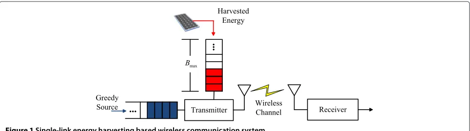
powered by renewable energy, which is harvested from the environment and stored in a battery with finite capac-ityBmax. The greedy data source is assumed to focus on the utility maximization with efficient harvested energy usage. The system model is illustrated in Figure 1. The utility is assumed to be a strictly concave and increas-ing function of allocated transmit power. As the slot length is fixed, the utility can be equivalently viewed as a function of used energySt, denoted byu(St). While the
transmit energyStdepends on the system state, i.e., the
amount of energy stored in the battery in slott, denoted byEt.
B
Figure 1Single-link energy harvesting based wireless communication system.
allocation policy determines the amount of used energy
St based on the system state Et (red bar in the figure). Considering the energy causality constraint, the allocated energy cannot exceed the energy stored, i.e., St ≤ Et.
DenoteE˜t as the transition state after the power
alloca-tion process and before the energy harvesting process. According to the power allocation result, the transitional system state updates asE˜t = Et−St. Then, the amount
of energyAtis harvested during slottis stored into the
battery at the end of the slot. Note that the battery energy cannot exceed the battery capacity. Hence, the additional energy will be wasted if the battery is full. As a result, the system state is updated according to the following equation:
Et+1=min{Et−St+At,Emax}. (1)
In this paper, we consider a discrete system model, i.e., the energy is discretized with unit E. In the dis-crete model, the battery capacity can be expressed as
Bmax = NE, whereNis an integer. Hence, for the ease of description, we omitE and denote the system state asEt = n,n = {0, 1,. . .,N} which indicates thatnE
amount of energy is stored in the battery. Besides, the energy arrivalAtand the power allocationStare also
dis-cretized with the unit energyE, which will be detailed in the following subsections.
2.1 Energy arrival model
The amount of energy arrived in each time slot is assumed to be i.i.d. and takes non-negative integer values. The distribution of the energy arrival is expressed as:
Pr [At=k]=hk, k=0, 1, 2,. . ., (2)
wherehk ≥0,
khk =1.
After harvesting the arrived energy, the system state transits from the transition stateE˜tto the state of the next
slotEt+1. The state transition probability matrix due to energy arrival and harvesting process can be expressed as an(N+1)×(N+1)matrixH, namely,harvesting matrix, with elementsHi,jdenoting the transition probability from
˜
Et = i to Et+1 = j by harvesting (j − i)E amount of energy. As the amount of harvested energy is non-negative,His an upper triangular matrix. The elements of Hcan be calculated as:
Hi,j=
⎧ ⎪ ⎪ ⎪ ⎪ ⎨ ⎪ ⎪ ⎪ ⎪ ⎩
0, i>j,
hj−i, i≤j<N,
1−N−i−1
k=0
hk, i<j=N,
1, i=j=N.
(3)
Note thatj=Nrepresents that the battery is full. In this case, the amount of arrived energy larger thanN−iwill tend to the same stateEt+1 = N. Hence, the probability
Figure 2Discrete system state transition model.At the beginning of slott,Stis used to transmit. At the end of the slot,Atis arrived and stored
forj = N is a summation of energy arrival distribution that satisfyAt≥N−i.
2.2 Power allocation policies
Recall that the power allocation policies only depend on the current system state. Similar as the energy arrival model, we express the state transition probability matrix between Et and E˜t as a policy matrix P with elements pi,j ∈ {0, 1},∀i,jdenoting the event of using(i−j)unites
of energy in state Et = i. Then, the allocated power is
calculated as (i − j)E/Tf. Since the allocated energy
is non-negative, all the non-zero elements of the policy matrixPis on the left side of the diagonal elements, i.e.:
pi,j=0, ∀i<j, (4)
Besides, the deterministic policy tells us that only one action will be taken in each state. Hence, there is and only is one non-zero element in each row, which is as follows:
i
j=0pi,j=1, ∀i. (5)
Note thatpi,jis relaxed to take the value between 0 and
1 for the ease of mathematical formulation and theoreti-cal analysis in the next section. However, a deterministic optimal policy is ultimately obtained through our solu-tion, which means that the relaxed problem is equivalent with the original problem. We will discuss this issue in detail later.
2.3 Utility model
For any amount of allocated energy St, there is a
cor-responding utility u(St). Since we consider the discrete
energy model, the utility also takes value from a finite set{u0,u1,. . .,uN}. Specifically,uk is the utility when the
amount of kE energy is allocated in a slot, i.e., uk = u(kE). As mentioned before, it is assumed to be increas-ing and strictly concave for k ≥ 0 and u0 = 0. For instance, if the optimal channel coding scheme with ran-domly generated codes is adopted, we can achieve the channel capacity given by:
uk=
1 2log2
1+ kE
Tfσ2
, (6)
whereσ2is the noise power. It is the well-known Shan-non’s equation [18]. Also, some other utility functions can be used, as long as they satisfy the monotonicity and the concavity properties.
3 Problem formulation
In this section, we formulate the utility maximization problem and transform the problem formulation into
lin-ear programming based on the Markovian property. We also simply discuss the linear programming problem for-mulation from the MDP point of view.
3.1 Utility maximization and Markov chain-based formulation
The objective of our problem is to maximize the average utility over a long time period, i.e.:
max lim
T→+∞E
1
T T
t=1
u(St)E1=k0
, (7)
where k0 is the initial battery energy, and the allocated energy St is determined by the battery energy state Et.
Notice that we can apply MDP approach [11] to solve the infinite horizon average utility maximization with finite number of states (the number of system states, i.e., the battery energy states isN). However, the MDP approach usually encounters the curse of dimensionality problem. In addition, the structure of the optimal policy is not clear as the MDP only outputs numerical results. To avoid the drawbacks of the MDP approach and analyze the opti-mal power allocation policy in detail, we consider to deal with the problem using linear programming. Specifically, for a given power allocation policy, the battery energy state forms a Markov chain. Firstly, we have the following lemma.
Lemma 1. The problem (7) is irrelevant with the initial state k0.
Proof. The Markov chain with battery energy as state satisfies the weak accessibility ([11], Def. 4.2.2), as for a given energy arrival distribution {h0,h1,. . .} and for any states i,j, we can always find a stationary policy so that stateiis accessible from statej. According to ([11], Prop. 4.2.3), the optimal average utility is the same for all initial states.
Actually, the conclusion of Lemma 1 is easy to be under-stood as we consider the long-term average performance; the influence of the state at some specific time is negligi-ble. Based on Lemma 1, we only need to consider the sta-tionary behavior of the Markov chain. For a given power allocation policyP, there always exists a stationary sys-tem state distributionπ = [π0,π1,. . .,πN]T,Ni=0πi =
1,πi≥0,∀ithat satisfies:
πTPH=πT, (8)
to stateEt+1. With the stationary distribution, the original problem (7) can be reformulated as:
P-1: max
where the harvesting matrix H and the utility function
uk,k = 0,. . .,N are predefined and (9b) is the
expan-sion of (8). Note that different power allocation policies lead to different stationary distributions. On the contrary, if the state distribution varies, the optimal power alloca-tion policy also changes. Hence, the unknown variables include both the power allocation policypi,j,i≥j
and the stationary distribution{πi}, which need to be jointly
considered and optimized. Aspi,j ∈ {0, 1}, it is a mixed
optimization problem combining both integer program-ming and linear programprogram-ming, which is difficult to be solved. To make it tractable, we transform the problem into a linear programming optimization problem in the rest of this section.
3.2 Problem reformulation with linear programming Firstly, we relax the constraint (9e) and reformulate the problem as:
wherepi,jbecomes continuous variable, which can be
con-sidered as a probabilistic power allocation policy. In the next section, we will prove that the relaxation does not change the optimal solution. In other words, the optimal policy p∗i,j obtained by solving P-1R turns out to be of integer value.
Obviously, the problem P-1Ris not a convex optimiza-tion problem since there is productπipi,jin the constraint
(9b). To solve this problem, we transform it by multiplying πion both sides of the constraints (9c):
i
the stationary stateidoes not exist, leading to no influence on the total utility. Hence, by denotingfi,j=πipi,j, we can
get the equivalent optimization problem of P-1as:
P-2: max
We can see that the optimization problem P-2is a linear optimization as the objective function and the constraints are all linear functions. By solving the optimalfi,jandπi, since the system stateihas no influence on the total utility. Actually,fi,jis the probability that the system state isiand j−iunits of energy is used.
In the objective function of problem P-2, the variable πiis not presented. And iffi,j is known,πican be
calcu-lated via (12b) or (12c). Substitutingπibyik=0fi,kin P-2,
the optimalfi,j
Note that the right-side inequality of (12e) and the con-straint (12f) is omitted in P-3as they are guaranteed by (14c) and (14d). Further, the problem P-3can be expressed in a matrix form as:
P-3M: max uTf (15a)
The problem can be further simplified based on the following lemma.
Lemma 2. The constraint (15b) can be equivalently writ-ten as:
prove that the sum of each column ofAˆ equals to 1. Con-sequently, we have11×1
2(N+1)(N+2) ˆ
Af =11×1
2(N+1)(N+2)f,
which means that the last constraint in (22) can be obtained by the summation of the first (N + 1) equal-ity constraints, hence naturally holds as long as the other constraints are satisfied. As a result, (19) is obtained by removing the last constraint in (22). As the matrixBis invertible, the constraint (19) is equivalent with (15b).
Based on Lemma 2, the number of the equality con-straints is reduced from (N +2) to (N+ 1). Note that the rank ofAˆ is(N+1)since the first(N+1)columns form an(N+1)unit matrix, which means that the equality constraints are irreducible. We re-write the problem as:
P-4: max uTf (23a)
s.t. Afˆ =h0, (23b)
f≥01
2(N+1)(N+2)×1, (23c)
In the rest of the paper, we focus on the solution for the problem P-4. As long as it is solved, the original problem P-1Ris also solved. Specifically, the stationary distribu-tionπcan be calculated by (12b) or (12c), and the power allocation policy can be obtained by (13). In addition, the optimality proof of deterministic solution given in the next section guarantees the equivalence between prob-lem P-4 and problem P-1. Hence, problem P-1 is also solved.
Remark 3. The optimization problem P-4 can also be derived based on the MDP theory [11]. Specifically, for a given time indext, the system state xt ∈ {0,. . .,N}is
the battery energy state, the actionat(xt) ∈ {0,. . .,xt}is
the allocated energy. For the finite state problems, there exists an optimal stationary policy. Hence, we can omit the time index ofat. Then, the cost functiong(xt,a(xt))= −ua(xt) is the negative utility, and the state transition is calculated aspij(a(i))=Hi−a(i),j. We re-write the average
The optimal policy satisfies the Bellman’s equation ([11], Prop. 4.2.1), which in the problem (24) takes the form:
λ+s(i)= min a(i)∈{0,...,i}
⎡
⎣g(i,a(i))+
N
j=0
pij(a(i))s(j)
⎤
⎦,i=0,. . .,N.
(25)
with a scalarλanda vectors. The optimal costλ∗can be determined by solving the following linear programming problem ([11], Sec. 4.5):
max λ (26a)
s.t. λ +s(i)≤g(i,a(i))+ N
j=0
pij(a(i))s!j",
i =0,. . .,N,a(i)=0,. . .,i. (26b)
Applying the duality theory of linear programming ([19], Chap. 5), we can exactly get the linear program formula-tion as P-3, and hence, P-4is formulated. However, with Markov chain analysis instead of MDP theory, we can get the clear physical meaning of the variablefi,j.
Remark 4. When solving the original problem P-1, it requires an exhaustive search over all the possible values of the parameterspi,j∈ {0, 1},∀i≥j, which is of
exponen-tial complexity. While the complexity of solving the linear programming problem P-4 depends on the numerical algorithms which we apply. The most popular algorithms for solving linear programming problem are thesimplex algorithmand theinterior point algorithm[19]. It has been analyzed that the simplex algorithm is of exponential com-plexity in the worst case [20], while the comcom-plexity of a specific problem is case by case. We will show in the following section that in some cases, the optimal solu-tion can be found without iterasolu-tion. On the other hand, the interior point algorithm is of polynomial complex-ity. In summary, the complexity of the proposed linear programming is lower than that of the exhaustive search algorithm.
4 Optimal solution analysis
It is difficult to give an analytical solution for general con-ditions ofHandu. In this section, we try to find some properties on the structure of the optimal power alloca-tion policy and derive the condialloca-tion in which some simple policy is optimal. We firstly present some general results about the optimal policy.
4.1 General properties
With a quick observation, we can firstly get the following property.
Proposition 1. (Feasibility)The optimal solutionf∗for the problem P-4exists.
Proof.Firstly, the problem P-4 is feasible as we can at least find one solution satisfying all the constraints. For instance:
fg=
hT0, 0,. . ., 0 T
, (27)
is feasible for the problem.
Secondly, the feasible region for the linear programming problem is finite according to the constraintsf ≥ 0and 11×1
2(N+1)(N+2)·f=1. Hence, the optimal solution exists.
Proposition 1 tells us that the problem is feasible, and the existence of the optimal solution is guaranteed by the finite state constraint.
Lemma 3. The optimal solutionf∗for the problem P-4can be achieved by the vector with at most(N+1)non-zero elements.
Proof.The optimal solution for a linear programming can be achieved by itsbasic feasible solution[19], of which the number of non-zero elements is no more than the rank of Aˆ. Since the rank of Aˆ is(N + 1), its basic feasible solution has at most(N+1)non-zero elements.
The geographic explanation of Lemma 3 is that for a linear programming problem, the optimal solution can always be found at the vertex (corresponding to the basic feasible solution) of the convex polyhedron defined by the constraints (23b) and (23c) [19]. In this sense, we only need to focus on the basic feasible solutions with relatively small number of non-zero elements. However, it is not guaranteed that the optimal solution must have no more than(N+1)non-zero elements. For instance, if there are two vertexes to be optimal, all the linear combinations of the two vertexes are also optimal.
Based on Lemma 3, we can guarantee the deterministic optimal policy can be obtained.
Proposition 2. (Deterministic optimal solution) The optimal solution of P-4can be achieved by a deterministic power allocation policy, i.e., p∗i,j∈ {0, 1}.
If for some k,πk∗ = 0, the statek is a transient state. We can erase all the elements related withπk∗in the prob-lem formulation without changing the optimal solution. Specifically, in the original problem, by removing thek -th row andk-th column of the matrixPHin (8), thek-th constraint in (9b), and the elements related withπkin (9a)
and (9d), the optimal solution is not changed. Through the same deduction of the previous section, we can con-clude the similar lemma that the optimal solution can be achieved with at most N non-zero elements. Simi-larly, we can provep∗i,j ∈ {0, 1},∀i = k. Then, by setting
p∗i,0 = 1, a deterministic optimal policy is also obtained. The proof can also be extended to the case that for several
ks,πk∗=0.
Proposition 2 guarantees that a deterministic optimal power allocation policy can always be found. In fact, the deterministic optimal policy corresponds to the optimal basic feasible solution. Hence, in the sense of determin-istic policy, the equivalence between P-4and P-1, or in other words, the equivalence between P-1R and P-1 is guaranteed. By finding the optimal basic feasible solution of P-4, we can obtain the deterministic optimal power allocation policy for the original problem P-1. Again as discussed in the paragraph below Lemma 3, if there are two basic feasible solutions achieving optimal, the lin-ear combination of the two solutions correspond to the probabilistic optimal policy. In practice, the deterministic optimal policy is desirable and also sufficient.
Theorem 1. (Structure of optimal policy)For the opti-mal power allocation policyP∗, if p∗i,j>0andπi∗>0, for any m that satisfiesπm∗ >0and m>i, we have:
p∗m,n=0,∀n<j. (28)
Proof. See Appendix 1.
Theorem 1 demonstrates that for the optimal policy, if k units of energy is allocated in statei, the allocated amount of energykin the next statei+1 will not increase drastically, i.e.,k−k≤1. The theorem can also be equiv-alently described asp∗m,n = 0,∀n > j, where πm∗ > 0 andm < i. Notice that the conditionπi∗ > 0 indicates that statei is not a transient state. For a transient state, any power allocation policy is applicable as it does not change the objective. Hence, the conclusion does not hold for transient states.
4.2 Optimality of greedy policy
According to the feasible solution example (27), we can get that pi,0 = 1,∀i, which turns out to be the greedy
policy, i.e., in each slot, all the available energy in the bat-tery is used up. In general, the greedy policy is not optimal.
However, the following theorem provides the condition on which it is optimal.
Theorem 2. (Greedy optimal policy)If
N−1
i=0
hi(ui−ui+1)+uN −uN−1≥0, (29)
the optimal solution for P-4isf∗=fg. The optimal power allocation is the greedy algorithm, which means that we use up all the available energy in every slot. The stationary distribution of the system state isπ=h0.
Proof. See Appendix 2.
For the ease of understanding the greedy optimal condi-tion, we rewrite (29) as:
N−1
i=0
hiui≤1, (30)
where
ui=
ui+1−ui uN−uN−1
,i=0,. . .,N−1 (31)
is the relative utility gain by increasing one unit energy in power allocation statei. Thus, given the utility function, the condition can be viewed as the case that the weighted sum of energy arrival distribution up toN−1 weighted by relative utility gain is no more than 1. Sinceui≥1 and is
decreasing function ofi, the condition holds when the tail probability of energy arrival 1−N−i=01hiis large enough,
and the value ofhiis relatively small wheniis small.
Intu-itively, such kind of energy arrival distribution shows the property that the amount of energy arrival is quite large relative to the battery capacity. Hence, the optimal policy tends to use up all the available energy in the battery in every time slot (i.e., greedy policy). In this case, the battery can store as many energy as it can, and hence, the energy wasted due to the battery overflow is reduced.
On the other hand, with a fixed energy arrival distribu-tion{hi}, we can find the influence of the utility function on the optimality of greedy policy. Specifically, we adopt the Shannon’s capacity as the utility function as expressed in (6). At low signal-to-noise ratio (SNR) regime, i.e., TkE
fσ2 is very small, we have the following approximation:
ui≈ iE
2Tfσ2, (32)
which results inui≈1,∀i. Since{hi}is a probability
capacity gain is linearly proportional to the power alloca-tion. Consequently, the greedy policy is optimal as it not only can obtain the same capacity with the same available energy, but also reduces the amount of wasted energy due to battery overflow.
A quick conclusion based on the Theorem 2 can be obtained as follows:
Corollary 1. If the energy arrival is uniformly distributed between 0 and2h with average arrival rate¯ h, the greedy¯ policy is optimal when:
¯
h≥ uN −u0
2(uN−uN−1)
. (33)
Proof.The energy arrival probability of uniform distri-bution is expressed as:
hi=
1
2h¯,i=0,. . ., 2h¯. (34)
By substitutinghi in (29) with (34) and some derivation,
we can get the condition on the average arrival rate.
5 Numerical results
We calculate some numerical examples of the optimal power allocation to demonstrate the structure and the properties of the optimal policies. We define:
γ = E Tfσ2
(35)
as the reference SNR with one unit of energy, and adopt the Shannon’s equation to calculate the utility, i.e.:
uk=
1
2log2(1+kγ ). (36)
Set N = 10 and γ = 1 as an example, we examine the influence of the random energy arrival process on the optimal power allocation. Specifically, we consider some widely used distributions, including discrete uniform dis-tribution, geometric disdis-tribution, Poisson disdis-tribution, and binomial distribution. DenoteUnif(h¯) as the uniform distribution that takes values in{0, 1,. . ., 2h¯} with mean
¯
h. DenotePoiss(h¯) as the Poisson distribution with mean
¯
h. Denote Geom(p) as the geometric distribution with parameterp; thus, we have:
hi=(1−p)ip,i≥0 (37)
with meanh¯=(1−p)/p. And denoteBin(n,p) as the bino-mial distribution with parameters n,p. The probability density function is as follows:
hi= n!
i!(n−i)!p
i(1−p)n−i, 0≤i≤n, (38)
and the mean value ish¯ = np. Since 0< p< 1, we have
n>h¯. Notice that except for binomial distribution, all the studied distributions have only one parameter.
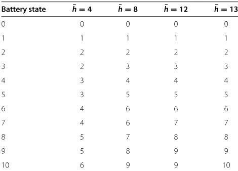
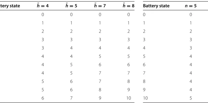
Tables 1, 2, and 3 provides the optimal power allocation policies for uniform distribution, Poisson distribution, and geometric distribution with different mean values. It can be seen that the minimum average arrival rates with which the greedy policy is optimal are different for dif-ferent distributions (h¯ = 13 for uniform distribution,
¯
h = 8 for Poisson distribution, h¯ = 23 for geometric distribution). The result is consistent with our observa-tion. Specifically, ifhi is an increasing function ofi, it is
easier for the greedy policy to be optimal than the case that hi is decreasing. As Poisson distribution increases
before the average value, while geometric distribution is strictly decreasing, consequently higher average energy arrival rate is needed so that greedy policy is optimal for geometric distribution.
Another observation from these results is that differ-ent from infinite battery capacity case where the optimal power will not exceed the average energy arrival rate [[10] Theorem 1], the optimal power exceeds the average energy arrival rate at some cases. As the battery capac-ity is finite, the harvested energy may be wasted when the battery is full. Hence, more energy will be used when the battery energy is close to its limit in order to reduce the wastage of energy.
As the binomial distribution has two parameters, we provide the detailed numerical results in Tables 4, 5, and 6. It can be seen that when the average arrival rateh¯≤7, the greedy policy will never be optimal. While forh¯ = 8, the greedy policy is shown optimal whenn≥11. In addition, whenh¯ ≥ 9, the greedy policy is always optimal for any feasible values ofn>h¯. Since in the binomial distribution,
hi also follows the same feature of Poisson distribution that it firstly increases and then decreases, the threshold ofh¯for the greedy policy to be optimal is relatively low.
Table 1 Optimal power allocation policy for uniform distribution with parameterγ =1
Battery state h¯=4 h¯=8 h¯=12 h¯=13
0 0 0 0 0
1 1 1 1 1
2 2 2 2 2
3 2 3 3 3
4 3 4 4 4
5 3 5 5 5
6 4 6 6 6
7 4 6 7 7
8 5 7 8 8
9 5 8 9 9
10 6 9 9 10
Table 2 Optimal power allocation policy for Poisson distribution with parameterγ =1
Battery state h¯=4 h¯=5 h¯=7 h¯=8
0 0 0 0 0
1 1 1 1 1
2 2 2 2 2
3 3 3 3 3
4 3 4 4 4
5 4 4 5 5
6 4 5 6 6
7 4 5 7 7
8 5 6 7 8
9 5 6 8 9
10 6 7 9 10
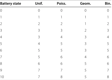
Finally, Tables 7 and 8 compare the optimal policies for the considered distributions at high and low SNR regimes, respectively. It can be seen that at low SNR regime, the optimal policy for any distribution turns out to be the greedy policy. On the other hand, when the SNR is high, it is not true. Besides, the policies for Poisson distribution and binomial distribution are closer to the greedy policy at high SNR regime, which is consistent with the previous analysis.
Another interesting property can be seen from all the results, i.e., the optimal power allocation policy is a non-decreasing function of the battery energy state. Besides, the increasing step is no more than 1, which coin-cides to Theorem 1. The non-decreasing property can be explained as follows. The more the available energy is, the more allocated power is used in order to not only achieve higher data rate but also reduce the energy wastage due to battery overflow. As the battery capacity tends to
Table 3 Optimal power allocation policy for geometric distribution with parameterγ =1
Battery state h¯=4 h¯=13 h¯=22 h¯=23
0 0 0 0 0
1 1 1 1 1
2 2 2 2 2
3 2 3 3 3
4 2 4 4 4
5 3 5 5 5
6 3 5 6 6
7 3 6 7 7
8 4 7 8 8
9 4 8 9 9
10 5 8 9 10
Table 4 Optimal power allocation policy for binomial distribution with parametersγ =1,h¯ =4
Battery state n=5 n=6 n=8 n= +∞
0 0 0 0 0
1 1 1 1 1
2 2 2 2 2
3 3 3 3 3
4 3 3 3 3
5 4 4 4 4
6 4 4 4 4
7 4 4 4 4
8 4 4 5 5
9 4 5 5 5
10 5 5 6 6
infinity, the non-decreasing property still holds as shown in [10].
We also run some simulations to evaluate the perfor-mance of the optimal power allocation policy. For compar-ison, we consider the following two policies as baselines:
(1) Greedy power allocation policy, which allocates all the available energy to transmit data.
(2) Constant power allocation policy, which allocates the amount of energy equal to the average energy arrival rate. When the required constant energy is not available, the transmitter will allocate all the available energy.
The simulation results are shown in Figures 3, 4, 5, and 6. Specifically, under the uniform distributed energy arrival, it can be seen in Figure 3 that the constant power policy performs close to the optimal at two extreme cases, i.e., h¯ = 1 and h¯ ≥ 8. While as was shown before, the greedy policy performs close to the optimal when
¯
h ≥13. In addition, the constant policy always performs
Table 5 Optimal power allocation policy for binomial distribution with parametersγ =1,h¯ =7
Battery state n=8 n=9 n=10 n= +∞
0 0 0 0 0
1 1 1 1 1
2 2 2 2 2
3 3 3 3 3
4 4 4 4 4
5 5 5 5 5
6 6 6 6 6
7 7 7 7 7
8 7 7 7 7
9 7 8 8 8
Table 6 Optimal power allocation policy for binomial distribution with parametersγ =1,h¯=8orh¯ =9
Battery h¯=8,n=9 h¯=8,n=10 h¯=8,n=11 h¯=9,n=10 state
0 0 0 0 0
1 1 1 1 1
2 2 2 2 2
3 3 3 3 3
4 4 4 4 4
5 5 5 5 5
6 6 6 6 6
7 7 7 7 7
8 8 8 8 8
9 8 9 9 9
10 9 9 10 10
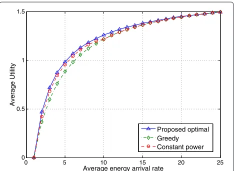
better than the greedy policy. For the Poisson distributed energy arrival (Figure 4), the greedy policy performs worse than the constant policy at low energy arrival rate regime (h¯ < 6), but better at high energy arrival rate regime (6 ≤ ¯h< 10). The performance converge to the optimal whenh¯ ≥ 10. In Figure 5, the behavior of these policies under Geometric distributed energy arrival is similar with the uniform distributed scenario. However, the two base-line policies in this scenario converge to the optimal much slower than in the uniform distributed scenario. At last, the performance under the binomial distributed energy arrival is illustrated in Figure 6, which is similar with the Poisson distributed case. To sum up, all the simulations show that the constant policy shows higher performance than the greedy policy in low energy arrival rate regime. However, there are still gaps to the optimal solution
Table 7 Policy comparison under different energy arrival distribution in high SNR regime with parameters
γ =10,h¯ =6,n=15
Battery state Unif. Poiss. Geom. Bin.
0 0 0 0 0
1 1 1 1 1
2 2 2 1 2
3 3 3 2 3
4 3 4 3 4
5 4 5 3 5
6 5 5 3 5
7 5 6 4 6
8 6 6 5 6
9 7 7 5 7
10 7 8 5 8
Table 8 Policy comparison under different energy arrival distribution in low SNR regime with parameters
γ =0.01,h¯ =6,n=15
Battery state Unif. Poiss. Geom. Bin.
0 0 0 0 0
1 1 1 1 1
2 2 2 2 2
3 3 3 3 3
4 4 4 4 4
5 5 5 5 5
6 6 6 6 6
7 7 7 7 7
8 8 8 8 8
9 9 9 9 9
10 10 10 10 10
(maximum of 10% gap under geometric distribution and maximum of 2% to 3% under the rest distributions).
6 Conclusions
In this paper, we analyzed the optimal power allocation policy under a discrete system model using the Markov chain analysis. We proved that the problem can be solved via linear programming approach and analyzed the prop-erties of the optimal policy. And for the greedy power allocation policy, we found the condition to guarantee its optimality. Numerical results show that under finite battery capacity condition, the optimal policy is quite different from that under infinite battery capacity con-dition. Specifically, different from the infinite battery case, the energy allocated in each slot might be larger
0 5 10 15
0.4 0.6 0.8 1 1.2 1.4 1.6 1.8
Average energy arrival rate
Average Utility
Proposed optimal Greedy Constant power
1 2 3 4 5 6 7 8 9 10 0.4
0.6 0.8 1 1.2 1.4 1.6 1.8 2
Average energy arrival rate
Average Utility
Proposed optimal Greedy Constant power
Figure 4The performance of the proposed optimal power allocation policy under Poisson distributed energy arrival with parameterγ=1.
than the average arrival rate. Also, extensive simulations showed the consistent results with the analysis for the greedy optimal condition. Based on the intuition provided through the analysis of discrete model, future work will extend our results to the continuous energy model sce-nario and the extensive wireless systems with multiple antennas/subcarriers.
Appendices Appendix 1 Proof of Theorem 1
We prove the theorem by contradiction. Notice thatπi∗> 0 means that stateiis not a transient state. Suppose for
0 5 10 15 20 25
0 0.5 1 1.5
Average energy arrival rate
Average Utility
Proposed optimal Greedy Constant power
Figure 5The performance of the proposed optimal power allocation policy under geometric distributed energy arrival with parameterγ =1.
1 2 3 4 5 6 7 8
0.4 0.6 0.8 1 1.2 1.4 1.6 1.8
Average energy arrival rate
Average Utility
Proposed optimal Greedy Constant power
Figure 6The performance of the proposed optimal power allocation policy under binomial distributed energy arrival with parameterγ=1,n=10.
non-transient statesi,m,p∗i,j > 0,p∗m,n > 0, wherem > i,n < j. We provide the proof in the following two cases separately.
1) If:
p∗m,n p∗i,j ≥
π∗ i π∗
m
, (39)
we construct a power allocation policy matrix P by setting:
pi,n = p∗i,n+p∗i,j, (40)
pi,j = 0, (41)
pm,n = p∗m,n− π ∗ i π∗
m
p∗i,j, (42)
pm,j = p∗m,j+ π ∗ i π∗
m
p∗i,j, (43)
andpk,l =p∗k,lfor the other elements. We have:
!
π∗"T
P = !π∗"TP∗, (44)
i
k=0
pi,k = 1, ∀i (45)
pi,j ≥ 0, ∀i≥j (46)
i.e., the power allocation policyPstill satisfies all the con-straints (9b), (9c), and (10), and the stationary distribution π∗does not change under the new policy. Hence, all the
(i,n),(i,j),(m,n),(m,j). For the clarity of comparison, we
Joint with (40)-(43), we can get:
D−D=πi∗p∗i,j(um−n−um−j)−(ui−n−ui−j)(<a)0, (49)
where (a) is due to the concavity of utility function. As a result, with the revised policyP, a larger average utility is obtained, which contradicts the optimality ofP∗.
2) If:
and following the same deduction procedure of case 1), we can obtain the same contradiction.
To sum up, with the assumption that for non-transient statesi,m,p∗i,j >0 andp∗m,n >0,m> i,n< j, it ends up thatP∗is not optimal. Hence, the theorem is proved with the contradiction.
Appendix 2 Proof of Theorem 2
The theorem can be proved according to the simplex method[19]. Specifically,fg = hT0, 0,. . ., 0T is a basic
feasible solution, and the resulting objective function is uT0h0.
Consider a feasible solution f = fT0,f1T,. . .,fTNT as initially defined in P-3M. From (19), we can get:
f0=h0+
Then, the objective value can be written as:
uTf=uT0f0+ of the utility functionuj, we have:
ci,k−ci,k−1=(uk−uk−1)−(uk+i−uk+i−1)≥0, ∀k.
where inequality (a) holds due to the concavity ofuj, (b)
is derived from (29), and (c) holds since hj ≥ 0 and uj is increasing. Combining (58) and (59), we can
con-clude thatc1,N−1is the largest element. Since c1,N−1 = N−1
i=0 hi(ui+1−ui)−uN−uN−1≤0, all the elements of ci,i= 1,. . .,Nis non-positive, and hence the optimality
Competing interests
The authors declare that they have no competing interests.
Authors’ contributions
The authors of the paper are of equal contribution to this paper. All authors read and approved the final manuscript.
Acknowledgements
This work is sponsored in part by the National Basic Research Program of China (No. 2012CB316001), and the Nature Science Foundation of China (No. 61201191 and 61401250), the Creative Research Groups of NSFC (No. 61321061), the Sino-Finnish Joint Research Program of NSFC
(No. 61461136004), and Hitachi R&D Headquarter.
Author details
1Tsinghua National Laboratory for Information Science and Technology,
Department of Electronic Engineering, Tsinghua University, 100084 Beijing, People’s Republic of China.2China Mobile Communication Corporation (CMCC), No. 29, Financial Street, Xicheng District, Beijing 100033, People’s Republic of China.
Received: 31 October 2014 Accepted: 9 February 2015
References
1. Ericsson,Sustainable energy use in mobile communications. (Ericsson Inc. white paper, 2007)
2. J Yang, S Ulukus, Optimal packet scheduling in an energy harvesting communication system. IEEE Trans. Commun.60(1), 220–230 (2012) 3. K Tutuncuoglu, A Yener, Optimum transmission policies for battery
limited energy harvesting nodes. IEEE Trans. Wireless Commun.11(3), 1180–1189 (2012)
4. O Ozel, K Tutuncuoglu, J Yang, S Ulukus, A Yener, Transmission with energy harvesting nodes in fading wireless channels: optimal policies. IEEE J. Selected Areas Commun.29(8), 1732–1743 (2011)
5. CK Ho, R Zhang, Optimal energy allocation for wireless communications with energy harvesting constraints. IEEE Trans. Signal Process.60(9), 4808–4818 (2012)
6. C Hu, J Gong, X Wang, S Zhou, Z Niu, inIEEE/CIC International Conference on Communications in China (ICCC). Spatial-temporal water-filling power allocation in MIMO systems with harvested energy, (2013), pp. 588–593 7. J Gong, S Zhou, Z Niu, Optimal power allocation for energy harvesting
and power grid coexisting wireless communication systems. IEEE Trans. Commun.61(7), 3040–3049 (2013)
8. J Xu, R Zhang, Throughput optimal policies for energy harvesting wireless transmitters with non-ideal circuit power. IEEE J. Selected Areas Commun. 32(2), 322–332 (2014)
9. C Huang, R Zhang, S Cui, Throughput maximization for the gaussian relay channel with energy harvesting constraints. IEEE J. Selected Areas Commun.31(8), 1469–1479 (2013)
10. V Sharma, U Mukherji, V Joseph, S Gupta, Optimal energy management policies for energy harvesting sensor nodes. IEEE Trans. Wireless Commun.9(4), 1326–1336 (2010)
11. DP Bertsekas,Dynamic Programming and Optimal Control, Volume II, 3rd edn. (Athena Scientific, Massachusetts, 2005)
12. CK Ho, R Zhang, inIEEE International Symposium on Information Theory Proceedings (ISIT). Optimal energy allocation for wireless communications powered by energy harvesters, (2010), pp. 2368–2372
13. BT Bacinoglu, E Uysal-Biyikoglu, Finite-horizon online transmission scheduling on an energy harvesting communication link with a discrete set of rates. J. Commun. Netw.16(3), 293–300 (2014)
14. PK Deekshith, V Sharma, R Rajesh, AWGN channel capacity of energy harvesting transmitters with a finite energy buffer. arXiv preprint, available online: http://arxiv.org/abs/1307.4505
15. L Huang, MJ Neely, Utility optimal scheduling in energy-harvesting networks. IEEE/ACM Trans. Netw. (TON).21(4), 1117–1130 (2013) 16. M Zheng, P Pawełczak, S Sta ´nczak, H Yu, Planning of cellular networks
enhanced by energy harvesting. arXiv preprint, available online: http://arxiv.org/abs/1304.5088
17. Y-K Chia, S Sun, R Zhang, inIEEE Wireless Communications and Networking Conference (WCNC). Energy cooperation in cellular networks with renewable powered base stations, (2013), pp. 2542–2547
18. TM Cover, JA Thomas,Elements of Information Theory. (John Wiley & Sons, New York, USA, 2012)
19. RJ Vanderbei,Linear Programming: Foundations and Extensions, 3nd edn. (Springer, Berlin, Germany, 2010)
20. V Klee, GJ Minty,How good is the simplex algorithm?(Academic Press, New York-London, 1972), pp. 159–175
Submit your manuscript to a
journal and benefi t from:
7Convenient online submission 7Rigorous peer review
7Immediate publication on acceptance 7Open access: articles freely available online 7High visibility within the fi eld
7Retaining the copyright to your article