No-signaling Linear PCPs

(1)

No-signaling Linear PCPs

Susumu Kiyoshima

NTT Secure Platform Laboratories [email protected]

January 18, 2019

Abstract

In this paper, we give a no-signaling linear probabilistically checkable proof (PCP) system for polynomial-time deterministic computation, i.e., a PCP system forPsuch that (1) the honest PCP oracle is a linear function and (2) the soundness holds against any (computational) no-signaling cheating prover, who is allowed to answer each query according to a distribution that depends on the entire query set in a certain way. To the best of our knowledge, our construction is the first PCP system that satisfies these two properties simultaneously.

As an application of our PCP system, we obtain a 2-message delegating computation scheme by using a known transformation. Compared with the existing 2-message delegating computation schemes that are based on standard cryptographic assumptions, our scheme requires preprocessing but has a simpler structure and makes use of different (possibly cheaper) standard cryptographic primitives, namely additive/multiplicative homomorphic encryption schemes.

This article is a full version of an earlier article: No-signaling Linear PCPs, in Proceedings of TCC 2018, ©IACR 2018,

(2)

1 Introduction

Linear PCP. Probabilistically checkable proofs, or PCPs, are proof systems with which one can probabilistically verify the correctness of statements with bounded soundness error by reading only a few bits/symbols of proof strings. A central result about PCPs are thePCP theorem[AS98,ALM+98], which states that everyNPstatement has a PCP system such that the proof string is polynomially long and the verification requires only a constant number of bits of the proof string (the soundness error is a small constant and can be reduced by repetition).

An important application of PCPs to Cryptography issuccinct argument systems, i.e., argument systems that have very small communication complexity and fast verification time. A famous example of such argument systems is that of Kilian [Kil92], which provesNP statements by using PCPs as follows.

1. The prover first generates a polynomially long PCP proof for the statement (this is possible thanks to the PCP theorem) and succinctly commits to it by using Merkle’s tree-hashing tech-nique.

2. The verifier queries a few bits of the PCP proof just like the PCP verifier.

3. The prover reveals the queried bits by appropriately opening the commitment using the local opening property of Merkle’s tree-hashing.

This argument system of Kilian has communication complexity and verification time that depend on the classical _NPverification time only logarithmically; that is, a proof for the membership of an instancexin anNPlanguageLhas communication complexity and verification timepoly(λ+|x|+ logt), whereλis the security parameter,tis the time to evaluate theNPrelation ofLon x, andpoly

is a polynomial that is independent ofL. Kilian’s technique was later extended to obtain succinct non-interactive argument systems (SNARGs) forNPin the random oracle model [Mic00] as well as in the standard model with non-falsifiable assumptions (such as the existence of extractable hash functions), e.g., [BCC+17,DFH12].1

Recently, a specific type of PCPs calledlinear PCPshas boosted the studies of succinct argument systems. Linear PCPs are PCPs such that the honest proofs are linear functions (i.e., the honest proof strings are the truth tables of linear functions).2 _{The proof strings of linear PCPs are usually} exponen-tially long, but each bit or symbol of them can be computed efficiently by evaluating the underlying linear functions. A nice property of linear PCPs is that they often have much simpler structures than the existing polynomially long non-linear PCPs; as a result, the use of linear PCPs often lead to sim-pler constructions of succinct argument systems. The use of linear PCPs in the context of succinct argument systems was initiated by Ishai, Kushilevitz, and Ostrovsky [IKO07], who used them for constructing an argument system forNP with a laconic prover (i.e., a prover that sends to the ver-ifier only short messages). Subsequently, several works obtained practical implementations of the argument system of Ishai et al. [SBW11,SMBW12,SVP+12, SBV+13,VSBW13], whereas others extended the technique of Ishai et al. for the use for SNARGs and obtained practical implementations ofpreprocessing SNARGs(i.e., SNARGs that require expensive (but reusable) preprocessing setups) [BCI+13,BCG+13,BCTV14].

1_{Actually, SNARGs in the standard model require the existence of common reference strings, and some constructions of}

them further require that the verifier has some private information about the common reference strings.

2_{In general, their soundness is required to hold against any (possibly non-linear) functions; linear PCPs with this notion}

(5)

No-signaling PCP. Very recently, Kalai, Raz, and Rothblum [KRR13, KRR14] found that PCPs with a stronger soundness guarantee, called soundness against no-signaling provers, are useful for constructing 2-message succinct argument systems under standard assumptions. Concretely, Kalai et al. [KRR13,KRR14] found that (1) no-signaling PCPs (i.e., PCPs that are sound against no-signaling provers) can be constructed for deterministic computation, and (2) their no-signaling PCPs can be used to obtain 2-message succinct argument systems for deterministic computation under the assumptions of the existence of quasi-polynomially secure fully homomorphic encryption schemes or (2-message, polylogarithmic-communication, single-server) private information retrieval schemes. The succinct argument systems of Kalai et al. differ from prior ones in that they can handle only deterministic com-putation but requires just two messages and is proven secure under standard assumptions. (In contrast, the argument system of Kilian and prior SNARG systems can handle non-deterministic computation but the former requires four messages and the latter are proven secure only in ideal models such as the random oracle model or under non-falsifiable knowledge-type assumptions.)

As observed by Kalai et al. [KRR13,KRR14], 2-message succinct argument systems have a direct application indelegating computation [GKR15] (orverifiable computation [GGP10]). Specifically, consider a setting where there exist a computationally weak client and a computationally powerful server, and the client wants to delegate a heavy computation to the server. Given a 2-message suc-cinct argument system, the client can delegate the computation to the server in such a way that it can verify the correctness of the server’s computation very efficiently (i.e., much faster than doing the computation from scratch).

After the results of Kalai et al. [KRR13, KRR14], no-signaling PCPs and their applications to delegation schemes have been extensively studied. Kalai and Paneth [KP16] extended the results of Kalai et al. [KRR14] and obtained a delegation scheme for deterministic RAM computation, and Brakerski, Holmgren, and Kalai [BHK17] further extended it so that the scheme is adaptively sound (i.e., sound even when the statement is chosen after the verifier’s message) and in addition can be based on polynomially hard standard cryptographic assumptions. Paneth and Rothblum [PR17] gave an adaptively sound delegation scheme for deterministic RAM computation with public verifiability (i.e., with a property that not only the verifier but also anyone can verify proofs) albeit with the use of a new cryptographic assumption. Badrinarayanan, Kalai, Khurana, Sahai, and Wichs [BKK+18] gave an adaptively sound delegation scheme for low-space deterministic computation (i.e., non-deterministic computation such that the space complexity is much smaller than the time complexity) under sub-exponentially hard cryptographic assumptions.

The no-signaling PCPs that are used by Kalai et al. [KRR13,KRR14] and the subsequent works are not linear. As a result, compared with the delegation schemes that are obtained from the linear-PCP– based preprocessing SNARGs [BCI+13,BCG+13,BCTV14], their delegation schemes have complex structures.

1.1 Our Results

(6)

Main Result: No-signaling linear PCP forP. The main result of this paper is an unconditional construction of no-signaling linear PCPs for polynomial-time deterministic computation. Our con-struction is designed for proving correctness of arithmetic circuit computation, so it handles statements of the form(C,x,y), whereCis a polynomial-size arithmetic circuit and the statement to be proven is “C(x)=yholds.”

Theorem(informal). There exists a no-signaling linear PCP for the correctness of polynomial-size arithmetic circuit computation. For a statement(C,x,y) and the security parameter1λ, the proof generation algorithm runs in timepoly(|C|), the verifier query algorithm runs in timepoly(λ+|C|), and the verifier decision algorithm runs in timepoly(λ+|x|+|y|).

A formal statement of this theorem is given asTheorem 1inSection 4. To the best of our knowledge, our construction is the first linear PCP that is sound against no-signaling provers. (SeeSection 1.3for concurrent independent works.)

Our no-signaling linear PCP has a simple structure just like the existing linear PCPs. Indeed, the proof string of our PCP is identical with that of the well-known linear PCP of Arora, Lund, Motwani, Sudan, and Szegedy [ALM+98]. Regarding the verifier, we added slight modifications to that of Arora et al. to simplify the analysis; however, we do not think that these modifications are fundamental.

The analysis of our no-signaling linear PCP is a combination of the analysis of the linear PCP of Arora et al. [ALM+98] and that of the no-signaling PCP of Kalai et al. [KRR14]. Specifically, our analysis on no-signaling soundness follows the same high-level strategy as that of Kalai et al. while borrowing techniques from Arora et al. for implementing the details of the strategy. Additionally, our analysis is simplified from the analysis of Kalai et al. in the sense that, while the analysis of Kalai et al. requires the circuitCin the statement to have a specific redundant form called “augmented layered circuit,” our analysis only requiresCto have a much less redundant form called “layered circuit.” (This simplification relies on a specific structure of our PCP.) A more detailed overview of our analysis is given inSection 3.

Application: Delegation scheme forPin the preprocessing model. As an application of our no-signaling linear PCP, we construct a 2-message delegation scheme for polynomial-time deterministic computation under standard cryptographic assumptions. Just like previous linear-PCP–based dele-gation schemes and succinct arguments (such as that of Bitansky et al. [BCI+13]), our delegation scheme works in thepreprocessing model, so our scheme requires expensive offline setups that can be reused for proving multiple statements. When the statement is(C,x,y), the running time of the client ispoly(λ+|C|)in the offline phase and ispoly(λ+|x|+|y|)in the online phase. Our delega-tion scheme is adaptively secure in the sense that the inputxcan be chosen in the online phase, and is “designated-verifier type” in the sense that the verification requires a secret key. We obtain our delega-tion scheme by applying the transformadelega-tion of Kalai et al. [KRR13,KRR14] on our no-signaling liner PCP. (The transformation of Kalai et al., which is closely related to those of Biehl, Meyer, and Wetzel [BMW98] and Aiello, Bhatt, Ostrovsky, and Rajagopalan [ABOR00], transforms a no-signaling PCP to a 2-message delegation scheme.)

(7)

prime-order fields (such as that of Goldwasser and Micali [GM84]) or multiplicative homomorphic encryp-tion schemes over prime-order bilinear groups (such as the DLIN-based linear encrypencryp-tion scheme of Boneh, Boyen, and Shacham [BBS04]).

1.2 Prior Works

Delegation scheme. Delegation schemes (and verifiable computation schemes) have been exten-sively studied in literature. Other than those that we mentioned above, existing results that are related to ours are the following. (We focus our attention on non-interactive or 2-message delegation schemes for all deterministic or non-deterministic polynomial-time computation.)

Delegation schemes for non-deterministic computation. The existing constructions of

(prepro-cessing) SNARGs, such as [Gro10, Lip12, DFH12, BC12, GGPR13, BCI+13, BCCT13, Lip13,

DFGK14,Gro16,BISW17,BCC+17], can be directly used to obtain delegation schemes forNP, and some of them can be used even to obtain publicly verifiable ones. Additionally, it was shown recently that an interactive variant of PCPs, calledinteractive oracle proofs, can also be used to obtain dele-gation schemes forNP[BCS16]. The security of these delegation schemes holds under non-standard assumptions (e.g., knowledge assumptions) or in ideal models (e.g., the generic group model and the random oracle model). Compared with these schemes, our scheme works only for_Pand requires pre-processing, but can be proven secure in the standard model under a standard assumption (namely the existence of homomorphic encryption schemes).

Delegation schemes for deterministic computation. Other than the abovementioned recent works that obtain delegation schemes forPby using no-signaling PCPs (i.e., Kalai et al. [KRR13, KRR14] and the subsequent works), there are plenty of works that obtain delegation schemes for

Pwithout using PCPs. Specifically, some works obtain schemes with preprocessing by using fully homomorphic encryption or attribute-based encryption schemes [GGP10,CKV10,PRV12], and oth-ers obtain schemes without preprocessing by using multi-linear maps or indistinguishability obfusca-tors (e.g., [BGL+15,CHJV15,CH16,CCHR16,KLW15,CCC+16,ACC+16]). Compared with these schemes, our scheme requires preprocessing but only uses relatively simple building blocks (namely a linear PCP and a homomorphic encryption scheme).

1.3 Concurrent Works

In independent concurrent works, Holmgren and Rothblum [HR18] and Chiesa, Manohar, and Shinkar [CMS19] also observe that one can obtain no-signaling PCPs for_Pwithout relying on the “augmented circuit” technique of Kalai et al. [KRR14]. The technique by Holmgren and Rothblum works when the underlying PCP is that of Babai et al. [BFLS91] (as in the work of Kalai et al. [KRR14]) and the one by Chiesa et al. works when the underlying PCP is that of Arora et al. [ALM+98] (as in this paper).

Actually, the work of Chiesa et al. [CMS19] has many other similarities with our work, and in particular their work shows that the linear PCP of Arora et al. [ALM+98] is sound against no-signaling cheating provers. Differences between their work and our work include:

• Chiesa et al. achieve constant soundness error with constant query complexity while we focus on achieving negligible soundness error and did not try to optimize the query complexity (specifi-cally, we slightly modified the verifier algorithm, and our analysis currently requires polynomial query complexity3_).

(8)

• The analysis by Chiesa et al. uses the equivalence between no-signaling functions and quasi-distributions4 _{over functions while ours does not use this equivalence. (The equivalence} be-tween no-signaling functions and quasi-distributions was shown by Chiesa, Manohar, and Shinkar [CMS18] relying on Fourier analytic techniques.)

Remark1. Chiesa et al. [CMS19] use the term “no-signaling linear PCPs” in a different meaning from us. Specifically, Chiesa et al. use it to refer to PCPs such that the honest proofs are linear functions and the soundness holds against no-signaling cheating provers that are equivalent with quasi-distributions over linear functions, while we use it to refer to PCPs such that the honest proofs are linear func-tions and the soundness holds againstanyno-signaling cheating provers (which are not necessarily equivalent with quasi-distributions over linear functions).

1.4 Outline

InSection 2, we introduce the notations and definitions that we use in the subsequent sections. In Section 3, we give an overview of the construction and analysis of our no-signaling linear PCP. In Section 4, we formally describe the construction of our no-signaling linear PCP. FromSection 5to Section 9, we analyze the no-signaling soundness of our construction. InSection 10, we describe the application to delegation schemes.

2 Preliminaries

In this section, we introduce the notations and definitions that we use in the subsequent sections.

2.1 Basic Notations

We denote the security parameter byλ. LetNbe the set of all natural numbers. For anyk ∈ N, let

[k]B{1, . . . ,k}.

We denote a vector in a bold shape (e.g.,v). For a vectorv = (v1, . . . ,v_λ)and a setS ⊆ [λ], let

v|S B {vi}i∈S. Similarly, for a function f : D → R and a setS ⊆ D, let f|S B {f(i)}i∈S. For two

vectorsu= (u1, . . . ,u_λ),v= (v1, . . . ,v_λ)of the same length (where each element is a field element), let⟨u,v⟩B∑_i_∈_[_λ_]uividenote their inner product andu⊗vB(uivj)i,j∈[λ]denote their tensor product.5

For a setS, we denote bys←S a process of obtaining an elements∈S by a uniform sampling fromS. Similarly, for any probabilistic algorithmAlgo, we denote byy←Algoa process of obtaining an outputyby an execution of Algowith uniform randomness. For an event E and a probabilistic processP, we denote byPr [E|P]the probability ofEoccuring over the randomness ofP.

2.2 Circuits

All circuits in this paper are arithmetic circuits over finite fields of prime orders, and they have addition and multiplication gates with fan-in 2. We assume without loss of generality that they are “layered,” i.e., the gates in a circuit can be partitioned into layers such that (1) the first layer consists of the input

formally.

4_{Quasi-distributions are a generalized notion of probability distributions and allow negative probabilities.}

5_{In this paper, the tensor product of two vectors are viewed as a vector (with an appropriate ordering of the elements)}

(9)

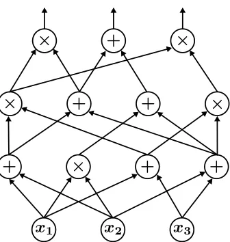
Figure 1: A layered circuit, where the gates in the bottom layer are the input gates and those in the top layer are the output gates.

gates and the last layer consists of the output gates, and (2) the gates in thei-th layer have children in the(i−1)-th layer (seeFigure 1for an illustration).

Given a circuitC, we use_Fto denote the underlying finite field, N to denote the number of the wires,6 n to denote the number of the input gates, andmto denote the number of the output gates. We assume that the firstn wires ofC are those that take the values of the input gates and the last

mones are those that take the value of the output gates. (Formally, _F_,N,n,mshould be written as, e.g.,FC,NC,nC,mC since they depend on the circuitC. However, to simplify the notations, we avoid

expressing this dependence.) When we consider a circuit family{C_λ}_λ∈_N, it is implicitly assumed that the size of eachC_λis bounded bypoly(λ).

2.3 Probabilistically Checkable Proofs (PCPs)

Roughly speaking, probabilistically checkable proofs (PCPs) are proof systems with which one can probabilistically verify the correctness of statements by reading only a few bits or symbols of the proof strings. A formal definition is given below.

Remark2 (On the definition that we use). For convenience, we give a definition that is tailored to our purpose. Specifically, our definition differs from the standard one in the following way.

1. We require that the soundness error is negligible in the security parameter.

2. We only consider proofs for the correctness of deterministic arithmetic circuit computation, i.e., membership proofs for the following language.

{(C,x,y)|Cis an arithmetic circuit s.t.C(x)= y} .

3. We implicitly require that PCP systems satisfy two auxiliary properties (which almost all exist-ing constructions satisfy), namelyrelatively efficient oracle construction andnon-adaptive verifier[BG09].

(10)

4. We assume that the verifier’s queries depend only on the circuitCand do not depend on the input

xand the output y. (This assumption will be useful later when we define adaptive soundness

against no-signaling cheating provers.) ^

Definition 1(PCPs for correctness of arithmetic circuit computation). A probabilistically checkable

proof (PCP) system for the correctness of arithmetic circuit computationconsists of a pair of ppt

Turing machinesV =(V0,V1)(calledverifier) and a ppt Turing machineP(calledprover) that satisfy the following.

• Syntax. For every arithmetic circuitC, there exist

– finite setsDC andΣC(calledproof domainandproof alphabet) and – a polynomialκV (calledquery complexityofV)

such that for every inputxofC, the outputyBC(x), and every security parameterλ∈N, – P(C,x)outputs a functionπ:DC →ΣC(calledproof),

– V0(1λ,C)outputs a stringstV ∈ {0,1}∗(calledstate) and a setQ⊂DCof sizeκV(λ)(called

queries), and

– V1(stV,x,y, π|Q)outputs a bitb∈ {0,1}.

• Completeness. For every arithmetic circuitC, every input xofC, the output y B C(x), and

every security parameterλ∈N,

Pr

[

V1(stV,x,y, π|Q)=1 π←

P(C,x)

(Q,stV)←V0(1λ,C)

]

=1 .

• Soundness. For any circuit family{C_λ}_λ∈_Nand any probabilistic Turing machine P∗ (called

cheating prover), there exists a negligible functionneglsuch that for every security parameter λ∈N,

Pr

[

V1(stV,x,y, π∗|Q)=1∧Cλ(x), y

(Q,stV)←V0(1λ,C_λ) (x,y, π∗)←P∗(1λ,C_λ)

]

≤negl(λ) .

^

A PCP system is said to be linear if the honest proof is a linear function.

Definition 2(Linear PCPs). Let(P,V)be any PCP system and {DC}C be its proof domains. Then, (P,V)is said to belinearif for every arithmetic circuitCand inputxofC,

Pr

   ∧

u,v∈DC

π(u)+π(v)=π(u+v)

(11)

2.4 No-signaling PCPs

No-signaling PCPs [KRR13,KRR14] are PCP systems that guarantee soundness against a stronger class of cheating provers called signaling cheating provers. The main difference between no-signaling cheating provers and normal cheating provers in that, while a normal cheating prover is required to output a PCP proof_π∗before seeing queriesQ, a no-signaling cheating prover is allowed to outputπ∗after seeingQ. There is however a restriction on the distribution ofπ∗; roughly speaking, it is required that for any (not too large) setsQ,Q′such thatQ′⊂Q, the distribution ofπ∗|Q′ when the

queries areQshould be indistinguishable from the distribution of it when the queries areQ′. The for-mal definition is given below. (The following definition is the computational variant of the definition, which is given by Brakerski, Holmgren, and Kalai [BHK17].)

Definition 3(No-signaling cheating prover). Let(P,V)be any PCP system,{DC}C and{ΣC}C be the proof domains and proof alphabets of(P,V),{C_λ}_λ∈_Nbe any circuit family, andP∗be any probabilistic Turing machine with the following syntax.

• Given the security parameterλ∈N, the circuitC_λ, and a set of queriesQ⊂ DC_λas input,P∗ outputs an input xofC_λ, an outputyofC_λ, and a partial function_π∗:Q→ΣCλ. (Note thatπ∗ can be viewed as a PCP proof whose domain is restricted toQ.)

Then, for any polynomial_κmax, P∗is said to be a_κmax-wise (computational) no-signaling cheating

proverif for any ppt Turing machine D, there exists a negligible function neglsuch that for every

λ∈N, everyQ,Q′⊂ DC_λsuch thatQ′⊂ Qand|Q| ≤κmax(λ), and everyz∈ {0,1}poly(λ),

Pr[D(C_λ,x,y, π∗|Q′,z)=1 (x,y, π∗)←P∗(1λ,Cλ,Q)

]

−Pr[D(C_λ,x,y, π∗,z)=1 (x,y, π∗)←P∗(1λ,C_λ,Q′) ]

≤negl(λ) .

^

Now, we define no-signaling PCPs as the PCP systems that satisfy soundness according to the following definition.

Definition 4(Soundness against no-signaling cheating provers). Let(P,V)be any PCP system andκmax be any polynomial. Then,(P,V)is said to besound against_κmax-wise (computational) no-signaling cheating proversif for any circuit family{C_λ}_λ∈_Nandκmax-wise no-signaling cheating proverP∗, there exists a negligible functionneglsuch that for everyλ∈N,

Pr

[

V1(stV,x,y, π∗)=1∧C_λ(x), y (Q,stV)←V0(1

λ_,_C λ) (x,y, π∗)←P∗(1λ,C_λ,Q)

]

≤negl(λ) .

^

3 Technical Overview

(12)

underlying finite field, N to denote the number of the wires,7 n to denote the number of the input gates, andmto denote the number of the output gates. We assume that the firstnwires are those that take the values of the input gates and the lastmones are those that take the value of the output gates. In this overview, we additionally assume that the output length is1(i.e.,m=1).

3.1 Preliminary: Linear PCP of Arora et al. [ALM+98]

The construction and analysis of our PCP system is based on the linear PCP system of Arora et al. [ALM+98] (ALMSS linear PCP in short), so we start by recalling it. We only describe the construction of ALMSS linear PCP in this section; a more detailed overview of ALMSS linear PCP can be found inAppendix A.

3.1.1 Main tool: Walsh–Hadamard code.

The main tool of ALMSS linear PCP system is Walsh–Hadamard code. Recall that Walsh–Hadamard code maps a stringv ∈ Fℓ to the linear functionWHv : x 7→ ⟨v,x⟩. A useful property of Walsh– Hadamard code is that errors on codewords can be easily “self-corrected.” In particular, if a function

f :Fℓ→Fisδ-closeto a linear function _fˆ_{(i.e., if there exists a linear function} _fˆ_{such that}_Pr[_f_(r)₌ ˆ

f(r)|r←Fℓ]≥δ), we can evaluate _fˆ_{on any point}_x_∈_Fℓ_{with error probability}₂₍₁₋_δ)_{through the} following simple probabilistic procedure.

AlgorithmSelf-Correctf(x):

Choose random r∈Fℓand output f(x+r)− f(r).

3.1.2 Construction of ALMSS linear PCP.

On input(C,x), the proverPcomputes the PCP proof as follows. First, Pcomputesy B C(x)and obtains the following system of quadratic equations overF, which is designed so that it is satisfiable if and only ifC(x)=y.

• The variables arez=(z1, . . . ,zN).

• For eachi∈ {1, . . . ,n}, the system has the equationzi = xi.

• For eachi,j,k ∈[N], the system haszi+zj−zk = 0ifChas an addition gate with input wires i,jand output wirek, and haszizj−zk = 0ifChas a multiplication gate with input wiresi,j

and output wirek.

• The system has the equationzN =y.

(Intuitively, the variables of the above system of quadratic equations represent the wire values ofC, and the equations guarantee that (1) the correct input valuesx=(x1, . . . ,xn)are assigned on the input

gates, (2) each gate is correctly computed, and (3) the claimed output valueyis assigned on the output gate.) Let us denote the above system of quadratic equations byΨ ={Ψi(z)=ci}i∈[M], whereMis the

number of the equations. Then,Pobtains the satisfying assignmentw = (w1, . . . ,wN)ofΨthrough

the wire values ofConx, and outputs the two linear functionsπf(v)B⟨v,w⟩andπg(v′)B⟨v′,w⊗w⟩

as the PCP proof.8 _{(In short, the PCP proof is Walsh–Hadamard encodings of}_w_and_w_⊗_w_.)

7_{We assume that for any gate with fan-out more than one, all the output wires of that gate share the same index}_i_∈_[_N_]. 8_Formally,_P_{outputs a single linear function (with which the verifier can evaluate both}_π

(13)

Next, on input(C,x,y), the verifierVverifies the PCP proof as follows. First,Vobtains the system of quadratic equations_{Ψ =} _{_Ψi(z) = ci}i∈[M]. Next,V applies the following three tests on the PCP

proofλtimes in parallel.

1. (Linearity Test.)Choose random pointsr1,r2∈FNandr′₁,r′₂∈FN

2

and checkπf(r1)+πf(r2) ?

=

πf(r1+r2)andπg(r′₁)+πg(r′₂) ?

=πg(r′

1+r′2).

2. (Tensor-Product Test.) Choose two random pointsr1,r2∈FN, runar1 ←Self-Correct πf_(r

1), ar2 ←Self-Correct

πf_(r

2),ar1⊗r2 ←Self-Correct πg_(r

1⊗r2), and checkar1ar2

?

=ar1⊗r2.

3. (SAT Test.) Choose a random pointσ = (σ1, . . . , σM) ∈ FM_{, compute a quadratic function}

Ψσ(z) B ∑_iM₌₁σiΨi(z), run a_ψ_σ ← Self-Correctπf₍ψ

σ), a_ψ′

σ ← Self-Correctπg(ψ′σ) for the

coefficient vectors_ψ_σ_,_ψ′_σsuch that_⟨_ψ_σ_,z⟩+⟨ψ′_σ,z⊗z⟩= Ψσ(z), and checka_ψ_σ +a_ψ′

σ

?

=c_σ, wherec_σB∑_iM₌₁σici.

V accepts the proof if it passes the above three tests in all theλparallel trials. It can be verified by inspection that, as required inDefinition 1, the verifier can be decomposed intoV0andV1, whereV0

samples the queries to the tests andV1 verifies the answers from the PCP proof. (Note thatV0 can

sample all the queries before knowingxandysince the coefficient vectorsψ_σ,ψ′_σin SAT Test can be computed fromCalone.)

3.2 Construction of Our No-signaling Linear PCP

The construction of our PCP system,(P,V), is essentially identical with that of ALMSS linear PCP. There is a slight difference in the verifier algorithm (in our PCP system,Self-Correctsamples many candidates of the self-corrected values and takes the majority), but we ignore this difference in this overview. It can be verified by inspection that the running time ofPispoly(|C|), the running time of

V0ispoly(λ+|C|), and the running time ofV1ispoly(λ+|x|+|y|).

3.3 Analysis of Our No-signaling Linear PCP

Our goal is to show that our PCP system(P,V)is sound against_κmax-wise no-signaling cheating provers for sufficiently large polynomialκmax. That is, our goal is to show that for every circuit family{C_λ}_λ∈_N

and everyκmax-wise no-signaling cheating proverP∗, we have

Pr

[

V1(stV,x,y, π∗)=1

∧C_λ(x),y

(Q,stV)←V0(1λ,Cλ) (x,y, π∗₎_←_P∗₍₁λ_,_C_λ_,_Q)

]

≤negl(λ) (3.1)

for every_λ_∈_N.

Toward this goal, for any sufficiently largeκmaxand anyκmax-wise no-signaling cheating prover

P∗, we assume that we have

Pr

[

(Q,stV)←V0(1λ,C_λ) (x,y, π∗)←P∗(1λ,C_λ,Q)

]

≥ _poly(λ)1 (3.2)

for infinitely manyλ∈N(letΛbe the set of thoseλ’s) and show that we have

Pr

[

C_λ(x),y (Q,stV)←V0(1

λ_,_C_λ₎

(x,y, π∗)←P∗(1λ,C_λ,Q)

]

(14)

for every sufficiently largeλ∈ Λ. Clearly, showing Equation (3.3) while assuming Equation (3.2) is sufficient for showing Equation (3.1) (this is because it implies that for every polynomialpolyand every sufficiently largeλ∈N, we haveV1(stV,x,y, π∗)= 1∧Cλ(x) ,ywith probability at most1/poly(λ)

since we either haveV1(stV,x,y, π∗) = 1with probability at most1/poly(λ) or haveCλ(x) , ywith

probability at most1/poly(λ)).

To explain the overall structure of our analysis, we first show Equation (3.3) while assuming the following (strong) simplifying assumptions instead of Equation (3.2).

Simplifying Assumption 1. P∗convinces the verifierV with overwhelming probability. That is, we have

Pr

[

(Q,stV)←V0(1λ,Cλ) (x,y, π∗)←P∗(1λ,C_λ,Q)

]

≥1−negl(λ) (3.4)

for infinitely manyλ ∈ N. (In what follows, we override the definition ofΛand let it be the set of

theseλ’s.) ^

Simplifying Assumption 2. P∗creates a proof that passes each of Linearity Test, Tensor-Product Test, and SAT Teston any pointswith overwhelming probability. That is, for every sufficiently largeλ∈Λ, we have the following. (We assume without loss of generality thatP∗ always outputs a PCP proof

π∗₌_(π∗

f, π∗g)that consists of two functionsπ∗f andπ∗g.)

• (Linearity of_π∗_f.)For everyu,v∈FN,

Pr[π∗_f(u)+π∗_f(v)=π∗_f(u+v)(x,y, π∗)←P∗(1λ,C_λ,{u,v,u+v})]≥1−negl(λ) , (3.5)

• (Linearity ofπ∗_g.)For everyu,v∈FN2_,

Pr[π∗_g(u)+π∗_g(v)=π∗_g(u+v)(x,y, π∗)←P∗(1λ,C_λ,{u,v,u+v})]≥1−negl(λ) , (3.6)

• (Tensor-Product Consistency ofπ∗_f, π∗_g.)For everyu,v∈FN_,

Pr[π∗_f(u)π∗_f(v)=π_g∗(u⊗v)(x,y, π∗)←P∗(1λ,C_λ,{u,v,u⊗v})]≥1−negl(λ) , (3.7)

• (SAT Consistency of_π∗_f_{, π}∗_g.)For everyσ∈FM_,

Pr[π∗_f(ψ_σ)+π∗_g(ψ′_σ)=c_σ (x,y, π∗)←P∗(1λ,C_λ,{ψ_σ,ψ′_σ})]≥1−negl(λ) . (3.8)

^

At the end of this subsection, we explain how we remove these simplifying assumptions in the actual analysis.

Under the above two simplifying assumptions, we obtain Equation (3.3) as follows. Notice that when the statement is true and the PCP proof is correctly generated, the first part of PCP proof,_πf(v)=

⟨v,w⟩, is the linear function whose coefficient vector is the satisfying assignmentwof the system of equationsΨ ={Ψi(z)=ci}i∈[M], and thus the satisfying assignment on any variablezican be recovered

by appropriately evaluatingπf. (Concretely, givenπf, we can obtain the satisfying assignment onzi

by evaluatingπf onei = (0, . . . ,0,1,0, . . . ,0) ∈ FN, where only thei-th element ofei is1). Now,

(15)

1. The assignment onzN (which represents the value of the output gate) is equal to the claimed output valuey. That is, for every sufficiently large_λ_∈_Λ,

Pr[π∗_f(eN)=y(x,y, π∗)←P∗(1λ,C_λ,{eN})

]

≥1−negl(λ) . (3.9)

2. The assignment onzN is equal to the actual output valueCλ(x). That is, for every sufficiently

largeλ∈Λ,

Pr[π∗_f(eN)=Cλ(x)(x,y, π∗)←P∗(1λ,Cλ,{eN})

]

≥1−negl(λ) . (3.10)

Indeed, given Equations (3.9) and (3.10), we can easily obtain Equation (3.3) as follows: first, we obtain

Pr[C_λ(x)=y(x,y, π∗)←P∗(1λ,C_λ,{eN})

]

≥1−negl(λ)

by applying the union bound on Equations (3.9) and (3.10); then, we obtain Equation (3.3) by using the no-signaling property of P∗ to argue that the probability ofC_λ(x) = y holding decreases only negligibly when the queries toP∗are changed from_{eN}to_{eN} ∪Qand from_{eN} ∪QtoQ.9 _(In this argument, we rely on the fact that the distinguisher in the no-signaling game can checkC_λ(x)=? y

efficiently.) Therefore, to conclude the analysis (under the simplifying assumptions), it remains to prove Equations (3.9) and (3.10).

3.3.1 Step 1. Showing consistency with the claimed computation.

First, we explain how we obtain Equation (3.9) under the simplifying assumptions onP∗.

To obtain Equation (3.9), we actually prove a stronger claim on the cheating assignment. Recall that from the construction of_{Ψ =}_{_Ψ_i(z) = ci}i∈[M], each equation ofΨis defined with at most three

variables, and in particular each equationΨi(z)=cican be written as

∑

j∈{α,β,γ} djzj+

∑

j,k∈{α,β,γ}

dj,kzjzk =ci

for someα, β, γ∈[N](α < β < γ),dj ∈ {−1,0,1}(j∈ {α, β, γ}), anddj,k ∈ {−1,0,1}(j,k ∈ {α, β, γ}).

Then, we consider the following claim.

1′. (Consistency with Claimed Computation)For anyi∈[M]and_{α, β, γ}_∈[N](_{α < β < γ}) such that the equationΨi(z)=cican be written as

∑

j∈{α,β,γ} djzj+

∑

j,k∈{α,β,γ}

dj,kzjzk =ci

for some dj ∈ {−1,0,1} (j ∈ {α, β, γ}) and dj,k ∈ {−1,0,1} (j,k ∈ {α, β, γ}), the cheating

assignment onz_α,z_β,z_γis a satisfying assignment of this equation. That is, for every sufficiently large_λ_∈_Λand everyiand_{α, β, γ}as above, we have

Pr[Consist_i(C_λ,x,y, π∗)(x,y, π∗)←P∗(1λ,C_λ,{e_α,e_β,e_γ})]≥1−negl(λ) , (3.11) whereConsist_i(C_λ,x,y, π∗)is the event that we have

∑

j∈{α,β,γ}

djπ∗_f(ej)+

∑

j,k∈{α,β,γ}

dj,kπ∗f(ej)π∗f(ek)=ci .

9_{We assume}_κ

(16)

Clearly, this claim implies Equation (3.9) sinceΨhas the equationzN =y.

Hence, we focus on showing the stronger claim that Equation (3.11) holds. Fix any sufficiently largeλ∈Λand anyi∈[M]. Assume for concreteness that the equationΨi(z) =cican be written as

−z_γ+z_αz_β=0. (The other cases can be proven similarly.) Under this assumption, our goal is to show

Pr[−π∗_f(e_γ)+π∗_f(e_α)π∗_f(e_β)=0(x,y, π∗)←P∗(1λ,C_λ,{e_α,e_β,e_γ})]≥1−negl(λ) . (3.12) First, we obtain

Pr[π∗_f(−e_γ)+π_g∗(e_α⊗e_β)=0(x,y, π∗)←P∗(1λ,C_λ,{−e_γ,e_α⊗e_β})]≥1−negl(λ) (3.13) by considering_σ₌ei∈FMin the SAT consistency of_π∗_f_{, π}∗_g(Equation (3.8) ofSimplifying Assump-tion 2). Second, we obtain

Pr[π∗_f(−e_γ)=−π∗_f(e_γ)(x,y, π∗)←P∗(1λ,C_λ,{e_γ,−e_γ})]≥1−negl(λ) (3.14) as a corollary of the linearity of_π∗_f (Equations (3.5) ofSimplifying Assumption 2),10_{and obtain}

Pr[π∗_g(e_α⊗e_β)=π∗_f(e_α)π∗_f(e_β)(x,y, π∗)←P∗(1λ,C_λ,{e_α,e_β,e_α⊗e_β})]≥1−negl(λ) (3.15) from the tensor-product consistency ofπ∗_f, π∗_g (Equation (3.7) ofSimplifying Assumption 2). Now, we obtain Equation (3.12) as desired from Equations (3.13), (3.14), (3.15), the union bound, and the no-signaling property ofP∗.11

3.3.2 Step 2. Showing consistency with the actual computation.

Next, we explain how we obtain Equation (3.10) under the simplifying assumptions onP∗.

Recall that, without loss of generality, we assume that arithmetic circuits are “layered,” i.e., the gates in a circuit can be partitioned into layers such that (1) the first layer consists of the input gates and the last layer consists of the output gate, and (2) the gates in thei-th layer have children in the

(i−1)-th layer.

The overall strategy is to prove Equation (3.10) by induction on the layers. For any circuitC_λ, let us use the following notations.

• ℓmaxis the number of the layers, and Niis the number of the wires in layeri(i.e., the number of the outgoing wires from the gates in layeri). We assume that the numbering of the wires are consistent with the numbering of the layers, i.e., the firstN1wires are those that are in the first

layer, the nextN2wires are those that are in the second layer, etc. • D1, . . . ,D_ℓmax are the subset ofF

N _{such that for every}_ℓ_∈_[_ℓmax_]_,

D_ℓB{v=(v1, . . . ,vN)|vi =0for∀i<{N≤ℓ−1+1, . . . ,N≤ℓ−1+Nℓ}} ,

where N_≤ℓ−1 B ∑i∈[ℓ−1]Ni. Notice that when the first part of the correct PCP proof,πf(v) =

⟨v,w⟩, is evaluated onv_ℓ ∈D_ℓ, it returns a linear combination of the correct wire values of layer

ℓ.

10_{Concretely, we first obtain}_Pr[_π∗

f(0)=0|(x,y, π∗)←P∗(1λ,Cλ,{0}) ]

≥1−negl(λ)from the linearity ofπ∗_f and then obtains Equation (3.14).

11_{To use the union bound on Equations (3.13), (3.14), (3.15), we need to argue that every probability in these equations}

does not decrease non-negligibly when we obtainπ∗_{by querying}_{_e_α,_e_β,_e_γ,₋_e_γ,_e

(17)

Now, to prove Equation (3.10), we show that the following three claims holds for every sufficiently large_λ_∈_Λ.

1. The cheating PCP proof is equal to the correct PCP proof on randomλpoints inD1. That is,

Pr U1,π∗

  ∧

u∈U1

π∗

f(u)=πf(u)

 

≥1−negl(λ) , (3.16)

where the probability is taken over u1,i ← D1 (i ∈ [λ]), U1 B {u1,i}i∈[λ], and (x,y, π∗) ← P∗(1λ,C_λ,U1), and_πf is the correct PCP proof that is generated by_π_BP(C_λ,x).

2. For everyℓ∈[ℓmax], if the cheating PCP proof is equal to the correct PCP proof on randomλ points inD_ℓ, the former is actually equal to the latter onanypoint inD_ℓ. That is, for anyv∈D_ℓ,

Pr

v,U_ℓ,π∗

 

π∗f(v)=πf(v)

∧

u∈U_ℓ π∗

f(u)=πf(u)

 

≥1−negl(λ) , (3.17)

where the probability is taken over u_ℓ,i ← Dℓ (i ∈ [λ]), Uℓ B {uℓ,i}i∈[λ], and (x,y, π∗) ← P∗(1λ,C_λ,{v} ∪U_ℓ).

3. For everyℓ∈[ℓmax−1], if the cheating PCP proof is equal to the correct PCP proof on random

λpoints inD_ℓ, the former is also equal to the latter equal on randomλpoints inD_ℓ+1. That is,

Pr Uℓ,Uℓ+1,π∗

   ∧

u∈Uℓ+1

π∗f(u)=πf(u)

∧

u∈Uℓ

π∗f(u)=πf(u)

 

≥1−negl(λ) , (3.18)

where the probability is taken overu_ℓ,i←Dℓ(i∈[λ]),uℓ+1,i←Dℓ+1(i∈[λ]),UℓB{uℓ,i}i∈[λ], U_ℓ+1 B{uℓ+1,i}i∈[λ], and(x,y, π∗)←P∗(1λ,Cλ,Uℓ∪Uℓ+1).

Observe that we can indeed obtain Equation (3.10) from the above three claims since Equation (3.17) implies that we can obtain Equation (3.10) by just showing

Pr Uℓmax,π∗

   ∧

u∈Uℓmax

π∗f(u)=πf(u)

 

≥1−negl(λ)

(this is because we haveπf(eN)=Cλ(x)from the construction of our PCP system), and we can obtain

this inequation by repeatedly using Equation (3.18) on top of Equation (3.16).12 Thus, what remain to prove are Equations (3.16), (3.17), (3.18).

1. First, we obtain Equation (3.16) from the linearity ofπ∗_f (Equations (3.5) of Simplifying As-sumption 2) and the consistency with the claimed computation (Equation (3.11) in Step 1) as follows. At a very high level, we first reduce the problem of showing Equation (3.16) to the problem of showing

∀i∈[n]: Pr[π∗_f(ei)=πf(ei)(x,y, π∗)←P∗(1λ,C_λ,{ei})]≥1−negl(λ)

12_{Formally, we need to argue that the probabilities in these inequations do not decrease non-negligibly when we change}

(18)

by relying on the linearity of π∗_f (the key point on this reduction is that any v ∈ D1 can be written as a linear combination ofe1, . . . ,en ∈ FN), and then just observe that this inequality

indeed holds because of the consistency with the claimed computation (the key points on this observation are that Ψhas the equationzi = xi for everyi ∈ [n]and that we haveπf(ei) = xi

from the construction of our PCP system).

2. Second, we obtain Equation (3.17) by considering a mental experiment whereU_ℓ = {u_ℓ,i}i∈[λ]

is sampled in an alternative way. Specifically, we consider an experiment where for eachu_ℓ,iis

sampled by choosing randomri∈Dℓandbi∈ {0,1}and then defininguℓ,ibyuℓ,i Briifbi=0

and byu_ℓ,i B v+ ri ifbi = 1. Since eachuℓ,i is still uniformly distributed, it suffices to show

Equation (3.17) w.r.t. this mental experiment; in addition, due to the no-signaling property of

P∗, we can further change the experiment so thatπ∗is obtained by

(x,y, π∗)←P∗(1λ,C_λ,{v} ∪ {ri,v+r_ℓ,i}i∈[λ]) .

Now, we obtain Equation (3.17) by combining the following two observations.

(a) By a simple calculation, we can obtain Equation (3.17) from

Pr

v,Uℓ,π∗

 

π∗f(v),πf(v)∧

  ∧

u∈U_ℓ

π∗f(u)=πf(u)

    

≤negl(λ) . (3.19)

(We assume that∧u∈U_ℓπ∗_f(u)=πf(u)holds with high probability, which is indeed the case

in our situation.)

(b) We can obtain Equation (3.19) by combining the following two observations. First, we haveπ∗_f(v),πf(v)only when we haveπ∗_f(v+ri),πf(v+ri)orπ∗_f(ri),πf(ri)for every i∈[λ]. (Indeed, if we haveπ∗_f(v+ri)=πf(v+ri)andπ∗_f(ri)=πf(ri)for anyi∈[λ], we

have

π∗f(v)=π∗f(v+ri)−π∗f(ri)=πf(v+ri)−πf(ri)=πf(v) ,

where the first equality follows from the linearity of π∗_f (Equation (3.5) ofSimplifying Assumption 2).) Second, when we have_π∗_f(v+ri),πf(v+ri)or_π∗_f(ri),πf(ri)for every

i∈[λ], we have∧u∈Uℓπ∗f(u)=πf(u)with probability at most2−λsince eachuℓ,iis defined

by taking either riorv+rirandomly.

3. Third, we obtain Equation (3.18) as follows. Just like when we show Equation (3.16) above, we first reduce the problem to showing

∀i∈[N_ℓ+1]: Pr[π∗_f(ei)=πf(ei)(x,y, π∗)←P∗(1λ,C_λ,{ei} ∪Uℓ)

]

Uℓ ≥1−negl(λ) , (3.20)

where the probability is conditioned on∧_u_∈_U_ℓπ∗_f(u) = πf(u)(in the above probability expres-sion, the characterU_ℓ at the right corner represents that the probability is conditioned on this event). Now, let us focus, for simplicity, on the case thatiis the output wire of an multiplication gate in the(ℓ+1)-th layer, where the input wires are jandkin theℓ-th layer. Then, we obtain Equation (3.20) by first observing that we can obtain Equation (3.20) by combining

Pr[π∗_f(ei)=π∗_f(ej)π∗_f(ek)(x,y, π∗)←P∗(1λ,C_λ,{ei,ej,ek} ∪Uℓ)

]

(19)

and

Pr

  π∗

f(ej)=πf(ej)

∧π∗

f(ek)=πf(ek)

(x,y, π∗)←P∗(1λ,C_λ,{ei,ej,ek} ∪Uℓ)

 

Uℓ

≥1−negl(λ) (3.22)

(this is because if we haveπ∗_f(ei)=π∗_f(ej)π∗_f(ek)andπ∗_f(ej)=πf(ej)∧π∗_f(ek)=πf(ek), we have

π∗f(ei)=π∗f(ej)π∗f(ek)=πf(ej)πf(ek)=πf(ei) ,

where the last equality follows from the construction of our PCP system), and then observing that Equation (3.21) follows from the consistency with the claimed computation (Equation (3.11) in Step 1) and that Equation (3.22) follows Equation (3.17) and the union bound.

3.3.3 How to remove the simplifying assumptions.

In the actual analysis, we removeSimplifying Assumption 1in the same way as previous works (such as [KRR14,BHK17]), namely by considering a “relaxed verifier” that accepts a PCP proof even when the proof fails to pass a small number of the tests (concretely, we consider a verifier that accepts a proof as long as the proof passes the three tests in at least_λ₋_µtrials, where_µ_{= Θ}(log2λ)). We use the same argument as the previous works to show that if a cheating prover fools the original verifier with non-negligible probability, there exists a cheating prover that fools the relaxed verifier with overwhelming probability.

As forSimplifying Assumption 2, we remove it by considering the self-corrected version of the cheating proof, i.e., the proof that is obtained by applyingSelf-Correcton the cheating proofπ∗. Our key observation is that an existing analysis of Linearity Test [BLR93,Gol17] can be naturally extended so that it works in the no-signaling PCP setting, as long as we only try to show that the self-corrected cheating proof passes Linearity Test on any points. (In the standard PCP setting, the goal of Linearity Test is to guarantee that the cheating proof is close to a linear function.) Once we show that the self-corrected cheating proof passes Linearity Test on any points, it is relatively easy to show that it also passes Tensor-Product Test and SAT Test on any points.

3.4 Comparison with Previous Analysis

The high level structure of our analysis (under the abovementioned simplifying assumptions) is the same as the analysis of previous non-linear no-signaling PCPs, namely those of Kalai et al. [KRR14] and the subsequent works. Specifically, like these works, we showC_λ(x)=yby showing that we have

π∗_(e_N) ₌ _y_and_π∗_(e_N) ₌ _C

λ(x)simultaneously, and showπ∗(eN) = Cλ(x)by induction on layers of C_λ. (In the latter part, we in particular follow the presentation by Paneth and Rothblum [PR17].)

(20)

from the cheating PCP proof are equal to the correct ones. (That is, we do not require the augmentation of the circuit since we consider a stronger claim in the induction, which allows us to use a stronger assumption in the inductive step).

4 Construction of Our No-signaling Linear PCP for

P

In this section, we describe our no-signaling linear PCP system(P,V). LetC : Fn → Fm be an arithmetic circuit over a finite fieldFof prime order andx= (x1, . . . ,xn) ∈ Fnbe an input toC. We useN to denote the number of wires inC, and assume that the first nwires are those that take the values of the input gates and the lastmones are those that take the value of the output gates.

4.1 PCP ProverP

Given(C,x)as input, the PCP proverPfirst computesy BC(x)and obtains the following system of quadratic equations overF, which is designed so that it is satisfiable if and only ifC(x)= y.

• The variables arez=(z1, . . . ,zN).

• For eachi∈ {1, . . . ,n}, the system has the equationzi = xi.

• For eachi,j,k ∈[N], the system haszi+zj−zk = 0ifChas an addition gate with input wires i,jand output wirek, and haszizj−zk = 0ifChas a multiplication gate with input wiresi,j

and output wirek.

• For eachi∈ {1, . . . ,m}, the system has the equationzN−m+i=yi.

Let the above system of quadratic equations be denoted byΨ = {Ψi(z) = ci}i∈[M], where Mis the

number of the equations. For eachi∈[M], letψi ∈FN andψ′_i ∈FN

2

be the coefficient vectors such that

Ψi(z)=⟨ψi,z⟩+⟨ψ′i,z⊗ z⟩ . (4.1)

Letw = (w1, . . . ,wN)be the satisfying assignment ofΨ. Let f : FN → Fandg : FN2 → Fbe the linear functions that are defined by f(v) B ⟨v,w⟩andg(v′) B ⟨v′,w⊗w⟩. Then, the PCP proverP

outputs the following linear functionπ:FN+N2 →Fas the PCP proof.

π(v)B f(v1)+g(v2)for_∀v=(v1,v2)∈FN+N2, wherev1∈FN,v2∈FN2.

Remark3. For simplicity, in what follows we usually think thatPoutputs two linear functionsπf B f

and_πg _Bgas the PCP proof. This is without loss of generality since the verifier can evaluate f and

ggiven access toπ. ^

4.2 PCP VerifierV

Given(C,x,y)as input, the PCP verifierV first computes the system of quadratic equationsΨ. Next, given oracle access to the PCP proof(πf, πg), the PCP verifier does the following testsλ times in

(21)

• Linearity Test. Choose random pointsr1,r2 ∈FN andr′₁,r′₂∈FN

2

, and check the following.

πf(r1)+πf(r2)=? πf(r1+r2) and _πg(r′₁)+πg(r′₂)=? πg(r′₁+r′₂) .

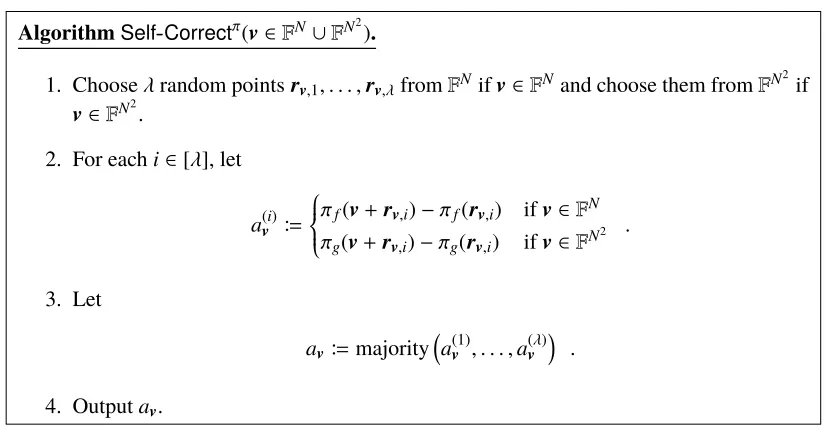
• Tensor-Product Test. LetSelf-Correctπbe the algorithm inFigure 2. Then, in Tensor-Product Test, choose two random points r1,r2∈FN, run

ar1 ←Self-Correct π_(r

1) , ar2 ←Self-Correct π₍_r

2) , and ar1⊗r2 ←Self-Correct π_(r

1⊗r2) ,

and check the following.

ar1ar2

?

=ar1⊗r2 .

• SAT Test. Choose a random pointσ = (σ1, . . . , σM) ∈ FM and define a quadratic function

Ψσ:FN →Fas

Ψσ(z)B

M

∑

i=1

σiΨi(z) .

Letψ_σ ∈FN _and_ψ′

σ ∈FN

2

be the coefficient vectors such that

Ψσ(z)=⟨ψσ,z⟩+⟨ψ′σ,z⊗z⟩ . (4.2)

Letc_σB∑_iM₌₁σici. Then, in SAT Test, run

a_ψ_σ ←Self-Correctπ(ψ_σ) and a_ψ′

σ ←Self-Correctπ(ψ′σ) ,

and check the following.

a_ψ_σ+a_ψ′

σ

?

=c_σ .

We remark that, formally,V = (V0,V1) is a pair of two algorithms as required byDefinition 1, whereV0(1λ,C)outputs a set of the queriesQfor the above tests along with its internal statestV, and V1(stV,x,y, π|Q) performs the above tests given the answersπ|Qfrom the PCP proof. The internal

statestV thatV0outputs is(σin,σout), where

σin B(σ1, . . . , σn)∈Fn and σout B(σM−m+1, . . . , σM)∈Fm ,

where it is assumed that the firstnequations inΨ(i.e., the equations{Ψi(z) = ci}i∈[n]) are those that

are associated with the input gates (i.e.,{zi = xi}i∈[n]) and the lastmequations inΨ(i.e.the equations

{ΨM−m+i(z)=cM−m+i}i∈[m]) are those that are associated with the output gates (i.e.,{zM−m+i =yi}i∈[n]).

Note thatV0(1λ,C) can indeed choose all the queries in parallel (without knowing the input x and

the outputy) since each of the queries is chosen independently of the results of the other queries and in addition the coefficient vectors of the equations of_Ψ(i.e.,_{_ψ_i,_ψ′_i_}i∈M) can be computed from the

circuitCin SAT Test. Also, note thatV1(stV,x,y, π|Q)can indeed perform the test (without knowing

the circuitC) sincec_σ =⟨σin,x⟩+⟨σout,y⟩can be computed fromstV in SAT Test.

Remark 4 (Query Complexity.). By inspection, one can see that that the query complexity of V is

κV(λ)Bλ(10λ+6). ^

(22)

AlgorithmSelf-Correctπ(v∈FN_∪_FN2_).

1. Chooseλrandom pointsrv,1, . . . ,rv,λfromFNifv∈FNand choose them fromFN 2

if

v∈FN2_.

2. For eachi∈[λ], let

a(i)_v B_πf(v+rv,i)−πf(rv,i) ifv∈F N

πg(v+rv,i)−πg(rv,i) ifv∈FN

2 .

3. Let

avBmajority (

a(1)v , . . . ,a(vλ) )

.

4. Outputav.

Figure 2: The self-correction algorithmSelf-Correct, which works given oracle access to_π₌(πf, πg)

4.3 Security Statement

FromSection 5toSection 9, we prove the following theorem, which states the no-signaling soundness of our PCP system.

Theorem 1(No-signaling Soundness of (P,V)). Let(P,V) be the PCP system in Sections 4.1 and

4.2, _{C_λ}_λ∈_N be any circuit family, and _κmaxbe any polynomial such that_κmax(λ) ≥ 2λ·max(8λ+ 3,m_λ)+κV(λ), wherem_λ is the output length ofC_λ andκV is the query complexity of(P,V). Then, for anyκmax-wise (computational) no-signaling cheating proverP∗, there exists a negligible function neglsuch that for every_λ_∈_N,

Pr

[

V1(stV,x,y, π∗)=1∧Cλ(x), y (Q,

stV)←V(1λ,C_λ) (x,y, π∗)←P∗(1λ,C_λ,Q)

]

≤negl(λ) .

Outline of the proof ofTheorem 1. InSection 5, we introduce a “relaxed verifier” such that if a cheating prover fools the original verifier with non-negligible probability, there exists another cheat-ing prover that fools the relaxed verifier with overwhelmcheat-ing probability. InSection 6, we show that if a cheating verifier convinces the relaxed verifier with overwhelming probability, we can obtain a “self-corrected PCP proof” from the cheating prover, where the self-corrected PCP proof satisfies several useful properties (namely, the ability to pass Linearity Test, Tensor-Product Test, and SAT Test on any points). InSection 7, we show that if a cheating verifier convinces the relaxed verifier with overwhelming probability, the self-corrected PCP proof matches the claimed computation, i.e., the assignment that we obtain from the self-corrected PCP proof on any small number of variables of

(23)

5 Analysis of Our PCP: Step 1 (Relaxed Verifier)

In this section, we introduce a “relaxed verifier”Vfor our PCP system. The relaxed verifier is designed so that if a no-signaling cheating prover can fool the original verifier with non-negligible probability, another no-signaling cheating prover can fool the relaxed verifier with overwhelming success proba-bility. In subsequent sections, we show the no-signaling soundness of our PCP system by showing that any no-signaling cheating prover cannot fool the relaxed verifier with overwhelming success proba-bility.

5.1 Construction

Recall that the original PCP verifierV, described inSection 4.2, makesλtrials of tests (where each trial consists of Linearity Test, Tensor-Product Test, and SAT Test) and accepts the proof if all the tests in all theλtrials succeed.

The relaxed verifierVmakesλtrials of tests in the same way as the original PCP verifier does, but accepts the proof even when tests in at most_µtrials fail (that is, accepts the proof if all the tests in at leastλ−µtrials succeed), whereµ = Θ(log2λ)is a parameter.13 We remark that, just like the original verifierV = (V0,V1), the relaxed verifierVis actually a pair of algorithms,(V0,V1), where

V0makes the queries andV1performs the tests. From the construction,V0is identical withV0.

5.2 Analysis

Lemma 1. Let_κmaxbe any polynomial such that_κmax(λ)≥2κV(λ), where_κV is the query complexity of(P,V). Then, for any circuit family{C_λ}_λ∈_N, if there exists aκmax-wise no-signaling proverP∗and a constantc>0such that

Pr

[

V1(stV,x,y, π∗)=1∧C_λ(x), y (Q,stV)←V0(1λ,Cλ) (x,y, π∗)←P∗(1λ,C_λ,Q)

]

≥λ−c _(5.1)

holds for infinitely many_λ_∈_N, there exists a(κmax−κV)-wise no-signaling prover_P∗and a negligible functionneglsuch that

Pr

[

V1(stV,x,y, π∗)=1∧Cλ(x), y

(Q,stV)←V0(1λ,Cλ) (x,y, π∗)←P∗(1λ,C_λ,Q)

]

≥1−negl(λ) (5.2)

holds for infinitely many_λ_∈_N.

We remark that Brakerski et al. [BHK17] prove essentially the same lemma asLemma 1(see Lemma 1 of the full version of their paper [BHK16]). Below, we give a proof ofLemma 1just for completeness. Since we only use the statement ofLemma 1in the subsequent sections, the readers who believe this lemma can skip the rest of this section.

Proof . Fix any polynomialκmaxsuch thatκmax(λ)≥2κV(λ), any circuit family{C_λ}_λ∈_N, anyκmax-wise no-signaling cheating proverP∗, and any constantc>0, and assume that Equation (5.1) holds.

The high-level idea of the relaxed cheating proverP∗is simple:P∗amplifies the success probability ofP∗by executing it repeatedly. That is, on input a set of queries Q, the relaxed cheating proverP∗

No-signaling Linear PCPs