Abstract
LU, KAIFENG. Estimation of Regression Coefficients in the Competing Risks Model with Missing Cause of Failure. (Under the direction of Dr. Anastasios A. Tsiatis.)
In many clinical studies, researchers are interested in the effects of a set of prognostic factors on the hazard of death from a specific disease even though patients may die from other competing causes. Often the time to relapse is right-censored for some individuals due to incomplete follow-up. In some circumstances, it may also be the case that patients are known to die but the cause of death is unavailable. When cause of failure is missing, excluding the missing observations from the analysis or treating them as censored may yield biased estimates and erroneous inferences. Under the assumption that cause of failure is missing at random, we propose three approaches to estimate the regression coefficients. The imputation approach is straightforward to implement and allows for the inclusion of auxiliary covariates, which are not of inherent interest for modeling the cause-specific haz-ard of interest but may be related to the missing data mechanism. The partial likelihood approach we propose is semiparametric efficient and allows for more general relationships between the two cause-specific hazards and more general missingness mechanism than the partial likelihood approach used by others. The inverse probability weighting approach is doubly robust and highly efficient and also allows for the incorporation of auxiliary covari-ates. Using martingale theory and semiparametric theory for missing data problems, the asymptotic properties of these estimators are developed and the semiparametric efficiency of relevant estimators is proved. Simulation studies are carried out to assess the perfor-mance of these estimators in finite samples. The approaches are also illustrated using the data from a clinical trial in elderly women with stage II breast cancer. The inverse proba-bility weighted doubly robust semiparametric estimator is recommended for its simplicity, flexibility, robustness and high efficiency.
Key words: Cause-specific hazard; Doubly robust; Imputation; Influence function;
ESTIMATION OF REGRESSION COEFFICIENTS IN THE COMPETING RISKS MODEL WITH MISSING CAUSE OF FAILURE
by
KAIFENG LU
A dissertation submitted to the Graduate Faculty of North Carolina State University
in partial fulfillment of the requirements for the Degree of
Doctor of Philosophy
STATISTICS
Raleigh March, 2002
APPROVED BY:
Anastasios A. Tsiatis Marie Davidian Chair of Advisory Committee
Biography
Acknowledgements
I would like to express my deepest gratitude and appreciation to my academic advisor, Dr. Anastasios A. Tsiatis, for his ceaseless inspiration and encouragement. Besides being one of leading researchers in the field of biostatistics, he is also one of the most respectable people one could ever associate with. Without his great guidance and patience, it would have been much more difficult for me to complete the doctorate degree.
I would also like to thank Dr. Sastry G. Pantula for his continuous support of my graduate study, Dr. David A. Dickey for his constant help on SAS, Dr. Marie Davidian for her useful tips on LATEX, Dr. John F. Monahan for his insightful explanation on simulation, Dr. Sujit Ghosh for his valuable comments on the draft. I am also grateful to Terry Byron for his aid on computing, Janice Gaddy for her assistance toward graduation. I would also like to especially thank my best friend, Pei-Yun Chen, for her relentless help in numerous aspects of my life. My thanks also go to other faculty, staff, and fellow students in our department. The congenial and conducive learning environment they provide has made my study such a pleasant and fruitful experience.
Contents
List of Tables vii
List of Abbreviations viii
1 Multiple Imputation Approach 1
1.1 Introduction . . . 1
1.2 Notation and Assumptions . . . 2
1.3 Imputation Procedure . . . 3
1.4 Asymptotic Properties . . . 5
1.5 Simulation Study . . . 6
1.6 Breast Cancer Example . . . 8
1.7 Discussion . . . 9
2 Efficient Partial Likelihood Approach 12 2.1 Introduction . . . 12
2.2 Notation and Assumptions . . . 13
2.3 Parameter Estimation . . . 14
2.4 Simulation Study . . . 16
2.5 Breast Cancer Example . . . 17
2.6 Discussion . . . 18
3 Inverse Probability Weighting Approach 20 3.1 Introduction . . . 20
3.2 Notation and Assumptions . . . 21
3.3 Full Data Influence Functions . . . 23
3.4 Observed Data Influence Functions . . . 25
3.5 Semiparametric Estimators . . . 26
3.6 Doubly Robust Semiparametric Estimators . . . 32
3.8 Simulation Study . . . 52
3.9 Breast Cancer Example . . . 54
3.10 Discussion . . . 55
4 Conclusions 58 4.1 Comparison . . . 58
4.2 Future Research . . . 59
Bibliography 61 Appendices 63 A Asymptotic Properties of Imputation Estimators . . . 64
B Semiparametric Efficiency of Partial Likelihood Estimator . . . 66
C Notion of Auxiliary Covariates . . . 67
List of Tables
1.1 Monte Carlo comparison of complete cases and imputation with sample size
of 200 . . . 10
1.2 Monte Carlo comparison of complete cases and imputation with sample size of 500 . . . 10
1.3 Robustness of imputation against misspecification of the % model . . . 11
1.4 Comparison of complete cases, Goetghebeur and Ryan, and imputation using the breast cancer data . . . 11
2.1 Monte Carlo comparison of complete cases, Goetghebeur and Ryan, and efficient likelihood approach with sample size of 200 . . . 19
2.2 Monte Carlo comparison of complete cases, Goetghebeur and Ryan, and efficient likelihood approach with sample size of 500 . . . 19
2.3 Comparison of complete cases, Goetghebeur and Ryan, and efficient likeli-hood approach using the breast cancer data . . . 19
3.1 Monte Carlo comparison of complete cases, imputation, and inverse proba-bility weighted estimators with sample size of 200 . . . 56
3.2 Monte Carlo comparison of complete cases, imputation, and inverse proba-bility weighted estimators with sample size of 500 . . . 57
3.3 Comparison of complete cases, Goetghebeur and Ryan, imputation, and dou-bly robust estimator using the breast cancer data . . . 57
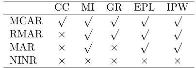
4.1 Inclusion of Auxiliary Covariates . . . 60
4.2 Missing Data Mechanism . . . 60
4.3 Robustness . . . 60
List of Abbreviations
CC complete case
CLT central limit theorem CP coverage probability
CPBT coverage probability via bootstrap DR doubly robust
EPL efficient partial likelihood ER estrogen receptor
GR Goetghebeur and Ryan IPW inverse probability weighted
IPWCC inverse probability weighted complete-case IPWDR inverse probability weighted doubly robust IPWLE inverse probability weighted locally efficient LHS left hand side
LIE law of iterated expectations MAR missing at random
MI multiple imputation
MLE maximum likelihood estimator
MPLE maximum partial likelihood estimator RHS right hand side
SE standard error
SEE standard error estimate
SEEBT standard error estimate via bootstrap SI single imputation
Chapter 1
Multiple Imputation Approach
1.1
Introduction
In many clinical studies where time to failure is of primary interest, patients may fail or die from one of many causes. For example, in a clinical trial that compares different therapies for breast cancer, interest may focus on death from breast cancer even though patients may die from other causes. A routine objective is to assess the effects of a set of prognostic covariates on the hazard rate of time to failure due to the cause of interest. In many studies, the cause of death information may be censored due to incomplete follow-up. In some circumstances, it may also be the case that patients are known to die but the cause of death is unavailable, e.g., whether death is attributable to the cause of interest or other causes may require documentation with information that is not collected or lost or cause may be difficult for investigators to determine for some patients (Andersen, Goetghebeur, and Ryan, 1996). If there were no missing cause of failure, the standard proportional hazards model can be used to model the cause-specific hazard of interest and the regression coefficients can be estimated using maximum partial likelihood estimators (Cox, 1972, 1975). However, when cause of failure is missing, excluding the missing observations from the analysis or treating them as censored may yield biased estimates and erroneous inferences. With missing cause of failure, Goetghebeur and Ryan (1995) proposed an approach by making assumptions directly on the relationship between the cause-specific hazard of interest and that of competing causes; these are assumed proportional, although this may be relaxed.
In Section 1.4, we state asymptotic properties of imputation estimators with proofs sketched out in the Appendix. In Section 1.5, we provide simulation results to show the relevance of the theory in finite samples. In Section 1.6, we illustrate the results using data from a clinical trial in stage II breast cancer. In Section 1.7, we give a brief discussion.
1.2
Notation and Assumptions
In this article, we will consider the situation where individuals may fail or die from one of two specific causes, one of which is of interest. The cause of interest will be referred to as cause 2 and all other causes of death will be combined and referred to as cause 1. If there was no censoring, the cause of death data could be summarized as (T∗,∆∗), whereT∗ denotes the time to death and ∆∗ denotes the cause of death, taking on values one or two. A set of covariates X is also defined with the primary goal of modeling the cause-specific hazard for the cause of interest to these covariates, namely
λ∗(t|x) = lim
h→0h −1P(t
≤T∗< t+h,∆∗ = 2|T∗ ≥t, X =x).
A popular model for this relationship is the proportional hazards model, which assumes that
λ∗(t|x) =λ(t)eβTx, (1.1) where β is the q-dimensional vector of regression coefficients and λ(t) is the unspecified baseline hazard for the cause of interest. For example, X may represent the indicator variable for treatment assignment and other baseline characteristics.
Because of incomplete follow-up, cause of death data are often censored by a variable
C, in which case the data we observe can be summarized by the variablesT = min(T∗, C) and ∆, which equals ∆∗ if T∗ ≤C and equals zero if T∗ > C, i.e., T is the time to failure or censoring and ∆ is the failure-censoring indicator taking on values zero, one, or two. To avoid nonidentifiability problems, we assume that C is conditionally independent of (T∗,∆∗) givenX, in which case the observable cause-specific hazards for causes 1 and 2, in the presence of censoring, defined as
λd(t|x) = lim h→0h
−1P(t≤T < t+h,∆ =d|T ≥t, X=x), d= 1,2,
are the same as the cause-specific hazards of interest. In particular,λ(t|x) =λ∗(t|x). With a sample of data (Ti,∆i, Xi), i = 1, . . . , n, the parameter β in the proportional hazards
model can be estimated using the maximum partial likelihood estimator after treating the values Ti observed for individuals whose ∆i is equal to zero or one as censored times.
otherwise. Assume that, if a subject is censored, this is known, so ∆i = 0 implies Ri = 1
and Ri = 0 implies ∆i = 1 or 2. Unlike previous methods, we may also define auxiliary
covariates Ai, which are not of inherent interest for modeling the cause-specific hazard
of interest but may be related to the missingness mechanism. For example, Ai may be
some post-treatment variable that may be related to the reason why the cause of death information was not collected but that would not be included in the model because it may affect the causal interpretation associated with the parameters for treatment effects. The observed data are thenOi = (Ri, Ti,∆i, Xi, Ai) ifRi= 1 andOi= (Ri, Ti, Xi, Ai) ifRi = 0,
independent acrossi.
The imputation procedure relies on the assumption of missing at random, or the prob-ability that cause of failure is missing given ∆i(>0) andWi = (Ti, Xi, Ai) depends only on
Wi, the information always observed on all subjects, and not on the unobserved ∆i,
P(Ri = 0|Wi,∆i >0,∆i) =P(Ri = 0|Wi,∆i >0).
This assumption stipulates thatRiand ∆iare independent given{Wi, I(∆i>0)}, expressed
equivalently as
P(∆i = 2|Wi,∆i >0, Ri = 0) = P(∆i = 2|Wi,∆i >0, Ri = 1)
= P(∆i = 2|Wi,∆i >0). (1.2)
The proposed imputation method exploits (1.2) as discussed in the next section.
Ordinarily, if no causes of failure are missing, auxiliary covariates are not used in es-timating β. When cause of failure is missing for some subjects, the assumption that it is missing at random depending only onI(∆i >0) and (Ti, Xi) may be untenable. However, it
may be possible to identify auxiliary covariates such that the missing at random assumption is plausible ifAiis included as above. The proposed approach allows information from such
Ai to be exploited to impute missing causes.
1.3
Imputation Procedure
As is customary, to form a completed data set, missingDi =I(∆i= 2) values are imputed
from the distribution ofDi conditional on the observed data. This distribution is Bernoulli
with success probability P(∆i = 2|Wi,∆i > 0, Ri = 0), which, by (1.2), equals P(∆i =
2|Wi,∆i >0) =%(Wi), say. We will assume that %(Wi) may be specified as a parametric
model in terms of a few unknown parametersγ and%(Wi) =%(Wi, γ0), whereγ0 is the true value of γ. A natural choice is the logistic regression model, logit %(Wi, γ) = WiTγ, but
of %(Wi), induced above, by choosing a suitable parametric model. For example, we might
include higher order polynomials and interaction terms for %(Wi, γ).
From (1.2), the success probability for the imputation, which equals%(Wi, γ0), is identi-cal toP(∆i = 2|Wi,∆i >0, Ri= 1). This suggests that%(Wi, γ0), and hence the imputation probability, may be deduced from the completed cases for whom (Ri = 1,∆i >0). In
par-ticular, under the parametric model%(Wi, γ), the maximum likelihood estimator ˆγofγ may
be obtained by fitting the model to the completed cases only, thus providing an estimate of
P(∆i= 2|Wi,∆i>0, Ri= 0).
For given γ, let Dij(Ri, γ) be the imputation of Di from the jth imputed data set. If
cause of failure is known (Ri= 1), we takeDij(Ri, γ) to beDi. If cause of failure is missing
(Ri = 0), we randomly choose Dij(Ri, γ) to be one or zero with probabilities%(Wi, γ) and
{1−%(Wi, γ)}, respectively.
The joint distribution of (Wi, Di) and {Wi, Dij(Ri, γ0)} may be seen to be the same. When Ri = 1, Dij(Ri, γ0) =Di, and when Ri = 0, {Wi, I(∆i >0)} arise from the
distri-bution of the observed data and Dij(Ri, γ0) from the conditional distribution of Di given
the observed data, so thatDij(Ri, γ0) is a draw from the joint distribution of the full data. Therefore, if true parameters and a parametric model for% were known, then a single im-putation of any missing data is as good as if you could conduct the experiment with no missingness.
Since ˆγ is the maximum likelihood estimator for γ, then for a correctly specified model
%(Wi, γ), it is consistent and we can treat it as if it were the true parameter. Because we can
now generate data that are asymptotically as good as the original experiment, we can fit the proportional hazards model to a completed data set. We can carry out the imputation procedure multiple times and average the maximum partial likelihood estimators. The resulting estimator is the multiple imputation estimator we propose. Because each estimate is consistent, their average is also.
Although Rubin (1987) suggests a method for estimating the variance of the average of quantities from m imputed data sets, it is not appropriate here; because we generate imputations from the conditional distribution of missing data given the observed evaluated at ˆγ, where ˆγis held fixed acrossj, our imputation is not proper in the sense of Rubin (1987). Results of Wang and Robins (1998) indicate that under these conditions, which they refer to as type B multiple imputation, Rubin’s variance expression will yield an inconsistent estimator for the true sampling variance. Consequently, we derive a variance estimator directly which accounts for all sources of variability, including the variability in ˆγ.
We would like to make a few remarks regarding the probability model %(Wi, γ). It is
hazards for the two failure types, conditional on (X, A) and with w= (t, x, a), by
λ(t|x, a)
λ1(t|x, a) =
%(w)
1−%(w)
. (1.3)
This implies that the functional relationship of %(Wi) to Wi is induced from the ratio of
cause-specific hazards. Note that the cause-specific hazards in (1.3) are conditional on both the covariates of interest X and the auxiliary covariatesA and may not necessarily be the same as the cause-specific hazard of interest given in (1.1), which only conditions on X. For convenience, we have used a parametric model to model a relationship which is of no inherent interest to us and one which would be left arbitrary if there were no missing cause of death information. Therefore, as pointed out by Satten, Datta, and Williamson (1998), it will be important to examine the robustness of our estimator to misspecification of this probability model. This issue, although difficult to establish theoretical properties for, will be considered empirically in Section 5.
1.4
Asymptotic Properties
In establishing the consistency and asymptotic normality of imputation estimators, we assume that both the proportional hazards model (1.1) and the model for the probability that a missing cause is that of interest%(Wi, γ) are correctly specified. The results are listed
below while the proofs are outlined in Appendix A. Let
µX(t) =
E{Xeβ0TXI(T ≥t)}
E{eβT
0XI(T ≥t)}
.
Also denote %γ(W) as the derivative of %(W, γ) with respect toγ evaluated atγ0, and
Iγ=E
{%γ(W)}⊗2
P(R= 1,∆>0|W)
%(W){1−%(W)}
.
Proposition 1 Each single imputation estimator, βˆj(j = 1, . . . , m), is consistent and
n1/2( ˆβj−β0)is asymptotically normal with asymptotic variance equal toVS−1VSIVS−1, where
VSI = VS+E[{X−µX(T)}P(∆>0|W)%Tγ(W)]Iγ−1
E[%γ(W)P(∆>0|W){X−µX(T)}T]
−E[{X−µX(T)}P(R = 1,∆>0|W)%Tγ(W)]Iγ−1
E[%γ(W)P(R= 1,∆>0|W){X−µX(T)}T],
and VS = RE[{X−µX(t)}⊗2eβ
T
0XI(T ≥t)]λ(t)dt is the asymptotic variance of the score
The variability of ˆγ plays a role in both the second term and the third term, while the missingness contributes to their nonnegative difference. Without missing cause of failure, the second term and the third term are identical and would vanish, leavingVSI =VS, which
leads to the familiar asymptotic results for partial likelihood estimators for the proportional hazards model.
Proposition 2 The multiple imputation estimator, βˆ, is consistent and n1/2( ˆβ −β0) is asymptotically normal with asymptotic variance equal to VS−1VM IVS−1, where
VM I = VSI−(1−m−1)E[{X−µX(T)}⊗2P(R = 0|W)%(W){1−%(W)}].
It is evident that the second term, which measures the reduction in variability of the multiple imputation estimator over the single imputation estimator, is introduced through imputing the missing data multiple times. The more imputation we use, the greater the reduction in the asymptotic variance. The relative magnitude of VSI and the second term
will determine the number of imputations we might use.
Note that the estimate of the asymptotic variance can be obtained easily by manipulating readily available statistical software output. For example, ˆIγ can be obtained by inverting
the variance estimate of ˆγand dividing it byn; ˆVScan be obtained by inverting the variance
estimates from themimputed data sets, dividing them byn, and averaging them across the
m imputations; and all other quantities can be consistently estimated using their sample analogs.
1.5
Simulation Study
Several simulations were carried out to evaluate the performance of imputation estimators. We considered the case where the treatment indicator Xi is the only prognostic covariate
with P(Xi = 1) = P(Xi = 0) = 1/2, and we also considered a single auxiliary covariate
Ai, drawn from the standard normal distribution, independently of Xi. For each subject
i, we took Ti = min(T2i, T1i, Ci), where T2i, T1i, and Ci were generated independently,
conditional on (Xi, Ai), as described below; the resulting hazards forT2,T1, andCwere thus the same as the cause-specific hazards λj(t|x, a) for j = 2,1,0, respectively. Conditional
on (Xi = x, Ai = a), T2i was generated from the exponential distribution with hazard
function λ(t|x, a) = λ(t|x) = φeβx, where φ = 1, β = −0.2. Let logit%(W
i, γ) = γ1 +
γ2Ti+γ3Xi+γ4Ai, where γ = (1,−0.2,0.5,2). Then by (1.3), T1i follows the Gompertz
may not necessarily equal λ(t|x, a). The censoring time Ci was generated from the
right-truncated exponential distribution with hazard rate λC = 0.01 and truncating time L= 5,
independently of all other random variables. With such a choice of parameter values, we will have, on average, 55% failures from the cause of interest, 30% failures from other causes, and 15% censored observations. The missing data mechanism was determined by logitP(Ri = 0|∆i > 0, Wi, ψ) = ψ1 +ψ2Ti +ψ3Xi +ψ4Ai, with different choices of ψ
corresponding to different scenarios of missingness.
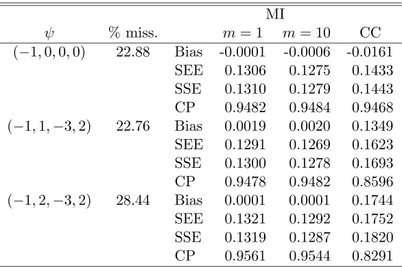
For sample sizesn= 200,500, we carried out 10,000 simulations to compare the multiple imputation methods with m = 1 and m = 10 imputation and the complete case analysis. The results are summarized in Tables 1.1 and 1.2, where SEE denotes the empirical Monte Carlo average of our standard error estimates, SSE denotes the Monte Carlo standard error of the parameter estimates, and CP denotes the empirical coverage probability of the 95% confidence interval defined as ˆβ±1.96SE( ˆβ).
The scenario where ψ= (−1,0,0,0) corresponds to the case where the cause of death is missing completely at random. For this scenario, all analyses gave similar results, although the imputation methods were more efficient. When ψ = (−1,1,−3,2), approximately the same proportion of missing observations were produced, but now the complete case analy-sis yielded large bias and poor coverage which becomes worse as the sample size increases. Whenψ= (−1,2,−3,2), the proportion of missing observations increased from 23% to 28% and the complete case analysis performed more poorly since it produced even larger biases and lower coverage probabilities. In all cases, imputation estimators were asymptotically unbiased, had the smallest standard errors, and achieved the nominal 95% coverage prob-ability, with multiple imputation performing slightly better than single imputation. Also, the average of standard errors was very close to the Monte Carlo standard error, justifying our estimator of the asymptotic variance.
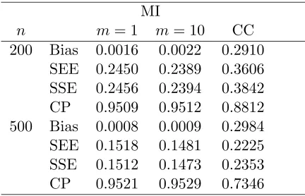
As pointed out in Satten et al. (1998), it is important to study robustness of parameter estimates from a semi- or non-parametric procedure when it uses data that were imputed using a parametric model. To investigate the robustness of the imputation procedure against misspecification of the parametric model for%, we generated the survival times, T1i, due to
the competing causes, from gamma, log normal, log logistic as well as Weibull distributions. None of these distributions will induce a simple linear logistic regression model for %. We report on the case where we generatedT1i from a Weibull distribution with shape parameter
0.5 and scale parameter exp[2{log(0.5)−log(φ) +γ1+γ2+ (γ3−β)X+γ4A}]. In this case, the true model for% is logit%(Wi) =γ1+γ2−(a−1) logTi+γ3Xi+γ4Ai, yet we imputed
missing cause of death fitting a simple linear logistic model. The results are included in Table 1.3, where we considered the missingness scenarioψ= (−1,2,−3,2) for sample sizes
resulting from the use of the misspecified model. Although, not presented here, for all other distributions considered for T1i mentioned above, the estimates for β never showed any
appreciable bias and achieved the nominal coverage probability.
1.6
Breast Cancer Example
1.7
Discussion
Table 1.1: Monte Carlo comparison of complete cases and imputation with sample size of 200
MI
ψ % miss. m= 1 m= 10 CC
(−1,0,0,0) 22.86 Bias -0.0026 -0.0020 -0.0174 SEE 0.2084 0.2037 0.2295 SSE 0.2080 0.2040 0.2301 CP 0.9517 0.9519 0.9501 (−1,1,−3,2) 22.84 Bias -0.0007 -0.0009 0.1257 SEE 0.2066 0.2029 0.2603 SSE 0.2087 0.2056 0.2690 CP 0.9511 0.9504 0.9231 (−1,2,−3,2) 28.53 Bias 0.0028 0.0021 0.1662 SEE 0.2116 0.2070 0.2812 SSE 0.2144 0.2096 0.2944 CP 0.9516 0.9493 0.9104
Table 1.2: Monte Carlo comparison of complete cases and imputation with sample size of 500
MI
ψ % miss. m= 1 m= 10 CC
Table 1.3: Robustness of imputation against misspecification of the % model MI
n m= 1 m= 10 CC 200 Bias 0.0016 0.0022 0.2910
SEE 0.2450 0.2389 0.3606 SSE 0.2456 0.2394 0.3842 CP 0.9509 0.9512 0.8812 500 Bias 0.0008 0.0009 0.2984 SEE 0.1518 0.1481 0.2225 SSE 0.1512 0.1473 0.2353 CP 0.9521 0.9529 0.7346
Table 1.4: Comparison of complete cases, Goetghebeur and Ryan, and imputation using the breast cancer data
CC GR MIa
4+ nodes 0.71[0.3065] 0.57[0.2803] 0.60[0.2618] ER-neg. 1.70[0.4861] 1.59[0.4822] 1.61[0.4794]
a
Chapter 2
Efficient Partial Likelihood
Approach
2.1
Introduction
We extend their ideas to the more general settings where the probability of having a missing cause of death may depend on the covariates as well as time and where the ratio of the two baseline cause-specific hazards may also depend on time. This is achieved through the construction of an estimator using the full partial likelihood above. We show that the resulting estimator is consistent, asymptotically normal, and semiparametric efficient, under the more general missingness assumptions.
We introduce our notation and assumptions in Section 2.2. In Section 2.3, we propose the estimator which arises as the solution to the estimating equation based on the informative partial likelihood. Consistency and asymptotic normality of the resulting estimator will then follow from the martingale theory. Semiparametric efficiency can be established using semiparametric theory. Simulation results are also presented to compare the performance of our estimator with that of the complete-case estimator and that of the Goetghebeur and Ryan estimator. We conclude with an application followed by a brief discussion.
2.2
Notation and Assumptions
In this article, we consider a sample ofnindependent individuals, each of whom can die of fail from one of two possible causes which we refer to as causes two and one, respectively, or can be subject to a noninformative censoring mechanism. Typically, the data for individual
iare{Ti,∆i, Xi}, whereTiis the time to failure or censoring; ∆iis an indicator taking values
zero, one, or two, as theith individual was censored, died from cause one, or died from cause two, respectively; Xi denotes a vector of covariates. Let λδ(t|x), δ = 2,1,0 be the
cause-specific hazards for failure from cause two, failure from cause one, or censoring, respectively. Suppose that the cause-specific hazards for causes two and one follow proportional hazards relationships, namely,
λδ(t|x) =λ(t)rδ(t, x, β), δ= 1,2, (2.1)
whereβis an unknownq-dimensional vector of parameters andλ(t) is the common unspec-ified baseline cause-specific hazard. No assumptions are made on the cause-specific hazard of censoring,λ0(t|x), or the marginal distribution ofX,pX(x).
that all information about time that is common to the two cause-specific hazards has been incorporated into the common baseline cause-specific hazard.
Also note that we could have formulated the model with separate regression parameter vectors {β1, β2} for the two failure causes. There may be examples, however, where some parameters are common to the two failure causes. Therefore, it is convenient to formulate the model with one vector of parameters β which contains all the different parameters in
{β1, β2} (c.f., Andersen, Borgan, Gill, and Keiding, 1997, p. 478).
In some circumstances, cause of failure might be missing for some individuals, in which case, we use Ri as the missingness indicator, taking values one or zero as the cause of
failure ∆i(> 0) is observed or missing. We assume that cause of failure is missing at
random (Rubin, 1976), in the sense that the probability of having a missing cause of failure does not depend on the latent cause of failure, i.e.,
P(Ri = 1|Zi,∆i >0) = π(Ti, Xi), (2.2)
where π is an unknown function of time and covariates, taking values in the unit interval. Note that we allow the missingness probability to depend on both time and covariates, whereas Goetghebeur and Ryan (1995) allows the missingness probability to depend on time only. In the presence of missing cause of failure, the observed data for the ith individual can be summarized asOi ={Ri, Ti, I(∆i = 0), RiI(∆i= 1), RiI(∆i = 2), Xi}.
2.3
Parameter Estimation
For an uncensored individual, one of the following three types of events can occur at the time of failure, i.e., failure from cause one, failure from cause two, or failure with unknown cause. Let Ni(t) = {Ni1(t), Ni2(t), Niu(t)} be a multivariate counting process indicating
the failure type. Based on the assumptions (2.1) and (2.2), the corresponding intensity processes are given by
λ∗i1(t, Xi) = Yi(t)π(t, Xi)r1(t, Xi, β0)λ(t),
λ∗i2(t, Xi) = Yi(t)π(t, Xi)r2(t, Xi, β0)λ(t),
λ∗iu(t, Xi) = Yi(t){1−π(t, Xi)}r.(t, Xi, β0)λ(t),
respectively, where Yi(t) = I(Ti ≥ t) denotes whether individual i is at risk at time t,
r.(t, x, β) =r1(t, x, β) +r2(t, x, β), andβ0 denotes the true value of β.
event occurs, but without conditioning on the type of event, i.e.,
L(β) = Y
t≥0
n
Y
i=1
"
r1(t, Xi, β)
Pn
j=1r.(t, Xj, β)Yj(t)
#dNi1(t)
×
"
r2(t, Xi, β)
Pn
j=1r.(t, Xj, β)Yj(t)
#dNi2(t)
×
"
r.(t, Xi, β)
Pn
j=1r.(t, Xj, β)Yj(t)
#dNiu(t)
,
whereQ
t≥0 denotes product-integration (c.f., Gill and Johansen, 1990).
Let{rd0(t, Xi, β), r00d(t, Xi, β)}denote the first two partial derivatives of rd(t, Xi, β) with
respect toβ ford= 1,2, and let
m(t, β) =
Pn
j=1r0.(t, Xj, β)Yj(t)
Pn
j=1r.(t, Xj, β)Yj(t)
,
v(t, β) =
Pn
j=1r.00(t, Xj, β)Yj(t)
Pn
j=1r.(t, Xj, β)Yj(t)
,
then the corresponding score equation is U(β) = 0, where
U(β) =
n
X
i=1
Z r0
1(t, Xi, β)
r1(t, Xi, β)
dNi1(t)
+
Z r0
2(t, Xi, β)
r2(t, Xi, β)
dNi2(t)
+
Z r0
.(t, Xi, β)
r.(t, Xi, β)
dNiu(t)
−
Z
m(t, β)dNi.(t)
,
and the observed information is
I(β) = −
n
X
i=1
( Z "r00
1(t, Xi, β)
r1(t, Xi, β) −
r0
1(t, Xi, β)
r1(t, Xi, β)
⊗2#
dNi1(t)
+
Z "r00
2(t, Xi, β)
r2(t, Xi, β) −
r0
2(t, Xi, β)
r2(t, Xi, β)
⊗2#
dNi2(t)
+
Z "r00
.(t, Xi, β)
r.(t, Xi, β) −
r0
.(t, Xi, β)
r.(t, Xi, β)
⊗2#
dNiu(t)
−
Z h
v(t, β)− {m(t, β)}⊗2idNi.(t)
o
,
Note that U(β0) is a martingale and hence the score equation can be used to obtain a consistent estimator of β, say ˆβn. In addition, it is straightforward to show that, when
evaluated at the truth, the observed information matrixI(β0) =−∂U(β)/∂β|β=β0 has the
same expectation as the covariation process of the score vector U(β0). Consistency and asymptotic normality of ˆβn follow from arguments similar to those used by Andersen and
Gill (1982) and the asymptotic variance can be consistently estimated by n−1{I( ˆβn)}−1.
Using semiparametric theory (e.g., Newey, 1990; Bickel, Klaasen, Ritov, and Wellner, 1993; Robins, Rotnitzky, and Zhao, 1994), we show that the influence function of our proposed estimator is the efficient influence function. The proof is outlined in Appendix B.
2.4
Simulation Study
Several simulations were carried out to evaluate the performance of different estimators. We considered the situation where the treatment assignmentXi was the only covariate and
Xi ∼ Bernoulli(0.5). For each subject i, we took Ti = min(T2i, T1i, Ci), where T2i, T1i,
and Ci were generated independently, conditional onXi, as described below; the resulting
hazards for T2, T1, and C0 were thus the same as the cause-specific hazards λδ(t|x) for
δ = 2,1,0, respectively. Conditional on Xi = x, T2i was generated from an exponential
distribution with constant hazardλ2(t|x) =φeβx, where φ= 0.8 andβ = 0.5. Comparison of different approaches was based on the estimation of β. In addition, T1i was generated
from a Gompertz distribution with hazard function λ1(t|x) =eγ1t+γ2x. Consequently, the ratio between the two baseline cause-specific hazards wasλ2(t)/λ1(t) =φexp(−γ1t), which is not constant over time unlessγ1 = 0. However, as pointed out by Goetghebeur and Ryan (1995), the efficient partial likelihood estimator is more sensitive than the Goetghebeur and Ryan partial likelihood estimator to violations of the proportionality assumption relating the two baseline cause-specific hazards. Therefore, we only need to consider the case when
γ1 = 0. Furthermore, the censoring timeCi was generated from an exponential distribution
with constant hazardλC = 0.4. Finally, the missingness indicatorRi was generated from a
Bernoulli distribution with success probability depending only on (Ti, Xi) to comply with
the MAR assumption. In particular, we let logit π(Ti, Xi) =ψ0+ψ1Ti+ψ2Xi, with different
values ofψ corresponding to different scenarios of missingness.
For sample sizes n = 200,500, we carried out 1000 simulations to compare different approaches. With such parameter values, we will have, on average, 34% to 46% failures from cause two (∆i = 2), 36% to 52% failures from cause one (∆i = 1), and 14% to 18%
censored observations (∆i = 0). For all cases of missing data mechanism we considered, the
proportion of missing observations (Ri = 0) ranged between 17% and 29%. The results of
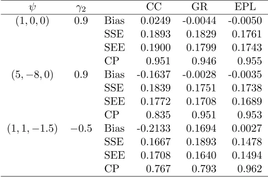
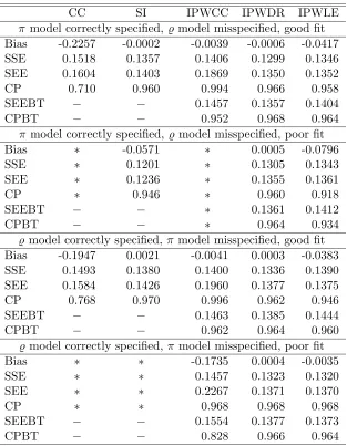
partial likelihood approach (GR), and the efficient partial likelihood approach (EPL) are summarized in terms of the sampling bias, the sampling standard error (SSE), the sampling average of the standard error estimates (SEE), and the empirical coverage probability (CP) of the asymptotic 95% confidence interval in Tables 2.1 and 2.2.
The scenario where ψ= (1,0,0) corresponds to the case where cause of failure is miss-ing completely at random. For this scenario, all analyses give similar results although our estimates are the most efficient. Whenψ= (5,−8,0), which corresponds to the case where the probability of having a missing cause of failure depends on time only, the naive com-plete case estimator is biased and has a coverage probability substantially lower than the nominal level, but the Goetghebeur and Ryan estimator still performs well because their missingness assumption is still met. For ψ= (1,1,−1.5), in which case, the probability of having a missing cause of failure depends on both time and covariate, the naive complete case estimator is again biased as expected, so is the Goetghebeur and Ryan estimator. Fur-thermore, the Goetghebeur and Ryan variance estimator underestimates the true sampling variation, resulting in a further reduced coverage probability. In all cases, our efficient likelihood approach performs well.
2.5
Breast Cancer Example
2.6
Discussion
Table 2.1: Monte Carlo comparison of complete cases, Goetghebeur and Ryan, and efficient likelihood approach with sample size of 200
ψ γ2 CC GR EPL
(1,0,0) 0.9 Bias 0.0162 -0.0123 -0.0157 SSE 0.3163 0.2986 0.2873 SEE 0.3055 0.2888 0.2792 CP 0.939 0.940 0.941 (5,−8,0) 0.9 Bias -0.1666 -0.0094 -0.0115 SSE 0.2842 0.2819 0.2786 SEE 0.2839 0.2733 0.2701 CP 0.904 0.946 0.947 (1,1,−1.5) −0.5 Bias -0.2115 0.1793 0.0097 SSE 0.2707 0.3070 0.2378 SEE 0.2738 0.2656 0.2381 CP 0.880 0.891 0.956
Table 2.2: Monte Carlo comparison of complete cases, Goetghebeur and Ryan, and efficient likelihood approach with sample size of 500
ψ γ2 CC GR EPL
(1,0,0) 0.9 Bias 0.0249 -0.0044 -0.0050 SSE 0.1893 0.1829 0.1761 SEE 0.1900 0.1799 0.1743 CP 0.951 0.946 0.955 (5,−8,0) 0.9 Bias -0.1637 -0.0028 -0.0035 SSE 0.1839 0.1751 0.1738 SEE 0.1772 0.1708 0.1689 CP 0.835 0.951 0.953 (1,1,−1.5) −0.5 Bias -0.2133 0.1694 0.0027 SSE 0.1667 0.1893 0.1478 SEE 0.1708 0.1640 0.1494 CP 0.767 0.793 0.962
Table 2.3: Comparison of complete cases, Goetghebeur and Ryan, and efficient likelihood approach using the breast cancer data
CC GR EPL
Chapter 3
Inverse Probability Weighting
Approach
3.1
Introduction
In some circumstances, it may also be the case that auxiliary covariates ,which are not of inherent interest for modeling the cause-specific hazard of interest, but which may be related to the missingness mechanism, are available. For example, we may be able to identify some post-treatment variable which is related to the reason why the cause of death information was not collected, but we would not include it in the proportional hazards model because it may affect the causal interpretation associated with the parameters for treatment effects. When the auxiliary covariates are included in the model of missingness mechanism, it might be reasonable to assume that cause of failure is missing at random, whereas the MAR assumption might not hold if the auxiliary covariates are not included.
In this article, we take a different approach by using two parametric models to model the missingness probability and the probability that a missing cause is the cause of interest, respectively, while allowing the inclusion of additional auxiliary covariates. Using semi-parametric theory (e.g., Newey, 1990; Bickel, Klaasen, Ritov, and Wellner, 1993; Robins, Rotnitzky, and Zhao, 1994), we identify various classes of inverse probability weighted (IPW) semiparametric estimators. In Section 3.3, we obtain the space of all full data in-fluence functions and the full data efficient score. In Section 3.4, we derive the space of all observed data influence functions. In Section 3.5, we introduce a class of estimating equations whose solutions correspond to all semiparametric estimators when the missing-ness mechanism is not known but can be correctly specified through a parametric model. In Section 3.6, we construct a class of estimating equations whose solutions define all doubly robust semiparametric estimators when either of the two parametric models is correctly specified. In Section 3.7, we identify the observed data efficient score and construct an esti-mating equation based on the observed data efficient score. The solution to the estiesti-mating equation is the locally semiparametric efficient estimator, which will be fully efficient if all parametric models are correctly specified. Simulation results are then presented to compare three IPW semiparametric estimators with the complete case estimator and the imputation estimator, followed by a revisit of the breast cancer example using the doubly robust IPW semiparametric estimator. A brief discussion is also provided to conclude this article.
3.2
Notation and Assumptions
asymptotically linear with influence function ϕif
n1/2( ˆβn−β0) =n−1/2
n
X
i=1
ϕi+op(1).
Consider the generic semiparametric model indexed by some finite, say q-dimensional pa-rameter of interestβ and the infinite dimensional nuisance parameter η. The Hilbert space
Hconsists of allq×1 random vectors of mean zero and square integrable measurable func-tions ofZ equipped with covariance inner product. The nuisance tangent space Λ is defined to be the mean square closure of the set of all random vectorsBSγ, whereSγ is the score for
γ in some regular parametric submodel andBis a conformable constant matrix withqrows. Also, Π[h|Λ] denotes the projection of any vectorh∈ Hon a closed linear space such as Λ. The semiparametric variance bound equals the inverse of the variance of Seff = Π[Sβ|Λ⊥],
where Sβ is the score for β and Seff is called the efficient score. In addition, we will use
the superscript “F” to distinguish the full data model from the observed data model. For example, we let SβF, ΛF,SeffF , and ΛF∗⊥ be the full data score for β, the full data nuisance
tangent space, the full data efficient score, and the space of full data influence functions, respectively.
The complete data for a single observation can be represented as Z = (T,∆, X, A), where T is the observed time to failure or censoring, ∆ is an indicator taking values two, one or zero as the individual failed from cause two, failed from cause one, or was censored, respectively. Without loss of generality, assume cause two is the cause of interest and cause one is the competing cause. In addition,Xdenotes the vector of covariates of interest, which is assumed to be related to the cause-specific hazard of interest through the proportional hazards model,
λ(t|X) =λ(t)eβTX, (3.1) where β is the q-dimensional vector of regression coefficients and λ(t) is the unspecified baseline cause-specific hazard. Also, A denotes auxiliary covariates which are not of in-herent interest for modeling the cause-specific of interest but which may be related to the missingness mechanism.
In certain instances, patients are known to die but the cause of death information is not available, in which case, we useRas the complete case indicator taking values one or zero as the cause of death is known or missing, so that the observed data for a typical observation can be summarized as O ={R, GR(Z)}={R, T, X, A, I(∆ = 0), RI(∆ = 1), RI(∆ = 2)}.
Write W = (T, X, A), then G1(Z) = Z = (W,∆). Also let Q = {W, I(∆ > 0)}, which denotes variables that are always observed, thenG0(Z) =Q. Furthermore, assume that
then {R⊥⊥∆|Q}, so that (3.2) implies that cause of failure is missing at random (Rubin, 1976). Writeπ(W) =P(R= 1|W,∆>0) and assume π(W) > >0 with probability one so that the probability of observing complete data is bounded away from zero.
3.3
Full Data Influence Functions
In the absence of missing data, the density for a typical observation can be factorized as
P(T =t,∆ =δ, X =x, A=a) = pA|T,∆,X(a|t, δ, x)
×exp[−{Λ(t|x) + Λ1(t|x) + Λ0(t|x)}]
×λ(t|x)I(δ=2)λ1(t|x)I(δ=1)λ0(t|x)I(δ=0)
×pX(x),
where pA|T,∆,X is the conditional density of A given (T,∆, X), {λ1(t|x), λ0(t|x)} are the conditional cause-specific hazard for failure from the competing cause and the conditional cause-specific hazard for censoring, givenX=x, respectively,{Λ(t|x), Λ1(t|x), Λ0(t|x)}are the corresponding cumulative cause-specific hazards, andpX is the marginal density of X.
Therefore, the log-likelihood for a typical observation can be written as
`F(Z) = −Λ(T|X) +I(∆ = 2) logλ(T|X)
−Λ1(T|X) +I(∆ = 1) logλ1(T|X)
−Λ0(T|X) +I(∆ = 0) logλ0(T|X) + logpX(X)
+ logpA|T,∆,X(A|T,∆, X). (3.3) Write Λ(t) =Rt
0λ(s)ds, then, under assumption (3.1), (3.3) reduces to
`F(β, Z) = −Λ(T)eβTX+I(∆ = 2){logλ(T) +βTX}
−Λ1(T|X) +I(∆ = 1) logλ1(T|X)
−Λ0(T|X) +I(∆ = 0) logλ0(T|X) + logpX(X)
+ logpA|T,∆,X(A|T,∆, X). (3.4)
Since the nuisance parameters{λ(t), λ1(t|x), λ0(t|x), pX(x), pA|T,∆,X(a|t, δ, x)}are
func-tionally independent and separate from each other in the log-likelihood (3.4), the full data nuisance tangent space can be written as a direct sum of five orthogonal spaces,
where Λ1s is associated with λ(t), Λ2s is associated with λ1(t|x), Λ3s is associated with
λ0(t|x), Λ4s is associated withpX, and Λ5s is associated withpA|T,∆,X, respectively.
It is straightforward to show that Λ1s =
Z
α(t)dM(t) :∀αq×1(t)
,
wheredM(t) =dN(t)−λ(t)eβT
0XI(T ≥t)dt, N(t) =I(T ≤t,∆ = 2).
On the other hand, had no restrictions been put on the form of the cause-specific hazard of interest, the log-likelihood (3.3) would correspond to a saturated model, so that the entire full data Hilbert space can be written as the direct sum of five orthogonal spaces,
HF = Λ∗1s+ Λ2s+· · ·+ Λ5s,
where Λ∗1s is associated with λ(t|x). It is straightforward to show that
Λ∗1s=
Z
a(t, X)dM(t) :∀aq×1(t, X)
.
Therefore, the space orthogonal to the full data nuisance tangent space, i.e. ΛF⊥, is the subspace of Λ∗1s that is orthogonal to Λ1s. By the projection theorem, it is straightforward
to show that
ΛF⊥=
Z
{a(t, X)−µa(t)}dM(t) :∀aq×1(t, X)
, (3.5)
where
µa(t) =
E{a(t, X)eβ0TXI(T ≥t)}
E{eβT
0XI(T ≥t)}
.
For an element of ΛF⊥, say ϕF(Z), to be an influence function for a semiparametric
estimator for β, we must also have E{ϕF(Z)SβF T(Z)} = Iq, where SβF(Z) is the full data
score forβ andIq is the q×q identity matrix.
From (3.4),
SβF(Z) =
Z
XdM(t). (3.6)
By standard properties for martingales (e.g., Fleming and Harrington, 1991),
E
Z
{a(t, X)−µa(t)}dM(t)SβF(Z)
=
Z
E[{a(t, X)−µa(t)}{X−µX(t)}Teβ
T
0XI(T ≥t)]λ(t)dt
≡ V(a, X),
where “≡” means “denoted as” and
µX(t) =
E{XeβT
0XI(T ≥t)}
E{eβTX
Therefore, the space of full data influence functions is given by
ΛF∗⊥=
V−1(a, X)
Z
{a(t, X)−µa(t)}dM(t) :∀aq×1(t, X)
. (3.7)
In addition, by (3.5) and (3.6), the full data efficient score is given by
SeffF (Z) =
Z
{X−µX(t)}dM(t). (3.8)
3.4
Observed Data Influence Functions
First suppose that π(W) is completely known as in a designed study, then
P(R= 1|Z) =π(W)I(∆>0) +I(∆ = 0)≡π(Q).
By Proposition 8.1 of Robins et al. (1994), the space of all observed data influence functions is given by
Λ⊥0∗ =
R π(Q)Λ
F⊥
∗ + Λ2, (3.9)
where Λ2={L2(O)∈ H:E{L2(O)|Z}= 0}. Write
L2(O) =RL21(Z) + (1−R)L20(Q), (3.10) then
E{L2(O)|Z}=π(Q)L21(Z) +{1−π(Q)}L20(Q).
Set E{L2(O)|Z)} = 0, we have L21(Z) =−{1−ππ(Q(Q))}L20(Q). Substituting it into (3.10), a typical element of Λ2 is given by
L2(O) =−{
R−π(Q)}
π(Q) L20(Q), (3.11) whereL20(Q) is an arbitrary q×1 function ofQsatisfying E{LT20(Q)L20(Q)}<∞.
By (3.7), (3.9), and (3.11), a typical element of Λ⊥
0∗ is given by
ϕ0(O) = R
π(Q)V
−1(a, X)Z
{a(t, X)−µa(t)}dM(t)
−{Rπ−(πQ()Q)}L20(Q).
Now suppose that the missingness mechanism π(W) is not known but we can correctly specify a parametric model, say π(W) =π(W, ψ), then
By Proposition 8.1 of Robins et al. (1994), the space of all observed data influence functions is given by
Λ⊥∗ = Λ⊥0∗−Π[Λ⊥0∗|Λψ],
where Λψ is the nuisance tangent space for ψ. Therefore, a typical element of Λ⊥∗ is given
by
ϕ(O) =ϕ0(O)−Π[ϕ0(O)|Λψ].
Note that the observed data likelihood for ψis
n
Y
i=1
{π(Qi, ψ)}Ri{1−π(Qi, ψ)}1−Ri.
Hence, the log-likelihood forψ for a typical observation is
`(ψ, O) =Rlogπ(Q, ψ) + (1−R) log{1−π(Q, ψ)}.
Consequently, the score vector for ψis
Sψ(O) = {
R−π(Q)}πψ(Q)
π(Q){1−π(Q)} , (3.12) where πψ(Q) denotes the partial derivative of π(Q, ψ) with respect to ψ and evaluated at
ψ=ψ0. A typical element of Λψ is given byBSψ for some arbitrary conformable matrixB
withq rows. By (3.12) and (3.11), Λψ ⊂Λ2.
3.5
Semiparametric Estimators
Assume that the parametric model for the missingness mechanism, π(W) = π(W, ψ), is correctly specified. Let ˆψnbe the MLE ofψ, andψ0 be the true value of ψ, then ˆψn→p ψ0.
It is shown in Section 3.4 that a typical element of Λ⊥0∗ is given by
ϕ0(O) =V−1(a, X)ϕ∗0(O), where
ϕ∗0(O) = R
π(Q, ψ0)
Z
{a(t, X)−µa(t)}dM(t)
−{R−π(Q, ψ0)}
π(Q, ψ0) L(Q)
= R
π(Q, ψ0)
Z
{a(t, X)−µa(t)}dN(t)
−{R−π(πQ, ψ(Q, ψ0)}
0)
L(Q)
−π(Q, ψR )
Z
{a(t, X)−µa(t)}λ(t)eβ
T
Denote
¯
a(t, β, ψ) =
Pn
j=1
Rj
π(Qj,ψ)a(t, Xj)e
βTX jI(T
j ≥t)
Pn
j=1 π(QRjj,ψ)e
βTX jI(T
j ≥t)
.
By the WLLN and the LIE by conditioning on Z, we have that
n−1
n
X
j=1
Rj
π(Qj,ψˆn)
a(t, Xj)eβ
T
0XjI(T
j ≥t) p
→ E
R
π(Q, ψ0)
a(t, X)eβ0TXI(T ≥t)
= E{a(t, X)eβ0TXI(T ≥t)}.
Similarly, n−1 n X j=1 Rj
π(Qj,ψˆn)
eβT0XjI(T
j ≥t) p
→E{eβT0XI(T ≥t)}.
Therefore,
¯
a(t, β0,ψˆn)→p µa(t).
On the other hand, it is straightforward to show that
n
X
i=1
Ri
π(Qi, ψ)
Z
{a(t, Xi)−¯a(t, β, ψ)}λ(t)eβ
TX iI(T
i≥t)dt= 0, ∀β,∀ψ. (3.13)
Consequently, ϕ∗
0 suggests the following estimating equations for β, 0 = n X i=1 " Ri
π(Qi,ψˆn)
Z
{a(t, Xi)−¯a(t, β,ψˆn)}dNi(t)
− {Ri−π(Qi,ψˆn)}
π(Qi,ψˆn)
L(Qi)
#
, ∀a(t, X),∀L(Q). (3.14) Alternatively, one can solve the following two sets of estimating equations jointly for β
and dΛ(t),
0 = n X i=1 " Ri
π(Qi,ψˆn)
Z
a(t, Xi)dMi(t, β)−{
Ri−π(Qi,ψˆn)}
π(Qi,ψˆn)
L(Qi)
# , 0 = n X i=1 Ri
π(Qi,ψˆn)
dMi(t, β),
wheredM(t, β) =dN(t)−λ(t)eβTXI(T ≥t)dt, so thatdM(t) =dM(t, β0). In addition to yielding (3.14), this also motivates an estimator for dΛ(t), i.e.,
dΛ(ˆ t) =
Pn
j=1 π(QRj
j,ψˆn)dNj(t)
Pn
j=1
Rj
π(Qj,ψˆn)e
ˆ
βT nXjI(T
j ≥t)
By (3.13), (3.14) is identical to
0 = n−1
n
X
i=1
"
Ri
π(Qi,ψˆn)
Z
{a(t, Xi)−¯a(t, β,ψˆn)}dMi(t, β)
− {Ri−π(Qi,ψˆn)}
π(Qi,ψˆn)
L(Qi)
#
. (3.16)
When evaluated at β0, a typical summand of (3.16) is asymptotically equivalent to ϕ∗0i
as expected. By the LIE and martingale properties, E(ϕ∗0) = 0. Therefore, (3.14) is an asymptotically unbiased estimating equation forβ. Consequently, under certain regularity conditions, the resulting estimator is consistent.
Denote
¯
X(t, β, ψ) =
Pn
j=1
Rj
π(Qj,ψ)Xje
βTX jI(T
j ≥t)
Pn
j=1π(QRjj,ψ)e
βTX jI(T
j ≥t)
.
Then it is straightforward to show that
∂¯a(t, β, ψ)
∂βT =
Pn
j=1
Rj
π(Qj,ψ){a(t, Xj)−a¯(t, β, ψ)}{Xj−
¯
X(t, β, ψ)}TeβTX jI(T
j ≥t)
Pn
j=1
Rj
π(Qj,ψ)e
βTX jI(T
j ≥t)
≡ Cn(a, X;t, β, ψ).
Expanding (3.14) about β0, while keeping ˆψn fixed, yields
n1/2( ˆβn−β0) = ( n−1 n X i=1 Ri
π(Qi,ψˆn)
Z
Cn(a, X;t, βn∗,ψˆn)dNi(t)
)−1
×n−1/2
n
X
i=1
"
Ri
π(Qi,ψˆn)
Z
{a(t, Xi)−a¯(t, β0,ψˆn)}dNi(t)
− {Ri−π(Qi,ψˆn)}
π(Qi,ψˆn)
L(Qi)
#
, (3.17)
whereβ∗nlies between ˆβn and β0. Since ˆβn→p β0,βn∗
p
→β0. By the WLLN, ¯a(t, βn∗,ψˆn)→p µa(t), ¯X(t, βn∗,ψˆn)→p µX(t). In
addition, by the LIE,Cn(a, X;t, βn∗,ψˆn) p
→σ(a, X;t), where
σ(a, X;t) = E[{a(t, X)−µa(t)}{X−µX(t)}
TeβT
0XI(T ≥t)]
E{eβT0XI(T ≥t)}
.
Therefore, by the LIE and martingale properties, the leadingq×qmatrix inside the bracket on the RHS of (3.17) converges in probability to
E
R
π(Q, ψ )
Z
σ(a, X;t)dN(t)
This suggests that we can estimateV(a, X) by ˆ
V(a, X) =n−1
n
X
i=1
Ri
π(Qi,ψˆn)
Z
Cn(a, X;t,βˆn,ψˆn)dNi(t).
On the other hand, by martingale properties and the LIE, it can be shown that
V(a, X) = E
R
π(Q, ψ0)
Z
{a(t, X)−µa(t)}{X−µX(t)}TdN(t)
.
Therefore, an alternative estimator for V(a, X) is provided by ˜
V(a, X) =n−1
n
X
i=1
Ri
π(Qi,ψˆn)
Z
{a(t, Xi)−a¯(t,βˆn)}{Xi−X¯(t,βˆn)}TdNi(t).
Note that
∂¯a(t, β, ψ)
∂ψT =
Pn
j=1{a(t, Xj)−¯a(t, β, ψ)}
−RjπψT(Qj,ψ)
π2(Q
j,ψ) e
βTX jI(T
j ≥t)
Pn
j=1
Rj
π(Qj,ψ)e
βTX jI(T
j ≥t)
≡ ξn(t, β, ψ).
Therefore, by (3.13) and by expanding about ψ0, the q×1 vector on the RHS of (3.17) is equal to
n−1/2
n
X
i=1
"
Ri
π(Qi,ψˆn)
Z
{a(t, Xi)−¯a(t, β0,ψˆn)}dMi(t)
− {Ri−π(Qi,ψˆn)}
π(Qi,ψˆn)
L(Qi)
#
= n−1/2
n
X
i=1
R
i
π(Qi, ψ0)
Z
{a(t, Xi)−a¯(t, β0, ψ0)}dMi(t)
− {Riπ−(Qπ(Qi, ψ0)}
i, ψ0)
L(Qi)
+ ( n−1 n X i=1
−π(QRi
i, ψ∗n)
Z
ξn(t, β0, ψn∗)dMi(t)
−
Z
{a(t, Xi)−¯a(t, β0, ψ∗n)}dMi(t)
RiπψT(Qi, ψn∗)
π2(Q
i, ψn∗)
+ L(Qi)
RiπψT(Qi, ψ∗n)
π2(Q
i, ψ∗n)
#)
n1/2( ˆψn−ψ0), (3.19)
whereψn∗ lies between ˆψn and ψ0.
Similar to Tsiatis (1981), it can be shown that
n−1/2
n
X
i=1
Ri
π(Qi, ψ0)
Z
Therefore,
n−1/2
n
X
i=1
Ri
π(Qi, ψ0)
Z
{a(t, Xi)−a¯(t, β0, ψ0)}dMi(t)
= n−1/2
n
X
i=1
Ri
π(Qi, ψ0)
Z
{a(t, Xi)−µa(t)}dMi(t) +op(1).
Consequently, a typical summand of the first term on the RHS of (3.19) is asymptotically equivalent to ϕ∗
0i.
Let us now consider the three matrices inside the bracket of the second term on the RHS of (3.19). Since ˆψn→p ψ0,ψ∗n
p
→ψ0. By the WLLN and the LIE, it is straightforward to show that ¯a(t, β0, ψn∗)
p
→µa(t), so that ξn(t, β0, ψ∗n) p
→ξ(t), where
ξ(t) =
E
{a(t, X)−µa(t)}
−πT ψ(Q,ψ0)
π(Q,ψ0) eβ
T
0XI(T ≥t)
E{eβT
0XI(T ≥t)}
.
Therefore, by the LIE and martingale properties, the first matrix converges in probability to zero.
By the LIE and (3.12), the second matrix converges in probability to
−E
" Z
{a(t, X)−µa(t)}dM(t)
RπT
ψ(Q, ψ0)
π2(Q, ψ0)
#
= −E
" Z
{a(t, X)−µa(t)}dM(t)
πψT(Q, ψ0)
π(Q, ψ0)
#
= −E
R
π(Q, ψ0)
Z
{a(t, X)−µa(t)}dM(t)SψT
.
Similarly, the third matrix converges in probability to
−E
−{R−π(πQ, ψ(Q, ψ0)}
0)
L(Q)STψ
.
Therefore, the matrix as sum of three matrices inside the bracket of the second term on the RHS of (3.19) converges in probability to −E(ϕ∗0SψT).
On the other hand, since ˆψn is the MLE ofψ, we have that
n1/2( ˆψn−ψ0) =n−1/2
n
X
i=1
Iψ−1Sψi+op(1), (3.20)
where
Iψ =E(SψSψT) =E
"
πψ(Q)πψT(Q)
π(Q){1−π(Q)}
#
Consequently, (3.19) is equal to
n−1/2
n
X
i=1
{ϕ∗0i−E(ϕ∗0SψT)Iψ−1Sψi}+op(1)
= n−1/2
n
X
i=1
{ϕ∗0i−Π[ϕ∗0i|Λψ]}+op(1).
Substituting into (3.17), we have that
n1/2( ˆβn−β0) =n−1/2
n
X
i=1
{ϕ0i−Π[ϕ0i|Λψ]}+op(1).
Therefore, the influence function for ˆβn is given by ϕ=ϕ0−Π[ϕ0|Λψ].
By the CLT, n1/2( ˆβ
n−β0)→d N(0,Σ), where Σ =E(ϕϕT). By the Pythagorean theorem,
Σ =E(ϕ0ϕT0)−E(ϕ0SψT)Iψ−1{E(ϕ0SψT)}T.
Since ϕ0=V−1(a, X)ϕ∗0, we have that
Σ =V−1(a, X)[E(ϕ∗0ϕ∗0T)−E(ϕ∗0SψT)Iψ−1{E(ϕ∗0SψT)}T]V−T(a, X).
To construct an estimator for the asymptotic variance, we might first estimate the ith influence function by plugging in all parameter estimates. For example, we might consider
ˆ
ϕ∗0i = Ri
π(Qi,ψˆn)
Z
{a(t, Xi)−¯a(t,βˆn,ψˆn)}{dNi(t)−e
ˆ
βT nXiI(T
i≥t)dΛ(ˆ t)}
−{Ri−π(Qi,ψˆn)}
π(Qi,ψˆn)
L(Qi),
wheredΛ(ˆ t) is given by (3.15).
Then substitute the estimate for theith influence function into the asymptotic variance. For example, we might consider
ˆ
E(ϕ∗0ϕ∗0T) =n−1
n
X
i=1 ˆ
ϕ∗0iϕˆ∗0Ti ,
ˆ
E(ϕ∗0SψT) =n−1
n
X
i=1 ˆ
ϕ∗0iπ
T
ψ(Qi,ψˆn)
π(Qi,ψˆn)
.
In addition, let ˆIψ = ˆA−1ψ , where
ˆ
Aψ =n−1 n
X
i=1
πψ(Qi,ψˆn)πψT(Qi,ψˆn)
π(Qi,ψˆn){1−π(Qi,ψˆn)}
.
Therefore, when the π model is correctly specified, we have ˆ
3.6
Doubly Robust Semiparametric Estimators
In this section, we will fix some arbitrary full data influence function and search for the element of Λ2that gives rise to the most efficient observed data influence function associated with the full data influence function. It is shown by Robins, Rotnitzky, and Scharfstein (1999) that estimators with such influence functions are doubly robust. In a missing data model, an estimator is said to be doubly robust if it remains consistent when either the model for the missing data mechanism or the model for the distribution of the complete data is correctly specified.
Let ϕF(Z) be the arbitrary full data influence function to be fixed throughout this section. When the missingness mechanism is known, i.e., ψ0 fixed, the class of observed data influence functions associated with ϕF is given by
ϕFΛ⊥0∗ =
R
π(Q)ϕ
F(Z) +L
2(O) :∀L2 ∈Λ2
.
When the missingness mechanism is unknown, the space of observed data influence functions associated withϕF is given by
ϕFΛ⊥∗ =ϕF Λ⊥0∗−Π h
ϕFΛ⊥0∗ Λψ i . Define
ϕ(O) = R
π(Q)ϕ
F(Z)−Π R
π(Q)ϕ
F(Z)
Λ2
.
Then, by the projection theorem, we have that
ϕ= argminh∈
ϕFΛ⊥0∗khk,
wherekhk2 =E{hT(O)h(O)}. Recall Λψ ⊂Λ2, henceϕ∈ϕF Λ⊥∗ ⊂ϕF Λ⊥0∗, so that
ϕ= argminh∈
ϕFΛ⊥∗khk.
Therefore, ϕ is the most efficient observed data influence function associated with the full data influence functionϕF in the sense that it has the smallest variance.
By (3.11), we have that Π
R
π(Q)ϕ
F(Z) Λ2
=−{R−π(Q)}
π(Q) L
∗(Q), (3.21)
for someq×1 function ofQ,L∗(Q) satisfyingE{L∗T(Q)L∗(Q)}<∞. By the projection theorem,
0 = E
(
R
π(Q)ϕ
F(Z) + {R−π(Q)}
π(Q) L ∗(Q)T
×
−{R−π(πQ()Q)}L(Q)
By the LIE, this is equivalent to
0 = E
R
{R−π(Q)}
π2(Q) ϕ
F T(Z)L(Q)
+E
"
{R−π(Q)}2
π2(Q) L
∗T(Q)L(Q)
#
= E
{1−π(Q)}
π(Q) ϕ
F T(Z)L(Q)
+E
{1−π(Q)}
π(Q) L
∗T(Q)L(Q)
= E
{1−π(Q)}
π(Q) {ϕ
F(Z) +L∗(Q)
}TL(Q)
= E
{1−π(Q)}
π(Q) [E{ϕ
F(Z)|Q}+L∗(Q)]TL(Q), ∀L(Q). (3.22)
Let L(Q) =E{ϕF(Z)|Q}+L∗(Q), then (3.22) implies that
{1−π(Q)}
π(Q) [E{ϕ
F(Z)
|Q}+L∗(Q)] = 0.
Equivalently, we have that
−{1−π(πQ()Q)}L∗(Q) = {1−π(Q)}
π(Q) E{ϕ
F(Z)|Q}.
If {1−π(Q)}>0, then multiplying both sides by {{1−R−ππ((QQ)})} yields
−{R−π(πQ()Q)}L∗(Q) = {R−π(Q)}
π(Q) E{ϕ
F(Z)
|Q}. (3.23)
If {1−π(Q)}= 0, then R=π(Q) = 1, which would trivially imply (3.23). Therefore, (3.23) is satisfied in all cases.
Substituting (3.23) into (3.21), we have that
Π
R
π(Q)ϕ
F(Z)
Λ2
= {R−π(Q)}
π(Q) E{ϕ
F(Z)|Q}.
Consequently,
ϕ(O) = R
π(Q)ϕ
F(Z)
−{Rπ−(πQ()Q)}E{ϕF(Z)|Q}. (3.24) On the other hand, by (3.7), we have that
ϕF(Z) =V−1(a, X)
Z
{a(t, X)−µa(t)}dM(t), (3.25)
DenoteN∗(t) =I(T ≤t), then N(t) =I(∆ = 2)N∗(t). Therefore,
E
Z
{a(t, X)−µa(t)}dM(t)
Q
=
Z
{a(t, X)−µa(t)}E{dM(t)|Q}
=
Z
{a(t, X)−µa(t)}{%(Q)dN∗(t)−λ(t)eβ
T
0XI(T ≥t)dt}, (3.26)
where
%(Q) =P(∆ = 2|Q).
Write %(W) =P(∆ = 2|W,∆>0), then %(Q) =%(W)I(∆>0). Suppose that we posit a parametric model for %, say%(W) =%(W, γ), then%(Q, γ) =%(W, γ)I(∆>0). Let ˆγn be
the MLE of γ, then ˆγn→p γ∗ for someγ∗. Similarly, assume that ˆψn→p ψ∗ for someψ∗.
Note that the π model describes the missingness mechanism and the % model describes the distribution of the complete data. To gain double robustness, we further assume that either the π model or the % model is correctly specified. Therefore, either ψ∗ = ψ0 or
γ∗ =γ 0.
To simplify notation, write
Φ(R, Z;ψ, γ) = R
π(Q, ψ)I(∆ = 2)−
{R−π(Q, ψ)}
π(Q, ψ) %(Q, γ),
Ω(R, Z;ψ, γ) = {R−π(Q, ψ)}
π(Q, ψ) {I(∆ = 2)−%(Q, γ)}. Then
Φ(R, Z;ψ, γ) =I(∆ = 2) + Ω(R, Z;ψ, γ). (3.27) Notice, however, for fixed (ψ, γ), Φ(R, Z;ψ, γ) is a function of the observed data, while Ω(R, Z;ψ, γ) involves not only the observed data, but also the cause of failure indicator,
I(∆ = 2), which might be missing for some individuals. Consequently, Φ(R, Z;ψ, γ) is calculable on all subjects, while Ω(R, Z;ψ, γ) is not.
Now substituting (3.25) and (3.26) into (3.24), we have that
ϕ(O) =V−1(a, X)ϕ∗(O),
where
ϕ∗(O) = R
π(Q)
Z
{a(t, X)−µa(t)}dM(t)
−{R−π(πQ()Q)}
Z
{a(t, X)−µa(t)}{%(Q)dN∗(t)−λ(t)eβ
T
0XI(T ≥t)dt}
= Φ(R, Z)
Z
{a(t, X)−µa(t)}dN∗(t)
−
Z
{a(t, X)−µa(t)}λ(t)eβ
T