ENVELOPING OF SEISMIC INPUTS FOR SOIL-STRUCTURE MODELS

(1)

ENVELOPING OF SEISMIC INPUTS FOR SOIL-STRUCTURE MODELS

Alexander Tyapin1

1_{Senior Researcher, Atomenergoproject, Russia}

ABSTRACT

Often similar NPP structures are to be built in various soil and seismic environments. Even for a single structure the variation of the soil properties is required by standards for the design analysis. If not for the SSI effects, one could simply envelop several excitation response spectra, coming to conservative seismic input in terms of spectral theory (and generating artificial time histories, if necessary). But for soil-structure systems with various soil parts such an enveloping will not give conservative results: different free-field excitations correspond to different soil conditions. In this case enveloping of seismic inputs could be made at the level of base responses (thus accounting for various soil conditions). However, base responses are six-component even for the three-component seismic excitations, and rotational base responses are not statistically independent from translational responses (e.g., for simple symmetrical structures base rocking is correlated with horizontal translational motion in the same vertical plane). That is why after six seismic responses (to each component of the “enveloped” base excitation) are calculated, they must be specially combined (SRSS or 100-40-40 rule must be applied in combination with direct summation). Real–life case is discussed with four NPP blocks in a site (each block with own soil foundation). Accounting for the soil properties’ variation, we have twelve different foundation cases for one structure. Enveloping procedure for the base seismic responses is illustrated. Conservatism is checked at the selected high elevation point in terms of response spectra.

INTRODUCTION

In seismic analysis of NPP they almost always account for soil-structure interaction (SSI), as NPP structures are very heavy and stiff (e.g., see Tyapin (2012)). Moreover, usually they use several schemes for every structure, with different free field excitations and/or different properties of foundation. Standard ASCE4-98 requires to envelope resulting spectra (as to the resulting internal forces – to take maximal values). As structure itself is one and the same in all these variants, one can try to envelope not the final results but some intermediary results instead, in order to perform the most time-consuming analysis of the detailed FEM structural model only once.

Combined asymptotic method (see Tyapin (2010)) provides convenient scheme. Based on the assumption of rigid contact soil-structure surface, it uses special “condensation” of the linear upper structure model, on one hand, and linear soil foundation model, on the other hand, to this contact surface with only six degrees of freedom. Both upper structure and soil are condensed to 6 x 6 complex matrices in the frequency domain. Problem is then solved in the frequency domain, resulting (with Fast Fourier Transform) in the six-component response motion of rigid base.

(2)

The ultimate goal is to save computational resources for the last stage, when very detailed and “heavy” models are used. The response for such an “enveloped” excitation should be also like an “enveloped” one as compared to the particular responses, though in some cases certain non-conservatism may occur and must be checked. In this paper real case study illustrates the approach to SSI analysis currently used by the author.

SAMPLE SSI ANALYSIS

General Information

Nuclear Power Plant under design has four similar Blocks. Soils at the site are different for different Blocks, though all Blocks are several hundred meters one from another. Standard ASCE4-98 requires consideration of additional “soft” and “hard” soil profiles in addition to the initial “medium” one for each Block to account for the uncertainties. So, for the given level of seismic intensity total number of soil variants is 3 x 4 = 12. The goal of the approach presented in this paper is to perform dynamic analysis of the detailed FEM structural model only once instead of twelve different analyses.

Seismic Excitation and Soil Foundation Models

Seismologists came out with seismic excitation on the free surface of a soil foundation with average shear wave velocity in upper 30 meters equal to 1138 m/s. In all four actual soil foundations average wave velocities are different from this prescribed level. Thus, for each Block we must move from actual “foundation # 0” to different “foundation # 1”. This another foundation is derived from “foundation # 0” by means of outcropping certain upper soil layers in order to get the prescribed average wave velocity. This approach proved to be valid for three Blocks out of four, where initial average wave velocity for the upper 30 meters of “foundation # 0” was below the prescribed level. For the fourth Block the initial average wave velocity proved to be above the prescribed level, so “foundation # 1” was obtained by the extending of the upper soil layer in thickness so as to get the prescribed level of the average shear wave velocity. As a result, seismic spectra given by seismologists were applied at the free surfaces of four different soil “foundations #1” with four different levels, but with similar average shear wave velocities in the upper 30 meters.

Actual absolute level of the bottom of base mats is the same for all four Blocks. Ratio of the embedment depth to the equivalent radius of the base mat (less than 0.3 in our case) enables treatment of such basement as surface one (see ASCE4-98). Thus we come to the “foundation #2” obtained from

“foundation #1” by outcropping upper soil layers down to the prescribed absolute level of the base. We

have four different “foundations # 2” with the same free surface level, but with different soil profiles.

Let us take for this paper only one seismic excitation intensity level (Safe Shutdown Earthquake, SSE, or SL-2). The first step is to recalculate the initial seismic excitation from the free surface of “foundation #1”

to the outcropped free surface of “foundation #2” for each Block. Three-component time history matching

initial response spectra was generated. Then it was recalculated using deconvolution and convolution (by well-known code SHAKE, see Schnabel et al, (1972)). Meanwhile soil properties were upgraded according to the soil degradation curves for each layer of each foundation. As a result, four different soil profiles were obtained with corresponding four different three-component excitations at the free surface, though absolute levels of free surfaces were similar. Figure 1 shows profiles of shear wave velocities, and Figure 2 shows the comparison of acceleration spectra (damping in oscillators 2%) at the free surfaces of

“foundations # 2” along X-axis with the initial spectrum. Along Y-axis the comparison looks very much

(3)

Division V

0 500 1000 1500 2000 2500

-10 0 10 20 30 40 50 60 70 80 90 100

D epth from z ero level [m]

S

h

e

a

r

w

a

v

e

v

e

lo

c

it

y

[

m

/s

]

B lock 1 B lock 2 B lock 3 B lock 4

Figure 1. Profiles of shear wave velocities for four Blocks.

0 0,2 0,4 0,6 0,8 1 1,2 1,4

0 5 10 15 20 25 30 35 40 45 50

Frequency [Hz]

Acce

lerat

ion

[

g

]

Initial

Block 1

Block 2

Block 3

Block 4

Figure 2. Acceleration spectra along X-axis.

Impedances for Rigid Base

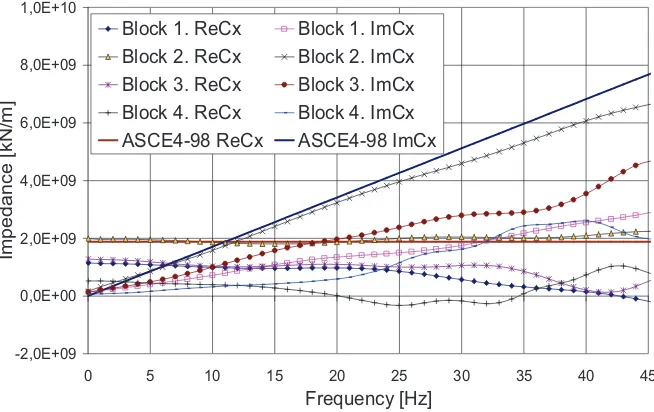
The next step is to obtain impedances and transfer functions from free-field motion to the seismic loads impacting fixed base during seismic event. This analysis was performed by code SASSI (see Lysmer et al. (1981)). For a surface base and vertically propagating seismic waves in horizontally-layered soil the above-mentioned transfer functions to seismic loads are equal to the impedances.

(4)

homogeneous half-space with Vs=1800 m/s, Vp=4100 m/s, density 2,6 t/m3. We see that these ASCE4-98 impedances are not far from the impedances, calculated by SASSI for Block #2.

-2,0E+09 0,0E+00 2,0E+09 4,0E+09 6,0E+09 8,0E+09 1,0E+10

0 5 10 15 20 25 30 35 40 45

Frequency [Hz]

Impe

d

a

n

ce

[

kN/m

]

Block 1. ReCx Block 1. ImCx

ASCE4-98 ReCx ASCE4-98 ImCx

Figure 3. Translational impedances along X-axis

Dynamic Inertia

The next step of the process is a “condensation” of the upper structure to rigid base – for a single–base

structure it means obtaining of the “dynamic inertia” matrix. This calculation is performed only once for four Blocks, as the upper structures are similar. It should be noted, however, that for different levels of seismic excitation these calculations will be different, because internal damping in the structure depends on the excitation level. Here for SL-2 level of excitation material damping for concrete was 7%, and for steel 4%.

Dynamic inertia calculation is based on the results of fixed-base modal analysis performed using ABAQUS. Output of this analysis includes inertial parameters of structure as a rigid body M0 (a real

matrix 6 x 6), list of natural frequencies Ωj together with corresponding modal damping coefficients γj and

also modal participation factors (six factors Sij for each mode j). Dynamic inertia matrix is calculated as

j T j n

j j j j

str

S

i

M

å

=

W

-

+

W

+

=

1

2 2

2

0

2 )

(

wg

w

(1)

The first term in the right-hand part of Equation 1 is a conventional inertia matrix M0 of structure as a rigid body. One can easily obtain it from the data usually provided (e.g., by ABAQUS) after modal fixed-base analysis: total mass of the model; location of the center of mass; moments of inertia about the origin; products of inertia about the origin.

(5)

Division V

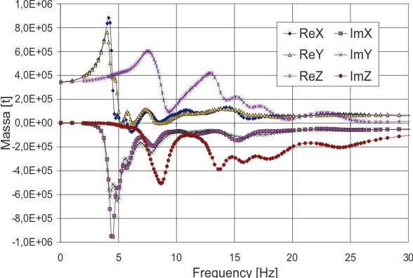
frequencies below 52 Hz. Figure 4 shows dynamic masses along three axes – these are the first three diagonal elements of the complex frequency-dependent dynamic inertia matrix.

For the low frequencies ω dynamic inertia M(ω) comes to the traditional “rigid” inertia M0. “Rigid” masses (unlike dynamic masses) are similar for three translational directions – see Figure 4.

-1,0E+06 -8,0E+05 -6,0E+05 -4,0E+05 -2,0E+05 0,0E+00 2,0E+05 4,0E+05 6,0E+05 8,0E+05 1,0E+06

0 5 10 15 20 25 30

Frequency [Hz]

Massa

[

t]

ReX ImX

ReY ImY

ReZ ImZ

Figure 4. Translational dynamic masses.

Equation of Motion and Transfer Functions

The next step of the process is to combine dynamic stiffness of the soil and dynamic inertia of the structure in the equation of motion for weightless rigid base. Dynamic inertia Mstr for a single-base structure gives the dynamic stiffness Dstr as follows:

) ( )

(w w2 _str w

str M

D =- (2)

Dynamic stiffness of a structure Dstr is simply added to the dynamic stiffness of a soil foundation Dsoil(i.e. to the impedance matrix) leading to the equation of motion in the frequency domain

0

)

(Dstr +Dsoil U =BU (3)

For a surface base the 6 x 3 matrix B is just a part (three first columns) of the 6 x 6 matrix Dsoil . For embedded base it is calculated in a different way.

Equation of motion 3 gives transfer functions from free-field displacement U0 to the rigid base displacement U. This equation is solved in the frequency domain. In our case frequency varied from zero to 40 Hz with 0.5 Hz step. Number of intermediary frequencies was added to catch sharp peaks in transfer functions. For these additional frequencies soil impedances were interpolated between “basic” frequencies, and dynamic inertia was calculated from the beginning. The reason is seen on Figures 3 and 4: soil impedances are rather smooth, and dynamic inertia has sharp peaks.

Transfer functions from U0 to U are calculated in twelve variants (unlike soil impedances calculated in four variants, and unlike dynamic inertia calculated in a single variant). “Soft” and “hard” soil profiles

were obtained from “medium” profile for each Block, using coefficient 1.5 for modules. Poisson’s ratio,

(6)

scaling of impedances. One should apply simultaneous scaling of value G and frequency ω according to the formula

) / ( )

( 2 ₀

1 a G a

G

w

=

w

(4)

Here a2 is a scaling coefficient for modules.

Figure 5 shows absolute values of the transfer functions X(X) for Block # 4 with three soils.

0,0 0,5 1,0 1,5 2,0 2,5

0 5 10 15 20 25 30

Frequency [Hz]

Ab

so

lut

e

va

lue

o

f

tran

sfe

r f

u

n

ctio

n

Block 4. Medium soil

Block 4. Soft soil

Block 4. Hard soil

Figure 5. Transfer functions X(X) for Block #4 with three soils.

Base Response: Time Histories and Spectra

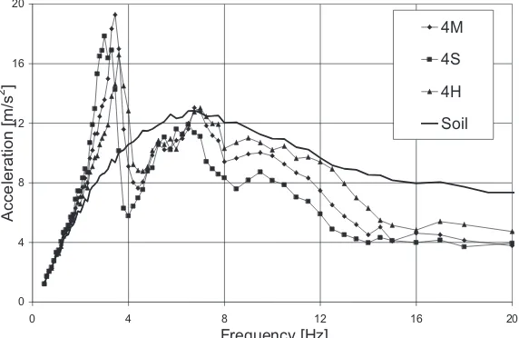
Transfer functions from displacements to displacements and from accelerations to accelerations are similar. They enable calculation of twelve six-component acceleration time histories for rigid base. Calculations are performed using Fast Fourier Transform (FFT). Single three-component free-field time history is used for three soil profiles under each Block as calculated previously by SHAKE (i.e. variation of soil properties is not applied for SHAKE calculations). Figure 6 shows 2% acceleration spectra for Block #4 along X-axis for three soil profiles (M - medium, S - soft, H – hard). They are compared to the free-field spectrum after SHAKE (marked “Soil”).

0 4 8 12 16 20

Frequency [Hz]

Acce

lerat

ion

[

m/s

2 ]

4M

4S

4H

(7)

Division V

Figure 6. Spectra (2% damping) along X-axis for Block #4 with three soils: soft (S), medium (M) and hard (H).

Base Response: Enveloping and Smoothening. Synthesis of Acceleration Time Histories

Figure 7 shows the comparison of corresponding spectra for all four Blocks (each of four spectra is a result of formal pre-enveloping over three soil profiles).

0 4 8 12 16 20

Frequency [Hz]

Acce

lerat

ion

[

m/s

2 ]

Block1

Block2

Block3

Block4

Figure 7. Spectra (2% damping) along X-axis for four blocks pre-enveloped over three soils each.

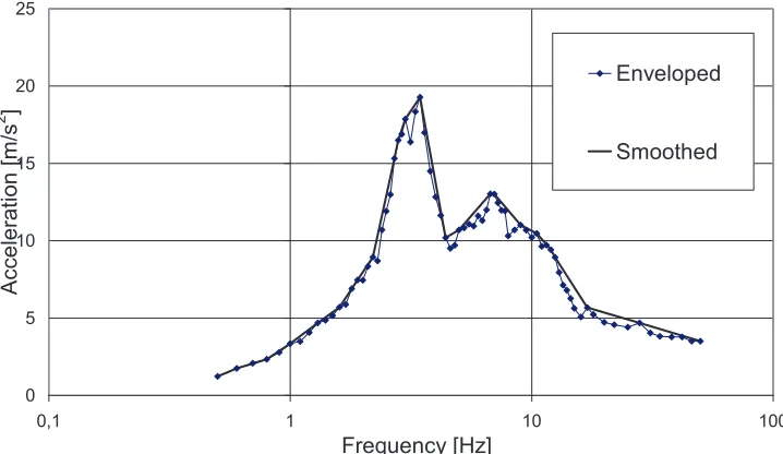
However, enveloping is not so formal. When standard ASCE4-98 requires the variation of the soil profiles, it implicitly requires not only extreme deviations, but all intermediary deviations too. That means that enveloping of spectra from three soil profiles of the same Block must go together with smoothening over all peaks. On the contrary, enveloping of spectra from different Blocks does not require smoothening.

In practice smoothening was performed after formal enveloping. Figure 8 shows the result of smoothening: base acceleration spectra along X-axis before and after smoothening are compared to each other.

0 5 10 15 20 25

0,1 1 10 100

Frequency [Hz]

Acce

lerat

ion

[

m/s

2 ]

Enveloped

(8)

Figure 8. Spectra (2% damping) along X-axis: before and after smoothening procedure.

Next goes the evaluation of “enveloped” time history matching “enveloped” (and smoothed) spectra. In

our example, as it is seen from Figure 6 and Figure 7, many “partial spectra” contribute to the enveloped spectrum. So the only way is to generate a new time history matching enveloped response spectrum. Code AGA (see Tropp (1981)) was used for this purpose.

Check of Conservatism for Different Combination Rules

After 6D “enveloped” base excitation is obtained one should decide how to apply it in order to get conservative results for the upper structure. The main difficulty arises from the fact that during enveloping we lost the correlation between different components of the base response. If no SSI occurs, three components of the base motion taken from the free field are more or less statistically independent. However, in SSI this correlation is important because main response to the horizontal seismic excitation goes in the sway-rocking modes; so for the high elevations the response to the rocking motion of the basement goes along with the response to the horizontal motion of the basement. As a result, the combination of the responses should be closer to the direct sum than to the statistical sum of the independent processes (of the SRSS type).

The author has compared different options in the format of response acceleration spectra (2% damping) in the certain node in the upper structure (in the containment shell at elevation about 53 meters). The first option was the single-analysis response to the 6D enveloped excitation obtained via the algorithm proposed above. The second option was traditional plain enveloping of the nodal response spectra got from twelve separate analyses with different soil conditions (without frequency broadening of response spectra). This option is used as a benchmark.

The third option was called “special sum”. The following formula was used to combine the responses to

1D “enveloped” excitations applied one by one at the rigid base:

2 / 1 2 2 2 2

]

)

(

)

[(

X

YY

Y

XX

Z

ZZ

S

=

+

(5)

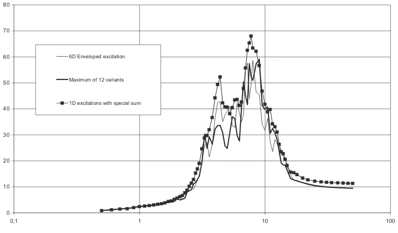
Here X, Y, etc. mean responses to 1D component along X, Y, etc. “Response” means spectral acceleration at a given frequency with a given damping in oscillators. Equation 5 is different from conventional SRSS, because X and YY are combined directly, as well as Y and XX. The comparison of three options is shown on Figure 9 for nodal response spectra along Y and on Figure 10 – for response spectra along vertical Z.

The first conclusion is that the response to the 6D “enveloped” excitation is not always conservative as

compared to the benchmark response. Note that for the horizontal response non-conservatism occurs at low frequencies where dominant sway-rocking modes contribute considerably and correlation is strong. For vertical response non-conservatism appears at higher frequencies. Selected node is far from the central vertical axis, so rocking contributes to vertical nodal response.

The second conclusion is that “special sum” provides conservative results. However, six components of

the base excitation in this case are to be applied one by one in order to get separate responses and to use Equation 5. Note that these six separate analyses are better than six SSI analyses with different soil environment because six 1D excitations are applied to one and the same system (e.g., calculations of eigenfrequencies and modes can be performed only once).

(9)

Division V

broadened nodal response spectra implicitly account for broadened excitations for “extreme soils”. Can it help with the non-conservatism discussed above?

0 10 20 30 40 50 60 70 80 90 100

0,1 1 10 100

Frequency, Hz

6D Enveloped excitation

Maximum of 12 variants

1D excitations with special sum

Figure 9. Comparison of the nodal response spectra (2% damping in oscillators) along Y axis.

0 10 20 30 40 50 60 70 80

0,1 1 10 100

Frequency, Hz

1D excitations with special sum

Figure 10. Comparison of the nodal response spectra (2% damping in oscillators) along Z axis.

(10)

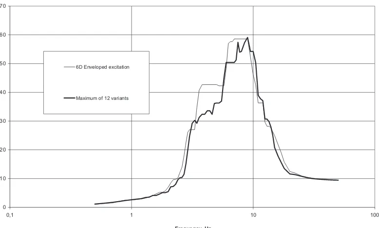
The comparison is shown on Figure 11 for nodal response spectra along Z. Non-conservatism has really become less, but is still present. So, the author still recommends six-analyses procedure with 1D

“enveloped” base excitation and special combination of the responses using Equation 5.

0 10 20 30 40 50 60 70

0,1 1 10 100

Frequency, Hz

Figure 11. Comparison of the nodal response spectra with partial broadening (2% damping in oscillators) along Z axis.

CONCLUSIONS

If several variants of soil foundation are to be analyzed with one and the same structure in SSI problem,

one can use “enveloping” procedure to save resources. However, this enveloping must be performed at the

base level, not at the free surface of the soil foundation. The proposed procedure does not account for the correlation between different components of the base motion (e.g., horizontal and rocking responses). As a result, the response of the upper structure to the “enveloped” 6D base excitation is not always conservative. The author has proposed to obtain the responses to the six components of the “enveloped” base excitation separately, and then combine them using special rule (mixture of SRSS and direct sum).

REFERENCES

American Society of Civil Engineers. (1999). Seismic Analysis of Safety-Related Nuclear Structures and Commentary.ASCE4-98. Reston, Virginia, USA.

Dassault Systèmes Simulia Corp. (2008) ABAQUS. Version 6.8.., Providence, RI, USA.

Lysmer, J., Tabatabaie, R., Tajirian, F., Vahdani, S. and Ostadan, F. (1981) SASSI - A System for Analysis of Soil-Structure Interaction. Research Report GT 81-02. University of California, Berkeley, USA. Schnabel, P.B., Lysmer, J. and Seed, H.B. (1972) SHAKE - a Computer Program for Earthquake

Response Analysis of Horizontally Layered Sites. Rep. EERC 72-12. Berkeley, California, USA. Tropp, R. (1981) AGA. Artificial Generation of Accelerograms. SIEMENS-KWU, Germany.

Tyapin, A.G. (2010) “Combined Asymptotic Method for Soil-Structure Interaction Analysis” // Journal of Disaster Research. 5, 4, 340-350.

Tyapin, A. (2012). “Soil-Structure Interaction”, Earthquake Engineering, Halil Sezen (Ed.), ISBN: