Experimental design for vector output systems

(1)

Experimental Design for Vector Output Systems

H.T. Banks and K.L. Rehm

Center for Research in Scientific Computation Center for Quantitative Sciences in Biomedicine

N.C. State University Raleigh, NC

April 30, 2012

Abstract

We formulate an optimal design problem for the selection of best states to observe and op-timal sampling times for parameter estimation or inverse problems involving complex nonlinear dynamical systems. An iterative algorithm for implementation of the resulting methodology is proposed. Its use and eﬃcacy is illustrated on two applied problems of practical interest: (i) dynamic models of HIV progression and (ii) modeling of the Calvin cycle in plant metabolism and growth.

(2)

1 Introduction

In many scientific fields where mathematical modeling is utilized, mathematical models grow in-creasingly complex, containing possibly more state variables and parameters, over time as the underlying governing processes of a system are better understood and refinements in mechanisms are considered. Additionally, as technology invents and improves devices to measure physical and biological phenomena, new data become available to inform mathematical modeling efforts. The world is approaching an era in which the vast amounts of information available to researchers may be overwhelming or even counterproductive to efforts. We explore a framework based on the Fisher Information Matrix (FIM) for a system of ordinary differential equations (ODEs) to determine when an experimenter should take samples and what variables to measure when collecting information on a physical or biological process that is modeled by a dynamical system.

Inverse problem methodologies are discussed in [10] in the context of dynamical system or math-ematical model parameter estimation when a sufficient number of observations of one or more states (variables) are available. The choice of method depends on assumptions the modeler makes on the form of the error between the model and the observations (the statistical model). The most preva-lent source of error is observation error, which is made when collecting data. (One can also consider model error, which originates from the differences between the model and the underlying process that the model describes. But this is often quite difficult to quantify.) Measurement error is most readily discussed in the context of statistical models. The three techniques commonly addressed are maximum likelihood estimators (MLE), used when the properties of the error distribution are known; ordinary least squares (OLS), for error with constant variance across observations; and generalized least squares (GLS), used when the variance of the data can be expressed as a noncon-stant function. Uncertainty quantification is also described for optimization problems of this type, namely in the form of observation error covariances, standard errors, residual plots, and sensitivity matrices. Techniques to approximate the variance of the error are also included in these discussions. Experimental design using the Fisher Information Matrix (FIM), which is based on sensitivity matrices, is described in [11] for the case of scalar data. Sensitivity matrices are composed of functions that relate the change in a variable to the change in the parameter. The first order quan-tifications of these relations are called traditional sensitivity functions and are useful in suggesting when a variable should be sampled to get the most information for estimating a particular param-eter, especially when the first order sensitivity functions are used in conjunction with the so-called second order sensitivity functions. This work also examines the usefulness of generalized sensitivity functions [18], which are calculated using the FIM, that are known to describe how information about the parameters is distributed across time for each variable. Both types of sensitivity func-tions are then used in numerical simulafunc-tions to determine the optimal final time for an experiment of a process described by a logistic curve.

In [12], the authors develop an experimental design theory using the FIM to identify optimal sampling times for experiments on physical processes (modeled by an ODE system) in which scalar or vector data will be taken. The experimental design technique developed is applied in numerical simulations to the logistic curve, a simple ODE model describing glucose regulation and a harmonic oscillator example.

(3)

output of interest at any one particular time. A model using a subset of variables is determined via multivariate linear regression, and the efficacy of the model is then measured using the Akaike Information Criterion. The variables that appear in the best models at the most time points are then identified as the most important to measure. Such a method does not utilize the information on the underlying time-varying processes given by the dynamical system model. Extension of the second method first suggested in [5], based optimal design ideas, is the subject of our presentation here.

Building on the theory in [12] and [5], we formulate a previously unexplored optimal design problem to determine not only the optimal sampling variables out of a finite set of possible sampling variables but also the optimal sampling time distribution given a fixed final time. We compare the Soptimal design introduced in [11] and [12] with the well-known methods of D-optimal and E-optimal design on a six-compartment HIV model [2] and a thirty-one dimensional model of the Calvin Cycle [19]. Such models where there may be a wide range of variables to possibly observe are not only ideal on which to test our proposed methodology, but also are widely encountered in applications.

2 Mathematical Background

2.1 Mathematical and statistical models

We explore our experimental design questions using amathematical model

d⃗x

dt(t) = ⃗g(t, ⃗x(t;

⃗

θ), ⃗q), t∈[t0, tf] (1)

⃗

x(t0;⃗θ) = ⃗x0

where ⃗x(t;⃗θ) is the vector of state variables of the system generated using a parameter vector ⃗

θ= (⃗x0;⃗q)∈Rp, p=m+r, that contains m initial values and r system parameters listed in ⃗q,⃗g

is a mappingR1+m+r →Rm,t0 ≥0 is the initial time, and tf <∞is the ﬁnal time. We deﬁne an observation process

⃗

f(t;⃗θ) =C⃗x(t;⃗θ), (2)

where C is an observation operator that maps Rm → RN, where N is the number of variables observed at a single sampling time. If we were able to observe all states, each measured by a diﬀerent sampling technique, thenN =mand C=Im×m; however, this is most often not the case because of the impossibility of or the expense in measuring all state variables. In other cases (such as the HIV example below) we may be able to directly observe only combinations of the states.

In order to discuss the amount of uncertainty in parameter estimates, we formulate astatistical model[10] of the form

⃗

Y(t) =f⃗(t;⃗θ0) +E⃗(t), t∈[t0, tf], (3)

where ⃗θ0 is the hypothesized true values of the unknown parameters and E⃗ is a vector random

(4)

E(E⃗(t)) = ⃗0, t∈[t0, tf],

Var(E⃗(t)) = V0(t) = diag(σ0,1(t)2, σ0,2(t)2, . . . , σ0,N(t)2), t∈[t0, tf],

Cov(Ei(t)Ei(s)) = σ0,i(t)2δ(t−s), s, t∈[t0, tf],

Cov(Ei(t)Ej(s)) = 0, i̸=j, s, t∈[t0, tf],

whereδ(0) = 1 andδ(t) = 0 for t̸= 0. Realizations of the statistical model (3) are written

⃗

y(t) =f⃗(t;⃗θ0) +⃗ϵ(t), t∈[t0, tf].

When collecting experimental data, it is often diﬃcult to take continuous measurements of the observed variables. Instead, we assume that we have n observations at times tj, j = 1, . . . , n,

t0≤t1< t2 < . . . < tn≤tf. We then write the observation process (2) as

⃗

f(tj;⃗θ) =C⃗x(tj;⃗θ), j = 1,2, . . . , n, (4)

the discrete statistical model as

⃗

Yj =f⃗(tj;⃗θ0) +E⃗(tj), j= 1,2, . . . , n, (5)

and a realization of the discrete statistical model as

⃗yj =f⃗(tj;⃗θ0) +⃗ϵ(tj), j = 1,2, . . . , n.

If we were given ⃗θ0, we could solve (1) for ⃗x(t;⃗θ0), a process known as solving the forward problem. Alternatively, if we had a set of data⃗yj,j = 1,2, . . . , n, we could estimate⃗θ0 in a process

known as solving theinverse problem. We will use this mathematical and statistical framework to develop a methodology to identify sampling variables that provide the most information pertinent to estimating a given set of parameters and the most informative times at which the samples should be taken.

2.2 Formulation of the Optimal Design Problem

Several methods exist to solve the inverse problem. A major factor [10] in determining which method to use is additional assumptions made aboutE⃗(t). It is common practice to make the assumption that realizations ofE⃗(t) at particular time points are independent and identically distributed (i.i.d.). If, additionally, the distributions describing the behavior of the components ofE⃗(t) are known, then maximum likelihood methods may be used to ﬁnd an estimate of ⃗θ0. On the other hand, if the

distributions for E⃗(t) are not known but the variance V0(t) (also unknown) is assumed to vary

over time, weighted least squares methods are often used. We propose an optimal design problem formulation using a generalized weighted least squares criterion.

Let P1([t0, tf]) denote the set of all bounded distributions on the interval [t0, tf]. We consider

the generalized weighted least squares cost functional for systems with vector output

JW LS(⃗y, ⃗θ) =

∫ tf

t0

[⃗y(t)−f⃗(t;⃗θ)]TV₀−1(t)[⃗y(t)−f⃗(t;⃗θ)]dP1(t), (6)

(5)

We next consider the case of observations collected at discrete times. If we choose a set of n time pointsτ ={tj},j= 1,2, . . . , n, where t0≤t1 < t2 < . . . < tn≤tf and take

P(t) =Pτ =

n

∑

j=1

δtj, (7)

where δa represents the Dirac delta distribution with atom at a, then the weighted least squares

criterion (6) for a ﬁnite number of observations becomes

J_{W LS}n (⃗y, ⃗θ) =

n

∑

j=1

[⃗y(tj)−f⃗(tj;⃗θ)]TV0−1(tj)[⃗y(tj)−f⃗(tj;⃗θ)].

To select a useful distribution of time points and set of observation variables, we introduce the N by p sensitivity matrices

[

∂ ⃗f(t;⃗θ) ∂⃗θ

]

and the m by p sensitivity matrices

[

∂⃗x(t;⃗θ) ∂⃗θ

]

that are

determined using the diﬀerential operator in row vector form (∂θ1, ∂θ2, . . . , ∂θp) represented by ∇⃗_θ

and the observation operator deﬁned in (2),

∇⃗_θf⃗(t, ⃗θ) =

∂ ⃗f(t;⃗θ)

∂⃗θ

= C∂⃗x(t;⃗θ)

∂⃗θ = C       

∂x1(t;⃗θ)

∂θ1

∂x1(t;⃗θ)

∂θ2 . . .

∂x1(t;⃗θ)

∂θp ∂x2(t;⃗θ)

∂θ1

∂x2(t;⃗θ)

∂θ2 . . .

∂x2(t;⃗θ)

∂θp

..

. ... . .. ...

∂xm(t;θ⃗) ∂θ1

∂xm(t;⃗θ)

∂θ2 . . .

∂xm(t;⃗θ) ∂θp       

= C∇⃗_θ⃗x(t;⃗θ). (8)

Using the sensitivity matrix ∇⃗_θf(t, ⃗θ0), we may formulate the Generalized Fisher Information

Matrix (GFIM). Consider the set C ⊂Rm of admissible observation maps and letP2(C) represent the set of all bounded distributionsP2(c) onC. Then the GFIM may be written

F(P1, P2, ⃗θ0) ≡

∫ tf

t0

∫

C

1

σ2₍_{t, c}₎∇⃗θ

T_f_⃗₍_t_;_⃗_θ

0)∇⃗_θf⃗(t;⃗θ0)dP2(c)dP1(t) (9)

=

∫ tf

t0

∫

C

1

σ2₍_{t, c}₎∇⃗θ

T(_c⃗_x₍_t_;_⃗_θ

0)

)

∇⃗_θ

(

c⃗x(t;⃗θ0)

)

dP2(c)dP1(t). (10)

Taking N diﬀerent sampling maps in C represented by the m-dimensional row vectors ck,k=

1,2, . . . , N, we construct the discrete distribution onC

PC =

N

∑

k=1

δck, (11)

where δa represents the Dirac delta distribution with atom at a. Using PC in (10), we obtain the

(6)

F(P1, PC, ⃗θ0) =

∫ tf

t0

N

∑

k=1

1

σ2₍_{t, c}

k)∇⃗θ

T(_c

k⃗x(t;⃗θ0)

)

∇⃗_θ

(

ck⃗x(t;⃗θ0)

)

dP1(t)

=

∫ tf

t0

N

∑

k=1

1

σ2₍_{t, c}

k)

∇⃗_θT⃗x(t;⃗θ0)ckTck∇⃗_θ⃗x(t;⃗θ0)dP1(t)

=

∫ tf

t0

N

∑

k=1

∇⃗_θT⃗x(t;⃗θ0)ckT

1

σ2₍_{t, c}

k)

ck∇⃗_θ⃗x(t;⃗θ0)dP1(t)

=

∫ tf

t0

∇⃗_θT⃗x(t;⃗θ0) N

∑

k=1

(

ckT

1

σ2₍_{t, c}

k)

ck

)

∇⃗_θ⃗x(t;⃗θ0)dP1(t)

=

∫ tf

t0

∇⃗_θT⃗x(t;⃗θ0)

(

CTV₀−1(t)C

)

∇_θ⃗⃗x(t;θ⃗0)dP1(t), (12)

whereC = (c1, c2, . . . , cN)T ∈RN×m is the observation operator in (2) and (4) andV0(t)∈RN×N

is the covariance matrix as described in (3). Applying the distribution Pτ as described in (7) to

the GFIM (12) for discrete observation operators measured continuously yields the discrete p×p Fisher Information Matrix (FIM) for discrete observation operators measured at discrete times

F(τ, C, ⃗θ0) =F(Pτ, PC, ⃗θ0) =

n

∑

j=1

∇⃗_θT⃗x(tj;⃗θ0)CTV0−1(tj)C∇⃗_θ⃗x(tj;⃗θ0). (13)

This describes the amount of information about the p parameters of interest that is captured by the observed quantities described by the sampling mapsck,k= 1,2, . . . , N, listed inC, when they

are measured at the time points in τ.

The questions of determining the best (in some sense) C and τ are important questions in the optimal design of an experiment. Recall that the set of time points τ has an associated distribution P1(τ) =Pτ ∈ P1([t0, tf]), where P1([t0, tf]) is the set of all bounded distributions on

[t0, tf]. Similarly, the set of sampling maps {ck} has an associated bounded distribution PC ∈ P2(C). Deﬁne the space of bounded distributionsP([t0, tf]×C) =P1([t0, tf])×P2(C) with elements

P = (Pτ, PC) ∈ P. Without loss of generality, assume that C ⊂ Rm is closed and bounded, and

assume that there exists a functionalJ :Rp×p→R+of the GFIM (10). Then theoptimal design problemassociated withJ is selecting a distribution ˆP ∈ P such that

J (F( ˆP , ⃗θ0)

)

= min

P∈PJ

(

F(P, ⃗θ0)

)

, (14)

whereJ depends continuously on the elements of F(P, ⃗θ0).

The Prohorov metric [16] provides a general theoretical framework for the existence of ˆP and approximation in P([t0, tf]× C) (a general theoretical framework is developed in [7, 11]). The

application of the Prohorov metric to optimal design problems formulated as (14) is explained more fully in [11]: brieﬂy, deﬁne the Prohorov metric ρ on the space P([t0, tf]× C), and consider

the metric space (P([t0, tf]× C), ρ). Since [t0, tf]× C is compact, (P([t0, tf]× C), ρ) is also compact.

Additionally, by the properties of the Prohorov metric, (P([t0, tf]×C), ρ) is complete and separable.

(7)

the form of J. Each of these design criteria are functions of the inverse of the FIM (assumed hereafter to be invertible) deﬁned in (13).

In D-optimal design, the cost functional is written

JD(F) = det

(

F(τ, C, ⃗θ0)−1

)

= 1

det

(

F(τ, C, ⃗θ0)

).

By minimizing JD, we minimize the volume of the conﬁdence interval ellipsoid describing the

uncertainty in our parameter estimates. SinceF is symmetric and positive semi-deﬁnite,JD(F)≥

0. Additionally, since F is assumed invertible, JD(F)̸= 0, therefore,JD :Rp×p→R+.

In E-optimal design, the cost functional is JE is the largest eigenvalue of

(

F(τ, C, ⃗θ0)

)₋1

, or equivalently

JE(F) = max

1

eig

(

F(τ, C, ⃗θ0)

).

To obtain a smaller standard error, we must reduce the length of the principal axis of the conﬁdence interval ellipsoid. Since an eigenvalueλsolves det(F−λI) = 0, an eigenvalue ofλ= 0 would mean det(F) = 0, or that F is not invertible. Since F is positive deﬁnite, all eigenvalues are therefore positive. ThusJE :Rp×p →R+.

In SE-optimal design,JSEis a sum of the elements on the diagonal of

(

F(τ, C, ⃗θ0)

)₋1

weighted

by the respective parameter values [11, 12], written

JSE(F) = p

∑

i=1

(

F(τ, C, ⃗θ0))

)₋1 i,i

θ2

0,i

.

Thus in SE-optimal design, the goal is to minimize the sum of squared errors of the parameters normalized by the true parameter values. As the diagonal elements of F−1 are all positive and all parameters are assumed non-zero in⃗θ∈Rp,JSE :Rp×p →R+.

In [12], it is shown that the D-, E-, and SE-optimal design criteria select different time grids and yield different standard errors. We expect that these design cost functionals will also choose different observation variables (maps) in order to minimize different dimensions of the confidence interval ellipsoid.

3 Algorithm and optimization constraints

In most optimal design problems, there is not a continuum of measurement possibilities that may be used; rather, there are N∗<∞ possible observation mapsc. Denote this set as CN∗ ⊂Rm. While

we may still use the Prohorov metric-based framework to guarantee existence and convergence of (14), we have a stronger result ﬁrst proposed in [5] that is useful in numerical implementation. Because CN∗ is ﬁnite, all probability distributions made from the elements of CN∗ have the form

P2({ck}) =PC =

∑N

k=1δck for a ﬁxedN. Moreover, the set of all distributions that useN sampling

methodsP₂N(CN∗) is also ﬁnite. For a ﬁxed distribution of time pointsPτ, we may compute using

(13) the set of all possible FIM F(Pτ, PC, ⃗θ) that could be formulated from c ∈ CN∗. By the

(8)

time pointsPτ, we may ﬁnd at least one solution ˆPC ∈ P2N(CN∗). Moreover, ˆPC may be determined

by a search over all matricesC = (c1, c2, . . . , cN)T formed by N elements from CN∗.

Due to the computational demands of performing nonlinear optimization forntime points and N observation maps (for a total ofn+N dimensions), we instead solve the coupled set of equations

ˆ

C= argmin

{C|PC∈P2N(CN∗)}

J (F(ˆτ , C, ⃗θ0)

)

(15)

ˆ

τ = argmin

{τ|Pτ∈P1([t0,tf])}

J (F(τ,C, ⃗ˆ θ0)

)

, (16)

whereC ∈RN×m _{represents a set of}_N _{sampling maps and}_τ ₌_{_t

j}nj=1,t0≤t1< t2 < . . . < tn≤

tf, is an ordered set of nsampling times. These equations are solved iteratively as

ˆ

Ci = argmin

{C|PC∈P2N(CN∗)}

J (F(ˆτi−1, C, ⃗θ0)

)

(17)

ˆ

τi= argmin {τ|Pτ∈P1([t0,tf])}

J (F(τ,Cˆi, ⃗θ0)

)

, (18)

whereJ is the D-, E-, or SE-optimal design criterion. We begin by solving for ˆC1where ˆτ0 is

speci-ﬁed by the user. The system (17)-(18) is solved until|J

(

F(ˆτi,Cˆi, ⃗θ0)

)

−J (F(ˆτi−1,Cˆi−1, ⃗θ0)

)

|< ϵ

or until ˆCi= ˆCi−1. For each iteration, (17) is solved using a global search over all possibleC. Since

the sensitivity equations cannot be easily solved for in the models chosen to illustrate our method, we use a modiﬁed version of tssolve.m by A. Attarian [4], which implements the myAD package developed by M. Fink [14]. Solving (18) requires using a nonlinear constrained optimization algo-rithm. While MATLAB’s fmincon is a natural choice for such problems, as reported in [12], it does not perform well in this situation. Instead, we use SolvOpt developed by A. Kuntsevich and F. Kappel [15]. We select for our use two of the four variations on the constraint implementation used in [12]. Following the numbering in [12], the constraints are

(C2) In the second constraint scheme used by [12], the initial and ﬁnal time points are ﬁxed as t1 = t0 and tn = tf. The routine optimizes over the remaining n−2 time points such that

tj ≤tj+1.

(C3) In the third constraint scheme used by [12], we instead optimize the time steps νj ≥0. We

ﬁx t1 = t0 and tn = tf, and the remaining time points may be found by tj+1 = tj +νj,

j = 1,2, . . . , n−2. Additionally, tf −t0 ≥

∑n−2

j=1νj. This routine also optimizes over n−2

variables.

Once either of the convergence requirements are met and ˆC and ˆτ are determined, we compute standard errors using the asymptotic theory described in the next section.

4 Standard Errors

(9)

the three previously described optimal design methods, we compute the standard errors for the parameters in ⃗θ. There are multiple techniques [12] available to compute standard errors; here we choose to use asymptotic theory due to its ease of implementation.

4.1 Asymptotic Theory for Standard Errors

If we assume that the covariance matrix V0(t) is constant over time (V0(t) ≡ V0 = Var(E⃗(tj)) =

diag(σ2₀_,₁, σ₀2_,₂, . . . , σ₀2_,N)), then we may use an ordinary least squares (OLS) framework to estimate standard errors. Once an optimalτ ={tj}Nj=1,t0≤t1< t2 < . . . < tn≤tf, andCare determined,

we obtain data from an experiment or simulate data {yj} as a realization of the random process {Yj} described in (5), and then we estimate the parameters in ⃗θ by solving the inverse problem

using the OLS criterion [10]. The discrete OLS estimator is deﬁned as

⃗

θOLS= argmin

⃗ θ∈Θ n ∑ j=1 [ ⃗

Yj−f⃗(tj;⃗θ)

]T

V₀−1

[ ⃗

Yj−f⃗(tj;⃗θ)

]

, (19)

where Θ is the set of all possible values of ⃗θ, such that each element of the diﬀerence vector ⃗

Yj−f⃗(tj;⃗θ) is weighted using the variance of its corresponding sampling maps. One realization of

this problem using data⃗yj,j= 1,2, . . . , n, is written

ˆ

θOLS = argmin

⃗ θ∈Θ n ∑ j=1 [ ⃗

yj−f⃗(tj;⃗θ)

]T

V₀−1

[ ⃗

]

. (20)

However, calculating ˆθOLS still requires the unknown V0. If the number of parameters p of a

system is suﬃciently small and number of observationsnlarge so thatp < n, then we may calculate the bias adjusted estimate of the variances

V0 ≈Vˆ = diag



 1

n−p

n

∑

j=1

[ ⃗

] [ ⃗

yj−f⃗(tj;θ⃗)

]T



, (21)

and ﬁnd the estimate of ⃗θ0 using

⃗

θ0 ≈θˆOLS= argmin

⃗ θ∈Θ n ∑ j=1 [ ⃗

yj −f⃗(tj;⃗θ)

]T

ˆ

V−1

[ ⃗

yj −f⃗(tj;⃗θ)

]

. (22)

Therefore, ﬁnding ˆθOLS when V0 is unknown requires solving the coupled system of equations (21)

and (22).

We may utilize the asymptotic properties of the OLS minimizer (19) to learn about the behavior of the model (1) and (3). As the number of samples n → ∞, ⃗θOLS has the following properties [10, 13, 17]

⃗

θOLS ∼ N(⃗θ0,Σn0)≈ N(ˆθOLS,Σˆn),

where

Σn₀ ≈

 ∑n

j=1

χ_jT(⃗θ0)V0−1χj(⃗θ0)

 

−1

(10)

is the p×pcovariance matrix, and χj(⃗θ) =χnj(⃗θ) =∇⃗_θf⃗(tj;⃗θ0) is the N×pmatrix

χj(⃗θ) =χnj(⃗θ) =

    

∂f1(tj;⃗θ)

∂θ1

∂f1(tj;⃗θ)

∂θ2 . . .

∂f1(tj;⃗θ)

∂θp

..

. ... ...

∂fN(tj;⃗θ) ∂θ1

∂fN(tj;θ⃗)

∂θ2 . . .

∂fN(tj;⃗θ) ∂θp

   

. (24)

The approximation ˆΣn to the covariance matrix Σn₀ is

Σn₀ ≈Σˆn=

 ∑n

j=1

χT_j(ˆθOLS) ˆV−1χj(ˆθOLS)

 

−1

. (25)

We may use ˆΣn to approximate the standard errors of each parameter in ˆθOLS. For the kth element of ˆθOLS, written ˆθOLS,k, the asymptotic standard error is

ASE(⃗θ0,k) =

√

ˆ Σn

0,kk ≈ASE(ˆθOLS,k) =

√

ˆ Σn

kk,

where ˆΣn₀_,kk is the element in the kth row and kth column of Σn₀, and ˆΣn_kk is the corresponding element in ˆΣn. Additionally, since the FIM is deﬁned to be the inverse of the covariance matrix, we may approximate the FIM using (25) by F(τ, C, ⃗θ0)≈F(ˆτ ,C,ˆ θˆOLS) = ( ˆΣn)−1.

5 Example 1: HIV model

After validating code results for time point selection on simple models such as those in [12], we examined the performance of both the time point and observable operator selection algorithms on the log-scaled version of the HIV model developed in [1]. While the analytic solution of this system cannot easily be found, this model has been studied, improved, and successfully ﬁt to and indeed validated with several sets of longitudinal data using parameter estimation techniques [2, 3]. Additionally, the sampling or observation operators used to collect data in a clinical setting as well as the relative usefulness of these sampling techniques are known [2]. The model includes uninfected and infected CD4+T-cells, called type 1 target cells (T1andT1∗, respectively), uninfected

and infected macrophages (subsequently determined to more likely be resting or inactive CD4+ T-cells), called type 2 target cells (T2 and T2∗), infectious free virus VI, and immune response E

produced by cytotoxic T-lymphocytes CD8+. The HIV model with treatment function u(t) is given by

˙

T1 = λ1−d1T1−(1−ϵ1u(t))k1VIT1

˙

T2 = λ2−d2T2−(1−f ϵ1u(t))k2VIT2

˙

T₁∗ = (1−ϵ1u(t))k1VIT1−δT1∗−m1ET1∗

˙

T₂∗ = (1−f ϵ1u(t))k2VIT2−δT2∗−m2ET2∗ (26)

˙

V = NTδ(T1∗+T2∗)−[c+ (1−ϵ2u(t))103k1T1+ (1−f ϵ1u(t))103k2T2]VI

˙

E = λE+bE

T₁∗+T₂∗

T₁∗+T₂∗+Kb

E−dE

T₁∗+T₂∗

T₁∗+T₂∗+Kd

(11)

The log-scaled HIV model, which is used to alleviate diﬃculties due to the large diﬀerences in scales of the variables and the parameters, is

˙

x1 =

10−x1 ln(10)

(

λ1−d110x1 −(1−ϵ1u(t))k110x1+x5

)

˙

x2 =

10−x2 ln(10)

(

λ2−d210x2 −(1−f ϵ1u(t))k210x5+x2

)

˙

x3 =

10−x3 ln(10)

(

(1−ϵ1u(t))k110x5+x1−δ10x3 −m110x6+x3

)

˙

x4 =

10−x4 ln(10)

(

(1−f ϵ1u(t))k210x5+x2−δ10x4 −m210x6+x4

)

(27)

˙

x5 =

10−x5 ln(10)

(

(1−ϵ2u(t))103NTδ(10x3+ 10x4)−c10x5

−(1−ϵ1u(t))ρ1103k110x1+x5−(1−f ϵ1u(t))ρ2103k210x2+x5

)

˙

x6 =

10−x6 ln(10)

(

λE+

bE(10x3+ 10x4)

10x3_{+ 10}x4 ₊_K

b

10x6− dE(10

x3 _{+ 10}x4₎

10x3 _{+ 10}x4 ₊_K

d

10x6 −_δ

E10x6

)

, (28)

whereT1= 10x1,T2= 10x2,T1∗ = 10x3,T2∗ = 10x4,VI = 10x5, andE = 10x6.

In [2] this model’s parameters are estimated for each of 45 diﬀerent patients who were in a treat-ment program for HIV at Massachusetts General Hospital (MGH). These individuals experienced interrupted treatment schedules, in which the patient did not take any medication for viral load control. Seven of these patients adhered to a structured treatment interruption schedule planned by the clinician. We use the parameters estimated to ﬁt the data of one of these patients, Pa-tient 4 in [2], as our “true” parameters ⃗θ0 for this model. This patient was chosen because the

patient continued treatment for an extended period of time (1919 days) and the corresponding data set contains 158 measurements of viral load and 107 measurements of CD4 cell count (T1+T1∗)

that exhibit a response to interruption in treatment, and the estimated parameters yield a model exhibiting trends similar to that in the data.

Sensitivity analysis performed in [1] and parameter subset selection carried out in [8] identiﬁed subsets of the 20 parameters and six initial conditions that would likely be reliably estimated when solving the corresponding inverse problems. Based on their results, we treat the subset of parameters⃗θ= (λ1, d1, ϵ1, k1, ϵ2, NT, c, bE, x01, x02, x05) as unknown and ﬁx all other parameters. The

values for the ﬁxed parameters and ⃗θ0 are computed in [2] and given in Table 1. It is important

to choose parameters to which the model is sensitive; a poor choice for the components of ⃗θ will negatively aﬀect sensitivity matrices and may lead to a near-singular FIM. Based on currently available measurement methods, we allow the possible types of observations including (1) infectious virusx5, (2) immune responsex6, (3) total activated CD4 cells x1+x3, and (4) type 2 (resting or

unactivated) target cellsx2+x4, each with an assumed error variance of 10% of the initial variable

values given by⃗x0 _{= (3}_.₀₇₉₉_,₁_.₂₄₄₃_,₁_.₇₈₉₉_,₋₀_.₂₁₅₀_,₅_.₉₉₈₄_,₋₀_.₇₂₅₁₎T_.

5.1 HIV observable selection results, times fixed

(12)

Table 1: Values of parameters in the HIV model (26).

parameter value unit parameter value unit

λ1 4.633 _µ_ml-bloodcells _·_day λ2 0.1001 _µ_ml-bloodcells _·_day

d1 0.004533 _day1 d2 0.02211 _day1

k1 1.976e-6 _virionsml

·day k2 5.529e-4

ml virions·day

ϵ1 100.6017 - ϵ2 100.5403

-m1 0.02439 _cellsµml

·day m2 0.013099 _cellsµml

·day

δ 0.1865 1

day c 19.36

1 day

f 100.53915 _- _N

T 19.04 virions_cell

λE 0.009909 _µ_ml-bloodcells _·_day δE 0.0703 _day1

bE 0.09785 _day1 dE 0.1021 _day1

Kb 0.3909 cells

µml-blood Kd .8379

cells µml-blood

the three optimal design criteria, and the asymptotic standard errors (ASE) are calculated after carrying out the corresponding inverse problem calcualtions.

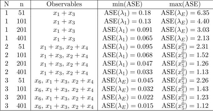
Tables 2, 3, and 4 display the optimal observation operators determined by the D-, E-, and SE-optimal design cost functions, respectively, as well as the lowest and highest ASE. In all three optimal design criteria, there was a distinct best choice of observables (listed in Tables 2, 3, and 4) for each pair of n and N. When only N = 1 observable could be measured, each design criterion consistently picked the same observable for all n; similarly, atN = 2, both the D-optimal and SE-optimal design criteria were consistent in their selection over all n, and E-optimal only diﬀered at n= 401. Even atN = 3, each optimal design method speciﬁed at least two of the same observables at all n.

The observables that were rated best changed between criteria, aﬃrming the fact that each optimal design methods minimizes diﬀerent aspects of the standard error ellipsoid. At N = 1 observable, D-optimal selects the CD4 cell count while E-optimal and SE-optimal choose the infec-tious virus count. As a result, the min(ASE) calculated for a parameter estimation problem using the D-optimal observables is approximately 1/3 lower than the min(ASE) of E- and SE-optimal for all tested time point distributions. Similarly, the max(ASE) calculated for E- and SE-optimal designed parameter estimation problems is approximately 1/3 lower than that of D-optimal. Thus at N = 1, based on minimum and maximum asymptotic standard errors, there is no clear best choice of an optimal design cost function.

(13)

Table 2: Number of observables, number of time points, observables selected by D-optimal cost functional, and the minimum and maximum standard error and associated parameter for the pa-rameter subset in the HIV model (27).

N n Observables min(ASE) max(ASE)

1 51 x1+x3 ASE(λ1) = 0.18 ASE(λE) = 6.35

1 101 x1+x3 ASE(λ1) = 0.13 ASE(λE) = 4.40

1 201 x1+x3 ASE(λ1) = 0.091 ASE(λE) = 3.03

1 401 x1+x3 ASE(λ1) = 0.065 ASE(λE) = 2.13

2 51 x1+x3,x2+x4 ASE(λ1) = 0.095 ASE(x05) = 2.31

2 101 x1+x3,x2+x4 ASE(λ1) = 0.068 ASE(x05) = 1.52

2 201 x1+x3,x2+x4 ASE(λ1) = 0.047 ASE(x05) = 1.26

2 401 x1+x3,x2+x4 ASE(λ1) = 0.033 ASE(x05) = 1.13

3 51 x6,x1+x3,x2+x4 ASE(λE) = 0.045 ASE(x05) = 2.26

3 101 x6,x1+x3,x2+x4 ASE(λE) = 0.032 ASE(x05) = 1.43

3 201 x6,x1+x3,x2+x4 ASE(λE) = 0.022 ASE(x05) = 1.23

3 401 x6,x1+x3,x2+x4 ASE(λE) = 0.015 ASE(x05) = 1.12

to be reduced, but for the best overall improvement (as measured by percent reduction from the E-optimal ASE), D- and SE-optimal are recommended.

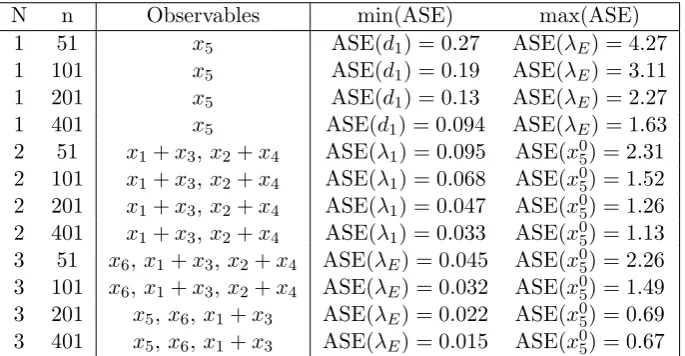
When selecting N = 3 observables, each of the three design criteria select many of the same observables. This is to be expected as N∗ = 4 in this simulation. For n = 51,101,201, both total CD4 cell count and immune response E(t) are selected by all design criteria. The D-optimal criterion also chooses type 2 cell count, so the lack of information on virus count as measured by x5(t) leads to its high max(ASE), ASE(x05). E-optimal (and at larger n, SE-optimal) choose to

measure infectious virus count, reducing ASE(x0₅) and thus reducing the max(ASE) by more than 50%. While at low n, E-optimal has the lowest min(ASE) and max(ASE), SE-optimal performs better at high n, so when selecting N = 3 observables, the number of time points n may aﬀect which optimal design cost function performs best.

5.2 HIV observables and time point selection results

When taking samples on a uniform time grid, D-, E-, and SE-optimal design criteria all choose observation operators that yield favorable ASE’s, with some criteria performing best under certain circumstances. For example, the SE-optimal observables at n = 401, N = 3 yield the smallest standard errors; however, for all other values ofn atN = 3, E-optimal performs best. AtN = 2, E-optimal is a slightly weaker scheme. The examples in [12] also reveal that D-, E-, and SE-optimal designs are all competitive when only selecting time points for several diﬀerent models. Now we wish to investigate the performance of these three criteria when selecting both an observation operator and a sampling time distribution using the algorithm described by equations (17) and (18).

To maintain consistency across trials while slightly simplifying the parameter estimation prob-lem, we allow the set of six parameters and three initial conditions ⃗θ = (λ1, d1, k1, NT, c, bE,

x0₁, x0₂, x0₅) to be treated as unknowns and ﬁx all other parameters. We again allow the possible observations of (1) infectious virusx5, (2) immune responsex6, (3) CD4 cellsx1+x3, and (4) type

2 target cellsx2+x4, each with an assumed error variance of 5% of the initial variable values given

(14)

Table 3: Number of observables, number of time points, observables selected by E-optimal cost functional, and the minimum and maximum standard error and associated parameter for the pa-rameter subset in the HIV model (27).

1 51 x5 ASE(d1) = 0.27 ASE(λE) = 4.27

1 101 x5 ASE(d1) = 0.19 ASE(λE) = 3.11

1 201 x5 ASE(d1) = 0.13 ASE(λE) = 2.27

1 401 x5 ASE(d1) = 0.094 ASE(λE) = 1.63

2 51 x5,x2+x4 ASE(d1) = 0.12 ASE(λE) = 2.18

2 101 x5,x2+x4 ASE(d1) = 0.095 ASE(λE) = 1.52

2 201 x5,x2+x4 ASE(d1) = 0.065 ASE(λE) = 1.10

2 401 x5,x1+x3 ASE(λ1) = 0.042 ASE(λE) = 0.86

3 51 x5,x6,x1+x3 ASE(λE) = 0.045 ASE(x05) = 0.77

3 101 x5,x6,x1+x3 ASE(λE) = 0.032 ASE(x05) = 0.73

3 201 x5,x6,x1+x3 ASE(λE) = 0.022 ASE(x05) = 0.69

3 401 x5,x1+x3,x2+x4 ASE(λ1) = 0.032 ASE(x05) = 0.65

Table 4: Number of observables, number of time points, observables selected by SE-optimal cost functional, and the minimum and maximum standard error and associated parameter for the pa-rameter subset in the HIV model (27).

1 51 x5 ASE(d1) = 0.27 ASE(λE) = 4.27

1 101 x5 ASE(d1) = 0.19 ASE(λE) = 3.11

1 201 x5 ASE(d1) = 0.13 ASE(λE) = 2.27

1 401 x5 ASE(d1) = 0.094 ASE(λE) = 1.63

2 51 x1+x3,x2+x4 ASE(λ1) = 0.095 ASE(x05) = 2.31

2 101 x1+x3,x2+x4 ASE(λ1) = 0.068 ASE(x05) = 1.52

2 201 x1+x3,x2+x4 ASE(λ1) = 0.047 ASE(x05) = 1.26

2 401 x1+x3,x2+x4 ASE(λ1) = 0.033 ASE(x05) = 1.13

3 51 x6,x1+x3,x2+x4 ASE(λE) = 0.045 ASE(x05) = 2.26

3 101 x6,x1+x3,x2+x4 ASE(λE) = 0.032 ASE(x05) = 1.49

3 201 x5,x6,x1+x3 ASE(λE) = 0.022 ASE(x05) = 0.69

(15)

be included in the observation operators C and examine the distribution of time points ifn = 35 orn= 105 samples (consisting of all observables in the observation operator) which may be taken fromt0 = 0 throughtf = 1460. We begin all simulations with uniformly spaced sample times, and

use either time grid constraint C2 or C3. Both constraints assume that samples are taken att0 and

tf, so we in eﬀect are optimizing the remaining 33 or 103 observation times.

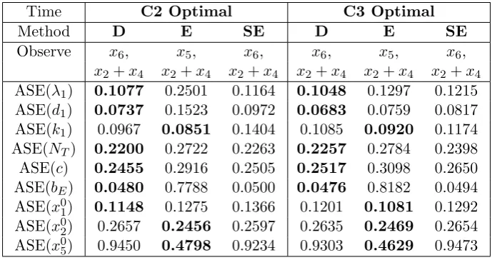
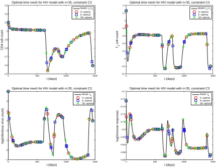
When choosingN = 2 observables and distributingn= 35 time points using constraint C2, the D-optimal cost function yields the lowest ASE for the parameters (λ1,d1,NT,c, bE, x01), but the

SE-optimals ASE are on the same order of magnitude (Table 5). Both the D- and SE-optimal cost functions selected the same observables, and they both were minimized by similar distributions of time points (Figure 1). The E-optimal design leads in the smallest ASE for (k1, x02, x05), with

an ASE(x0₅) that is half that of D-optimal and SE-optimal. E-optimal, however, trails D- and SE-optimal in the accuracy of an estimate forbE, with an ASE(bE) that is larger by one order of

magnitude. The large diﬀerence in ASE’s for these two parameters may be related to the observables selected by each design criterion: E-optimal design choosesx5 (the variable most closely related to

x0₅) as an observable when D- and SE-optimal choose x6 (whose right hand side containsbE). All

three also chosex2+x4. The distribution of time points selected under each optimal design criterion

(16)

Table 5: Approximate asymptotic standard errors calculated by asymptotic theory (25) using optimally spacedn= 35 time points under constraints C2 (left set of 3) and C3 (right set of 3) and optimally selectedN = 2 observables for parameters of interest ⃗θof the HIV model (27). Smallest ASE per parameter is highlighted using bold font.

Time C2 Optimal C3 Optimal

Method D E SE D E SE

Observe x6, x5, x6, x6, x5, x6,

x2+x4 x2+x4 x2+x4 x2+x4 x2+x4 x2+x4

ASE(λ1) 0.1077 0.2501 0.1164 0.1048 0.1297 0.1215

ASE(d1) 0.0737 0.1523 0.0972 0.0683 0.0759 0.0817

ASE(k1) 0.0967 0.0851 0.1404 0.1085 0.0920 0.1174

ASE(NT) 0.2200 0.2722 0.2263 0.2257 0.2784 0.2398

ASE(c) 0.2455 0.2916 0.2505 0.2517 0.3098 0.2650 ASE(bE) 0.0480 0.7788 0.0500 0.0476 0.8182 0.0494

ASE(x0₁) 0.1148 0.1275 0.1366 0.1201 0.1081 0.1292 ASE(x0₂) 0.2657 0.2456 0.2597 0.2635 0.2469 0.2654 ASE(x0

(17)

0 500 1000 1500 2.5

2.6 2.7 2.8 2.9 3 3.1 3.2 3.3

Optimal time mesh for HIV model with n=35, constraint C2

t (days)

CD4 cell count

Model: x₁+x₃ D−optimal E−optimal SE−optimal

0 500 1000 1500

−0.4 −0.2 0 0.2 0.4 0.6 0.8 1 1.2 1.4

t (days)

T2

cell count

Model: x₂+x₄ D−optimal E−optimal SE−optimal

0 500 1000 1500

−1 0 1 2 3 4 5 6

t (days)

log(Infectious virus count)

Model: x₅ D−optimal E−optimal SE−optimal

0 500 1000 1500

−0.88 −0.86 −0.84 −0.82 −0.8 −0.78 −0.76 −0.74 −0.72 −0.7

t (days)

log(Immune response)

Model: x₆ D−optimal E−optimal SE−optimal

Figure 1: Solution of (27) plotted using the observableslog(10x1₊₁₀x3_{) (upper left),}_log₍₁₀x2₊₁₀x4₎ (upper right),x5 (lower left), andx6 (lower right). Plotted on top of each curve are the D-optimal

(18)

0 500 1000 1500 2.5

2.6 2.7 2.8 2.9 3 3.1 3.2 3.3

t (days)

CD4 cell count

0 500 1000 1500

−0.4 −0.2 0 0.2 0.4 0.6 0.8 1 1.2 1.4

t (days)

T2

cell count

0 500 1000 1500

−1 0 1 2 3 4 5 6

t (days)

0 500 1000 1500

−0.88 −0.86 −0.84 −0.82 −0.8 −0.78 −0.76 −0.74 −0.72 −0.7

t (days)

(19)

ChoosingN = 2 observables and distributingn= 105 time points using constraint C2 leads to a diﬀerent pattern in which optimal design criterion is best for which parameter. For the more dense time point distribution, SE-optimal design is a much stronger candidate against D- and E-optimal (Table 6). It yields the lowest ASE’s for (λ1, NT, c, bE), while E-optimal is best for (k1, x01, x02, x05)

and D-optimal is best for (d1, bE). The D- and SE-optimal cost functions again choose the same

observables of x6 and x2+x4, so their ASE’s for all parameters are similar. In this scenario, the

E-optimal design has the largest percent reduction in ASE from those of D- and SE-optimal for the parametersx0₁ andx0₅. E-optimal also changed its selected observables tox1+x3 andx2+x4. The

distribution of time points for the D-optimal design criteria appear very close to uniform (Figure 3), and the distributions for E- and SE-optimal are clustered near local maxima, local minima, and other large changes in behavior of the observables; however, even slight diﬀerences between the distributions of the E- and SE-optimal costs functions are visible. Consider the graph of infectious virus count in Figure 3. There is a cluster of SE-optimal times betweent= 1100 andt= 1250, but no E-optimal times occur during that interval. Very soon after, between t= 1250 and t = 1400, there is a cluster of E-optimal times but no SE-optimal times. These clusters may indicate that either these periods in the patient’s treatment history are key to characterizing the parameters or that fewer time points may be adequate to obtain suﬃciently accurate parameter estimates.

The strength of SE-optimal design for large ndoes not hold for time grid constraint C3 (Table 6). E-optimal design provides the lowest ASE for the parameters (λ1, d1, k1, x01), D-optimal is best

for (NT, c, bE, x02, x05), and the ASE calculated using the SE-optimal designed experiment is often

the largest. The observables selected in this case are the same as then= 105, constraint C2 case. The optimal time point distributions determined under all three design criterion are near uniform (Figure 4). Small diﬀerences between the distributions may be observed when the functions have a slope of high magnitude, indicating that the distributions are not exactly uniform. As the time point optimization routine is started with a uniform time point distribution, this may indicate that when samples are taken at many times during an experiment, a uniform distribution is somewhat near optimal for model (27) or, more signiﬁcantly, that a uniform distribution is not an appropriate initial distribution to use to obtain the optimal time point distribution.

(20)

Table 6: Approximate asymptotic standard errors calculated by asymptotic theory (25) using optimally spaced n = 105 time points under constraints C2 (left set of 3) and C3 (right set of 3) and optimally selected N = 2 observables for parameters of interest ⃗θ of the HIV model (27). Smallest ASE per parameter is highlighted using bold font.

Time C2 Optimal C3 Optimal

Method D E SE D E SE

Observe x6, x1+x3, x6, x6, x1+x3, x6,

x2+x4 x2+x4 x2+x4 x2+x4 x2+x4 x2+x4

ASE(λ1) 0.0687 0.0618 0.0607 0.0674 0.0475 0.0729

ASE(d1) 0.0429 0.0541 0.0470 0.0441 0.0395 0.0475

ASE(k1) 0.0658 0.0360 0.0681 0.0629 0.0388 0.0739

ASE(NT) 0.1599 0.1437 0.1394 0.1192 0.1351 0.1423

ASE(c) 0.1785 0.1591 0.1551 0.1325 0.1500 0.1578

ASE(bE) 0.0281 0.4560 0.0281 0.0266 0.4637 0.0299

ASE(x0₁) 0.0810 0.0451 0.0793 0.0572 0.0490 0.0818 ASE(x0₂) 0.2537 0.2004 0.2296 0.1823 0.2244 0.2330 ASE(x0

(21)

0 500 1000 1500 2.5

2.6 2.7 2.8 2.9 3 3.1 3.2 3.3

t (days)

CD4 cell count

0 500 1000 1500

−0.4 −0.2 0 0.2 0.4 0.6 0.8 1 1.2 1.4

t (days)

T2

cell count

0 500 1000 1500

−1 0 1 2 3 4 5 6

t (days)

0 500 1000 1500

−0.88 −0.86 −0.84 −0.82 −0.8 −0.78 −0.76 −0.74 −0.72 −0.7

t (days)

(22)

0 500 1000 1500 2.5

2.6 2.7 2.8 2.9 3 3.1 3.2 3.3

t (days)

CD4 cell count

0 500 1000 1500

−0.4 −0.2 0 0.2 0.4 0.6 0.8 1 1.2 1.4

t (days)

T2

cell count

0 500 1000 1500

−1 0 1 2 3 4 5 6

t (days)

0 500 1000 1500

−0.88 −0.86 −0.84 −0.82 −0.8 −0.78 −0.76 −0.74 −0.72 −0.7

t (days)

(23)

6 Example 2: Zhu’s Calvin Cycle model

The second model we use as an example is characteristic of the large differential equation systems that often appear in industrial problems. In [19], Zhu et al., present an ODE model for the Calvin Cycle in fully grown spinach. The Calvin Cycle, part of the light-independent reactions in photosynthesis, plays an important role in plant carbon fixation, which leads to the growth of the plant. This model contains 165 parameters and initial conditions, 31 ODEs, and 7 concentration balance laws and involves 38 state variables (metabolite concentrations in different parts of the cell) as well as a calculation for photosynthetic CO2 uptake rate. The metabolites used in the model are

denoted by RuBP, PGA, DPGA, T3P, FBP, E4P, S7P, ATP, SBP, NADPH, HexP, PenP, NADHc, NADc, ADPc, ATPc, GLUc, KGc, ADP in photorespiration, ATP in photorespiration, GCEA, GCA, PGCA, GCAc, GOAc, SERc, GLYc, HPRc, GCEAc, T3Pc, FBPc, HexPc, F26BPc, UDPGc, UTPc, SUCP, SUCc, and PGAc, and the parameters are mainly initial conditions, maximum reaction velocities, and Michaelis-Menten constants for reaction substrates, products, activators, and inhibitors. The ‘c’ following some metabolite names indicates that the model compartment corresponds to the metabolite concentration in cytosol; compartment names lacking a ‘c’ are the metabolite in the chloroplast stroma. The full system of equations and parameter values may be found in the appendices of [19]. While the model has not been validated with data as completely as the family of HIV models discussed above, it is representative of the models used to describe plant enzyme kinetics and utilizes well-documented Michaelis-Menten enzyme kinetic model formulations [6].

In [5], sets of the optimal 3, 5, 10, and 15 metabolites are identiﬁed as the most useful to measure in an experiment in order to estimate a subset of 6 parameters, ⃗θa = [KM11, KM521,

KI523, KC, KM1221, KM1241]Twith true values ⃗θa0 = [0.0115, 0.0025, 0.00007, 0.0115, 0.15, 0.15]T,

and a subset of 18 parameters,⃗θc=[RuBP0, SBP0, KM11, KM13, KI13, KE4, KM9, KM131, KI135,

KE22, KM511, KM521, KI523, KC, KM1221, KM1241, V9, V58]Twith true values⃗θc0 = [2, 0.3, 0.0115,

0.02, 0.075, 0.05, 0.05, 0.05, 0.4, 0.058, 0.02, 0.0025, 0.00007, 0.0115, 0.15, 0.15, 0.3242, 0.0168]T. The simulation was set in the framework of an experiment run for 3000 seconds over which 11 samples are taken at evenly spaced times for the optimization of estimates for ⃗θa and 21 samples

for estimation of ⃗θc.

We use a similar set up for our simulations in order to judge the ability of the time and variable selections to minimize the asymptotic standard errors of both⃗θa and ⃗θc using N = 5 andN = 10

observables andn= 11 time points over the time intervalt∈[0,3000]. Each metabolite is assigned a variance of 5% of its initial value, and to reduce computation time, all metabolites that do not change in concentration over time (dx/dt = 0) are excluded from the search algorithm. As it is often possible to measure a particular metabolite’s concentration in plant tissue, we allow CN∗ to

be composed of 28 vectors in R1×40 that are composed of a one in the element corresponding to the position of the diﬀerential equation describing the dynamics of the metabolite in the vector of model ODEs and zero elsewhere.

(24)

Table 7: Top: Optimal 5 observables chosen by each optimal design criterion when estimating the parameters ⃗θa of the model in [19]. Bottom: Approximate asymptotic standard errors calculated

using asymptotic theory (25) for each parameter in ⃗θa using the optimal 5 observables with time

point constraints of uniform spacing, constraint C2, and constraint C3. Smallest ASE for each parameter per time point constraint is highlighted in bold font.

Method Observables

D-opt PGA, T3P, GOAc, SERc, F26BPc E-opt PGA, SERc, T3Pc, FBPc, F26BPc SE-opt PGA, SERc, T3Pc, FBPc, F26BPc

Time Uniform C2 Optimal C3 Optimal

Method D E SE D E SE D E SE

ASE(KM11) 0.0014 0.0356 0.0356 0.0015 0.0033 8.7e-4 5.8e-4 0.0018 0.0018

ASE(KM521) 4.1811 4.0086 4.0086 0.1324 0.1078 0.6805 0.0750 0.1349 0.0532

ASE(KI523) 0.1173 0.1125 0.1125 0.0037 0.0030 0.0191 0.0012 0.0038 0.0015

ASE(KC) 0.0012 0.0353 0.0353 0.0012 0.0033 0.0019 0.0011 0.0018 0.0018

ASE(KM1221) 0.2805 1.3065 1.3065 0.2742 0.4330 0.5798 0.1460 0.5127 0.5136

ASE(KM1241) 0.2508 1.1764 1.1764 0.2451 0.3874 0.5183 0.1305 0.4582 0.4592

The simplest scenario we test is the selection of the optimal N = 5 observables (metabolites) and n = 11 time points to use when estimating the six parameters in ⃗θa. For all three optimal

design methods, the optimal observables determined under the uniform grid were also determined to be optimal after the time point distribution is optimized under constraints C2 and C3. These observables are listed in the upper portion of Table 7. All three optimal design methods identify the observables PGA, SERc, and F26BPc, indicating that these three metabolites may be central to accurate estimates of the parameters inθ⃗a; moreover, the E-optimal and SE-optimal cost functions

selected the same set of ﬁve observables.

The similarity in results, however, does not continue through the selected time point distribu-tions. Under constraint C2 (Figure 5), the D-optimal distribution is loosely clustered about the center of the time interval, the E-optimal time points are clustered about t = 250 seconds, and SE-optimal chooses a small cluster of time points around the initial bump and allows a few samples after the function reaches a steady state. Using constraint C3 (Figure 6), all three optimal design criterion chose a majority of their sampling times before t = 600 and allow only a few sampling times after the system reaches a steady state. The optimization of time point distributions yields improved asymptotic standard errors from those of the uniform distribution - sometimes by an order of magnitude or more. For all three time point constraints, D-optimal yields the smallest ASE’s for the most number of parameters, and SE-optimal yields the smallest ASE’s for the second most number of parameters. Both optimal design criteria perform better with the C3 optimal times than the C2 optimal times. Therefore, in this simple case, using either the D- or SE-optimal design criterion with time point distribution constraint C3 would yield the best results.

The next scenario is the selection of the optimalN = 10 observables andn= 11 time points to use when estimating the six parameters in ⃗θa. For all three optimal design methods, the optimal

(25)

0 500 1000 1500 2000 2500 3000 0 0.1 0.2 0.3 0.4 0.5 0.6 0.7 0.8 0.9 1

Optimal time mesh for Zhu C3 model with n=11, constraint C2

t (seconds)

Carbon Uptake Rate A(t) (

µ

mol m

−2

s

−1)

Model: A D−optimal E−optimal SE−optimal

0 500 1000 1500 2000 2500 3000 0 0.1 0.2 0.3 0.4 0.5 0.6 0.7 0.8

t (seconds)

ATP

Model: ATP D−optimal E−optimal SE−optimal

0 500 1000 1500 2000 2500 3000 0 0.01 0.02 0.03 0.04 0.05 0.06 0.07 0.08 0.09 0.1

t (seconds)

Sucrose

Model: SUC D−optimal E−optimal SE−optimal

0 500 1000 1500 2000 2500 3000 0 0.5 1 1.5 2 2.5

t (seconds)

RuBP

Model: RuBP D−optimal E−optimal SE−optimal

Figure 5: Solutions of selected state variables in the Zhu model [19]. Plotted on top of each curve are the D-optimal (circle), E-optimal (square), and SE-optimal (x) n = 11 sampling times under constraintC2when sampling the optimal 5 observables to estimate⃗θa(Table 7). Top Left: Carbon

uptake rateA(t); Top Right: ATP; Bottom Left: SUCc; Bottom Right: RuBP.

upper portion of Table 8. Of the 28 possible observables, 20 were selected by at least one optimal design criterion, 8 of of which ( DPGA, T3P, E4P, S7P, ATP, GCA, SERc, T3Pc) were selected by two criteria and one, GOAc, was selected by all three. The effect of adding five observables does not have a large effect on the estimated ASE for the six parameters of interest. The ASE’s listed in Table 8 for theN = 10 observable case are on the same order as those in Table 7 for theN = 5 observable case for each time point constraint.

(26)

0 500 1000 1500 2000 2500 3000 0 0.1 0.2 0.3 0.4 0.5 0.6 0.7 0.8 0.9 1

t (seconds)

Carbon Uptake Rate A(t) (

µ

mol m

−2

s

−1)

Model: A D−optimal E−optimal SE−optimal

0 500 1000 1500 2000 2500 3000 0 0.1 0.2 0.3 0.4 0.5 0.6 0.7 0.8

t (seconds)

ATP

Model: ATP D−optimal E−optimal SE−optimal

0 500 1000 1500 2000 2500 3000 0 0.01 0.02 0.03 0.04 0.05 0.06 0.07 0.08 0.09 0.1

t (seconds)

Sucrose

Model: SUC D−optimal E−optimal SE−optimal

0 500 1000 1500 2000 2500 3000 0 0.5 1 1.5 2 2.5

t (seconds)

RuBP

Model: RuBP D−optimal E−optimal SE−optimal

Figure 6: Solutions of selected state variables in the Zhu model [19]. Plotted on top of each curve are the D-optimal (circle), E-optimal (square), and SE-optimal (x) n = 11 sampling times under constraint C3 when sampling the optimal 5 observables to estimate ⃗θa (Table 7). Top Left:

Carbon uptake rateA(t); Top Right: ATP; Bottom Left: SUCc; Bottom Right: RuBP.

errors from those of a uniform time distribution. For all three time point constraints, D-optimal yields the smallest ASE’s for the most number of parameters, and SE-optimal yields the smallest ASE’s for the second most number of parameters. Other than for the parameters it estimates best, SE-optimal is often the worst criterion. The time point distribution under constraint C2 allows smaller ASE’s for the N = 10 observable variables case. Therefore using the D-optimal design criterion with time point distribution constraint C2 would yield the best results.

The addition of ﬁve observables for ⃗θa does not greatly impact most of the calculated ASE’s.

For the time point constraints C2 and C3, all but one of the minimum ASE’s remain on the same order of magnitude, and some of the ASE’s increase when N = 10 observables are allowed from when N = 5 observables are allowed. This may indicate that for a small parameter set such as ⃗

θa, only a small amount of information is needed to obtain the best possible results; adding extra