University of Windsor University of Windsor
Scholarship at UWindsor
Scholarship at UWindsor
Electronic Theses and Dissertations Theses, Dissertations, and Major Papers
12-10-2018
Two Photon Processes within the Hyperfine Structure of
Two Photon Processes within the Hyperfine Structure of
Hydrogen
Hydrogen
Spencer Dylan Percy
University of Windsor
Follow this and additional works at: https://scholar.uwindsor.ca/etd
Recommended Citation Recommended Citation
Percy, Spencer Dylan, "Two Photon Processes within the Hyperfine Structure of Hydrogen" (2018). Electronic Theses and Dissertations. 7622.
https://scholar.uwindsor.ca/etd/7622
This online database contains the full-text of PhD dissertations and Masters’ theses of University of Windsor students from 1954 forward. These documents are made available for personal study and research purposes only, in accordance with the Canadian Copyright Act and the Creative Commons license—CC BY-NC-ND (Attribution, Non-Commercial, No Derivative Works). Under this license, works must always be attributed to the copyright holder (original author), cannot be used for any commercial purposes, and may not be altered. Any other use would require the permission of the copyright holder. Students may inquire about withdrawing their dissertation and/or thesis from this database. For additional inquiries, please contact the repository administrator via email
Two Photon Processes within the
Hyperfine Structure of Hydrogen
by
Spencer Percy
A Thesis
Submitted to the Faculty of Graduate Studies
through the Department of Physics in Partial Fulfillment
of the Requirements for the Degree of Master of Science at the
University of Windsor
Windsor, Ontario, Canada
c
Two Photon Processes in the Hyperfine Structure of
Hydrogen
by Spencer Percy APPROVED BY:
M. Monfared
Department of Mathematics and Statistics
E.H. Kim
Department of Physics
G.W.F. Drake, Advisor Department of Physics
Author’s Declaration of Originality
I hereby certify that I am the sole author of this thesis and that no part of this thesis has been published or submitted for publication.
I certify that, to the best of my knowledge, my thesis does not infringe upon anyone’s copyright nor violate any proprietary rights and that any ideas, techniques, quotations, or any other material from the work of other people included in my thesis, published or otherwise, are fully acknowledged in accordance with the standard referencing practices. Furthermore, to the extent that I have included copyrighted material that surpasses the bounds of fair dealing within the meaning of the Canada Copyright Act, I certify that I have obtained a written permission from the copyright owner(s) to include such material(s) in my thesis and have included copies of such copyright clearances to my appendix.
Abstract
The hyperfine levels for the ground state of hydrogen are normally connected by magnetic dipole transitions. However, for astrophysical applications, it may be that two-photon electric dipole processes are also important over cosmological distances. This thesis sets up a general mathematical formalism for the calculation of two-photon processes within the hyperfine structure of an atom with spin 1/2, and applies it to the ground state of hydrogen. Rates are calculated for both spontaneous emission and absorption of radiation. Due to an extraordinary degree of cancellation in the matrix elements, the rates turn out to be too small to have a significant impact on as-trophysical processes involving the absorption and emission of radiation. The results are nevertheless important in reducing the uncertainty due to possible contributions from these processes. Other two-photon processes involving Raman scattering are also considered and the relevant cross sections calculated. The calculations of the decay rate, absorption coefficient and Raman scattering cross section are extended to heavier hydrogenic ions as a function of the nuclear charge Z, using an approximate interpolation formula for the hyperfine splitting in the ground state. Results are pre-sented for the hydrogenlike ions from He+ to Pb81+. Modifications for the case of
Dedication
Acknowledgements
I’d like to thank my girlfriend Erica Dionisi for constantly helping me to suppress my imposter syndrome and always being in my corner. Daniel Venn for being the most consistent brot´eg´e I’ve ever had. Maha Sami for keeping the investigation into the identity of her husband alive. Aaron Bondy for his vast knowledge of Drew Dilkins. Kimberly Lefebvre for constantly listening to me complain. Joshuah Trocchi for being a friendly face while he squats in our office. Peipei Zhang for all the delicious moon cakes. A special thank you goes to the crew of The White Raven for saving the world from the Dread Captain Tiberius Flint
Contents
Author’s Declaration of Originality iii
Abstract iv
Dedication v
Acknowledgements vi
List of Figures ix
List of Tables x
1 Introduction 1
2 Hyperfine Splitting 5
2.1 Introduction . . . 5
2.2 Gross Structure . . . 6
2.3 Fine Structure Splitting . . . 7
2.4 Hyperfine Structure Splitting . . . 9
3 Sturmian Basis Sets 16 3.1 Sturmian Basis Sets . . . 16
4.1 Second-Order Perturbation Theory . . . 22
4.2 Single-Photon Transitions . . . 24
4.3 Two-Photon Transitions . . . 26
4.4 Applications to Hyperfine Transitions in Hydrogen . . . 30
4.5 Raman Scattering . . . 43
4.6 Z-scaling . . . 45
5 Conclusion 62 Appendix A 65 A.1 Hyperfine Angular Momentum Long Form . . . 65
A.2 Sturmian Basis Sets Calculation . . . 74
Bibliography 77
List of Figures
3.1 Variational calculation of the dipole polarizability of 1s hydrogen with
a two-term basis set . . . 20
3.2 Stability of the polarizability with size of basis set . . . 20
4.1 Time orderings of a two-photon process . . . 28
4.2 Calculation of the transition integrals |M−γγ(i→f)|2 . . . 36
4.3 Calculation of the decay rate A(ω) . . . 36
4.4 Calculation of the decay rate A . . . 38
4.5 Calculation of the absorption coefficient B11(ω) . . . 40
4.6 Calculation of the gain rate due to CMB radiation . . . 42
4.7 Calculation of the gain rate due to CMB radiation and a star . . . 42
4.8 Calculation of the gain rate due to a star . . . 43
4.9 Calculation of the Raman scattering cross section(ω) . . . 45
List of Tables
4.1 Hyperfine transition frequency for stable hydrogenlike isotopes with spin 1/2 nuclei. . . 48 4.2 Ground state hyperfine two-photon decay rate for hydrogenlike stable
isotopes with spin 1/2 nuclei. . . 49 4.3 Ground state hyperfine two-photon absorption coefficient for
hydro-genlike stable isotopes with spin 1/2 nuclei. . . 50 4.4 Raman scattering cross of the ground state hyperfine transition in
hy-drogenlike 2He3. . . 51 4.5 Raman scattering cross of the ground state hyperfine transition in
hy-drogenlike 6C13. . . 51 4.6 Raman scattering cross of the ground state hyperfine transition in
hy-drogenlike 7N15. . . 52 4.7 Raman scattering cross of the ground state hyperfine transition in
hy-drogenlike 14Si29. . . 52 4.8 Raman scattering cross of the ground state hyperfine transition in
hy-drogenlike 15P31. . . 53 4.9 Raman scattering cross of the ground state hyperfine transition in
hy-drogenlike 26Fe57. . . 53 4.10 Raman scattering cross of the ground state hyperfine transition in
drogenlike 39Y89. . . 54 4.12 Raman scattering cross of the ground state hyperfine transition in
hy-drogenlike 45Rh103. . . 55 4.13 Raman scattering cross of the ground state hyperfine transition in
hy-drogenlike 47Ag109. . . 55 4.14 Raman scattering cross of the ground state hyperfine transition in
hy-drogenlike 48Cd111. . . 56 4.15 Raman scattering cross of the ground state hyperfine transition in
hy-drogenlike 50Sn115. . . 56 4.16 Raman scattering cross of the ground state hyperfine transition in
hy-drogenlike 52Te125. . . 57 4.17 Raman scattering cross of the ground state hyperfine transition in
hy-drogenlike 54Xe129. . . 57 4.18 Raman scattering cross of the ground state hyperfine transition in
hy-drogenlike 69Tm169. . . 58 4.19 Raman scattering cross of the ground state hyperfine transition in
hy-drogenlike 70Yb171. . . 58 4.20 Raman scattering cross of the ground state hyperfine transition in
hy-drogenlike 74W183. . . 59 4.21 Raman scattering cross of the ground state hyperfine transition in
hy-drogenlike 76Os187. . . 59 4.22 Raman scattering cross of the ground state hyperfine transition in
hy-drogenlike 78Pt195. . . 60 4.23 Raman scattering cross of the ground state hyperfine transition in
drogenlike 81Tl203. . . 61 4.25 Raman scattering cross of the ground state hyperfine transition in
Chapter 1
Introduction
The purpose of this work is to take the well known hyperfine splitting in the ground state of hydrogen, and investigate two-photon transitions from the lower hyperfine level to the upper hyperfine level to see if the resulting absorption coefficient is a significant correction to astrophysical and cosmological phenomena. We are interested to see if the absorption coefficient is significant enough that it will provide a significant correction to light that is observed from distant stars. As the light travels through space it is absorbed by the hydrogen atoms through which it passes. The relevant frequencies are microwave frequencies between 0 and the transition frequency of the hyperfine splitting in the ground state of hydrogen being ν = 1,420,405,751.800 Hz. The 21 cmλ =c/ν wavelength for this transition wavelength has already made large contributions to our understanding of the universe, and we are interested to see if this particular transition can be a significant correction. In addition to this we will be investigating the role of this transition in Coherent Anti-Stokes Raman Scattering (CARS).
quanta, the sum of their energies is equal to the excitation energy, but each can be an arbitrary value” [1]. She also theorized that the reverse process was also possible being “the case that two light quanta, whose sum of frequencies is equal to the excitation frequency of the atom, work together to excite the atom” [1]. This concept was originally derived within the formulation of the Raman effect where a photon would interact with an atom and scatter with a different frequency. The main difference between these two processes is that two-photon absorption or decay deals with either a double annihilation or creation of two photons whereas the Raman effect deals with the annihilation then creation of photon or vice versa.
Through advancements in laser technology we know that these transitions are in-deed possible and have made large contributions to our understanding of the physical world. Quantum mechanically these transitions are dominant between states that would otherwise be forbidden. For example in hydrogen the 1s to 2s electric dipole transition is forbidden by parity and angular momentum selection rules, and thus cannot occur with a single photon process, two-photon processes are allowed for such a transition. Extensive work has been done on this process for hydrogen and helium-like atoms by Drake in “Spontaneous two-photon decay rates in hydrogen-like and helium-like ions” [2]. In this paper the decay rate increases in proportion to Z6, and so increases to (2.993±0.012)×1010 s−1 for Kr34+
Relativistic effects have also been calculated for this transition by Goldman and Drake in their paper “Relativistic two-photon decay rates of 2 s1/2 hydrogenic ions”
[3]. In their work all relativistic effects, retardation effects and all combinations of photon multipoles are taken into account. These effects are included because they make a significant contribution for all ions up to Z = 100
to the present investigation.
A group at John Hopkins University[5] has used two photon transitions and more specifically the two photon decay rate of the 2s state of hydrogen as a correction to recombination so that we can have a more complete picture of our universe closer to the Big Bang. Other two-photon transitions are also considered for this purpose such as higher energy s-states and higher energy d-states [6].
In addition to the work that has been done in two-photon processes, extensive work has been done on the topic of hyperfine splitting. In early astronomy, astronomers detected a very distinct hum coming from the center of our galaxy. The now famous 21 cm line in astrophysics was originally theorized by H. C. Van de Hulst in 1945. He was assigned as a student to find what spectral line could exist at radio frequency. He started with hydrogen naturally as it is the most abundant element in the universe, and that is as far as he needed to go. He found that the hyperfine levels of ground state hydrogen would produce radio waves of this frequency. With this new information astronomers were able to detect radio waves of this frequency and use it to find hydrogen throughout our galaxy. This all culminated in a paper published in 1954 by Van der Hulst and two of his colleagues where they proposed that our galaxy had a spiral structure [7].
Since the hyperfine splitting scales asZ3withZbeing the nuclear charge, there are several applications for hyperfine structure transitions in heavier ions. For sufficiently largeZ the hyperfine splitting will actually overtake the fine structure splitting of the ion [8].
Very recently the hyperfine splitting in the ground state of the heavy metal ion for Bismuth, Bi+82 has been studied extensively [9]. The experiment revealed that
tran-sitions in ground state hydrogenlike Bi+82and lithiumlike Bi+80. This seemed to have
solved the “hyperfine puzzle” and the theoretical magnetic moment was recalculated and found to be in closer agreement with experiment [10].
Two-photon processes are not simply limited to absorption and decay. In fact they are the basis for Raman and Rayleigh scattering processes. A photon is ab-sorbed and then a separate one is emitted and vice versa thus making a two-photon transition. Work has been done by Dalgarno and Sadeghpour in finding the Raman and Rayleigh scattering cross sections in both hydrogen and caesium [11]. They used an inhomogeneous differential equation method to calculate this cross section. We will be looking into their work for our own work on calculating the Raman Scattering cross section for the hyperfine levels of hydrogen.
Chapter 2
Hyperfine Splitting
In this chapter we will be going over the splitting of energy states that occur when considering fine structure and hyperfine structure. This is very important to the overall work as having a strong understanding of why this energy splitting occurs is crucial to dealing with transitions between these levels. We will briefly be going over the gross structure of the atom and the related quantum numbers. We will also be reviewing all of the quantum numbers that are involved in fine structure splitting as well as hyperfine structure splitting. We will show a derivation of how the spin-orbit coupling leads to fine structure splitting as well as how the spin-spin coupling of the electron with the spin of the nucleus leads to hyperfine splitting.
2.1
Introduction
the orbital angular momentum of the electron in units of~ and is responsible for the splitting of the quantum states of certain energy levels such as n = into 2s and 2p. The Azimuthal quantum number l is bound by n such that 0 ≤l ≤ n−1. Further separation of states occurs due to the magnetic quantum numberm orml which rep-resents the projection of the angular momentum onto the z-axis. The absolute value of this quantum number is bound by the orbital angular momentum of the state l
such that −l ≤ ml ≤ l. The final quantum number used to describe an electronic state is s, this number represents the spin angular momentum of the electron and is always 12. These quantum numbers are the ones most commonly used to describe a state of an atom and are perfectly acceptable for most general purposes; however, when high precision is involved there are more quantum numbers and interactions that are required.
2.2
Gross Structure
The gross structure of hydrogen is one of the most basic and fundamental atomic systems in quantum mechanics. Unlike most other many-electron systems, it is one that we can calculate analytically instead of making increasingly accurate approxi-mations. Although this is rather deceiving as an introduction to quantum mechanics it serves as the bedrock against which all quantum mechanical systems can be com-pared. In it’s most simplistic form it is the structure of the atom that is created by the interaction between the electron and its nucleus whose potential energy is given by(in SI units) [8]
V(r) = −Ze
2
4π0r
(2.1)
equation
H0Ψ =EΨ (2.2)
with
H0 =− ~ 2
2m∇
2− Ze2
4π0r
(2.3)
therefore
−
~2
2m ∇
2+V(r)
Ψ =EΨ (2.4)
where the energies are given by
En =−
e2Z2
2a0n2
(2.5)
and a0 =~2/mc2 is the Bhor radius.
2.3
Fine Structure Splitting
The coupling between an electron spin and it’s orbit gives rise to fine structure split-ting and the total angular momentum quantum number represented by J where
J=L+S. (2.6)
is the total angular momentum including spin. These different values for the total angular momenta give rise to different energy levels within a state of a given principal quantum number n. An example of this is the splitting of the 2p state. With the given values ofl = 1 ands= 12, this spin-orbit coupling gives rise to the fine structure states of J = 12 and J = 32. To calculate this energy splitting we treat the spin-orbit coupling as a small perturbation to the Hamiltonian, where the total Hamiltonian is [12]
with
ξ= ~
2m2 0c2
D1
r dV
dr
E
(2.8)
The transformation from the ml, ms representation to the j, mj representation in Dirac notation is defined by
|nljmji=
X
mlms
|nlmlmsi hlsmlms|lsjmji (2.9)
wherehlsmlms|lsjmjiis a Clebsch-Gordan coefficient [13]. The expectation value for the first order correction to the energy is [12]
∆E1 =hnljmj|ξl·s|nljmji (2.10)
We use the fact that|nljmjiis an eigenfunction ofj2,l2,s2, andjz to avoid calculating the Clebsch-Gordan coefficients. Using the fact that
j2 = (l+s)·(l+s) =l2+s2+ 2l·s (2.11)
we can write
l·s= 1 2(j
2−
l2−s2) (2.12)
Which gives the result
∆E1 =
ξ
2hnljmj|j
2−
l2−s2|nljmji
= ξ
This leads to an energy splitting between the 2p1
2 state and the 2p 3
2 in atomic units
by use of the expression
ωp3 2−p
1 2 =
α2Z4
4n3 = 1.665×10
−6 (2.13)
in atomic units with Z = 1. This is several orders of magnitude smaller than the transition energy between the ground state and first excited state, which is in atomic units
1 2 −
1 8 =
3
8 (2.14)
.
2.4
Hyperfine Structure Splitting
In addition to the fine structure spitting there is a further level of splitting known as hyperfine splitting. This energy level splitting is again caused by the coupling of two different angular momenta. However, in this case it is the coupling of the total angular momentum of the electronJ and the spin angular momentum of the nucleus
I. In the s-states of hydrogen this splitting is particularly prominent. This is due to the fact the wave equation of the electron in the s-state is non-zero at radius zero. This is the reason for the hyperfine energy splitting to be as large as it is in the s-states. The quantum number that we use to denote this hyperfine-energy levels is
F where
F=J+I, (2.15)
takes the form [14]
H =H0+H1 (2.16)
where
H1 =−µI·Bel (2.17)
and it is assumed that the zeroth order Hamiltonian H0 contains the terms that
allow us to evaluate the separate energy levels corresponding to eachJ. We make the assumption that we are only dealing with an isolated manifold of the hyperfine states labeled byJ, and that hyperfine splitting is small compared to fine structure splitting. We will refer to this approximation as theIJ coupling approximation, similar to LS
coupling approximation in fine structure. Using this we can rewrite the point nuclear magnetic moment µI as [14]
µI =
µI
I I (2.18)
with µI being the value of the nuclear magnetic moment. We can also note that
Bel ∝ J with the assumption that the operator operates in the space of electron coordinates only. This allows us to rewrite our Hamiltonian as
H1 =AI·J (2.19)
with A being determined through measurements of experimental transition frequen-cies.
field operator as [14]
Bel =
µ0
4π
(−ev)×(−r)
r3 −
µ0
4π
1
r3
µs−
3(µs·r)r
r2
(2.20)
Then using µs = −2µBs and −er×v = −2µbl with µB being the Bohr magneton, we rewrite the magnetic field as
Bel =−2
µ
4π µB
r3
l−s+ 3(s·r)r
r2
, l 6= 0 (2.21)
and thus rewrite the perturbed part of the Hamiltonian as
H1 =
µ0
4π
2µB
µI
I
I·N
r3 (2.22)
with
N=l−s+ 3(s·r)r
r2 . (2.23)
We create zeroth-order wave equations |γIjF Mfi which are linear combinations of |γIMIjmjiwhere
F=I+j (2.24)
with F being the new total angular momentum. According to perturbation theory we write our corrected Hamiltonian H , wave equation Ψ, and energy E in the form
H =H0+λH1
Ψ = Ψ0+λΨ1+λ2Ψ2 +...
E =E0 +λE1 +λ2E2+...
(2.25)
where λ is a constant. We use these new perturbation expansions to solve the Schr¨odinger equation such that
then, retaining terms up to the first order
(H0+λH1)(Ψ0+λΨ1) = (E0+λE1)(Ψ0+λΨ1) (2.27)
and
H0Ψ0+λH1Ψ0+λH0Ψ1+λ2H1Ψ1 =E0Ψ0+λE1Ψ0+λE0Ψ1+λ2E1Ψ1 (2.28)
using the fact that
H0Ψ0−E0Ψ0 = 0
H1Ψ1−E1Ψ1 = 0
(2.29)
we then have
λH1Ψ0+λH0Ψ1 =λE1Ψ0+λE0Ψ1 (2.30)
Rearranging, removing the common factor ofλ, and acting from the left by Ψ0
Ψ†0H1Ψ0+ Ψ
†
0H0Ψ1 = Ψ
†
0E1Ψ0+ Ψ
†
0E0Ψ1 (2.31)
which after integration reduces to
E1 =hΨ0|H1|Ψ0i (2.32)
which allows us to define our energy due to hyperfine structure as
∆E =hγIjF Mf|H1|γIjF Mfi. (2.33)
matrix elements that are diagonal in j. This changes our Hamiltonian to
H1 =
µ0
4π
2µB
µI
I
N·j
j(j+ 1)
I·j
r3 . (2.34)
Then
∆E =
µ0
4π
2µB
µI
I
N·j
j(j+ 1)r3
1
2{F(F + 1)−j(j + 1)−I(I+ 1)} (2.35)
=aj{F(F + 1)−j(j+ 1)−I(I+ 1)} (2.36)
where
aj =
µ0
4π
2µB
µI
I
N·j
j(j+ 1)r3
, l 6= 0 (2.37)
we have,
N·j= (l−s)(l+s) + 3(s·r)r
r2 ·(l+s)
=l2−s2+ 3(s·r)(r·l)/r2+ 3(s·r)(r·s)/r2
(2.38)
and using the fact that ~l=r×p implies that r·l= 0 and due to the triangle rule of angular momentum algebra
s2+ 3(s·r)2/r2 = 0 (2.39)
which reduces our equation to
N·j=l2 (2.40)
and, taking expectation values leads to
aj =
µ0
4π
2µB
µI I 1 r3
l(l+ 1)
j(j + 1), l 6= 0 (2.41)
s state (l = 0) which is the particular case being studied. The fact that an electron in an s state has a nonzero probability density at the origin
|ψ(0)|2 6= 0 (2.42)
gives rise to an interaction between the nuclear moment and the intrinsic spin mag-netic moment of the electron in an s-state. This is known as the Fermi contact interaction, and it has the form
H1 =asI·s =asI·J
(2.43)
since for the s electron l = 0 =⇒ s=J, with
as=
µ0
4π
2µB
µI
I
(8π/3)|ψ(0)|2, l= 0. (2.44)
A relativistic treatment is not necessary for this derivation. We take semiclassical considerations, such as the fact that for an electron in an s-state, there is a spherically symmetric distribution of spin magnetism which does not vanish at the origin. The spin magnetic moment per unit volume at the origin is [14]
P0 =µs|ψ(0)|2. (2.45)
where [15]
µs=
q~
2mgss (2.46)
where s is the spin of the test charge, q~
uniform magnetization P0,
B= (2µ0/3)P0 = (2µ0/3)µs|ψ(0)|2 (2.47)
This implies that the magnetic interaction of a point nuclear magnetic moment with this field is
H =−(2µ0/3)µI·µs|ψ(0)|
2
(2.48)
Using this we can calculate as for the case for hydrogen in an s-state,
|ψ(0)|2 = Z
3
πa3 0n3
(2.49)
therefore
as =
µ0
4π
2µB
µI
I
8 3
Z3
a3 0n3
, l = 0 (2.50)
Chapter 3
Sturmian Basis Sets
Before we begin going into two-photon processes we must first develop a few com-putational techniques. When dealing with a two-photon process, the transition from initial to final state is connected by an intermediate state. This intermediate state is actually a summation over all possible bound states as well as an integration over the continuum. This is computationally very intensive and difficult to deal with. Instead we will be developing a technique that uses a discrete set of variational pseudostates to represent the entire spectrum of hydrogen. As a demonstration of this technique we will be showing how the entire spectrum of hydrogen can be represented by two pseudostates for the calculation of the polarizability. The particular calculation we will be doing to represent this is a calculation of the static polarizability of hydro-gen. This is a known value that can be calculated analytically and so is a strong demonstration of the power of the technique.
3.1
Sturmian Basis Sets
according to
∆E = 1 2αdF
2 (3.1)
Where F is the field strength and αd is the polarizability. In this chapter we develop computational methods for this as a test case that will be applied later to two-photon processes. The dipole polarizability is defined by the second-order perturbation ex-pression [16]
αd≡ −E(2) =−
Z ∞
X
n=1
|hnp|eF rcosθ|1si|2 En−E1s
(3.2)
where the summation over n includes an integration over the continuous part of the spectrum, andE(2) is the second-order perturbation energy due to the external field.
In this particular example the ground state is the 1s state and the intermediate virtual states are represented by the p-states connected by electric dipole transitions. The expression as it stands involves a summation over the entire spectrum of p-states and then an integration over the continuum. This however is difficult to do in practice. We instead use the pseudostate method along with the variational method to sum over a discrete variational basis set with no integration over the continuum. The first set of using this method is generating the pseudostates. To do this we first define what sort of basis set we wish to use. Since the field-free Hamiltonian is spherically symmetric, we use spherical coordinates as this makes the resulting integrals rather elegant to evaluate analytically. Every state is expanded in the basis set of functions
rne−αrYlm(θ, φ) [17]
Ψ(r) = N
X
n=1
cnrne−αrYlm(θ, φ) =
X
n
cnχn (3.3)
χn =rne−αrYlm(θ, φ) (3.4)
same functional form as hydrogenic wave functions. In addition, all integrals can be evaluated analytically using
Z ∞
0
rne−αrdr= n!
αn+1. (3.5)
First we must create out basis set by forming linear combinations. We do this by generating an overlap matrix whose elements are [17].
χn(r) =rne−αrYlm(θ, φ) (3.6)
Omn =hχm|χni (3.7)
The way this matrix is orthogonalized is by the Jacobi method,(see Appendix) which works in this case because our matrix is symmetric.
3.2
Dipole Polarizability
We now apply the sets of pseudostates to the calculation of the polarizability of ground-state hydrogen. We consider a hydrogen atom in the ground state placed in a static electric field of strength F pointing in the z direction. This gives rise to the perturbation V = eF rcosθ. In the case of hydrogen, the first order perturbation equation can be solved analytically as further discussed below. However as a test of the pseudostate method, we will use it instead to calculate the second-order correction to the energy. This is useful because we can use this very simple example to test that the method works and can then be applied to much more complex examples. The
correction to the energy.
E(2) = N
X
n=1
|hnp|eF rcosθ|1si|
2
En−E1s
(3.8)
Taking this with the definition of the dipole polarizability
αd ≡ −E(2) (3.9)
which for the case of the ground state of hydrogen becomes αd= 92a30 wherea0 is the
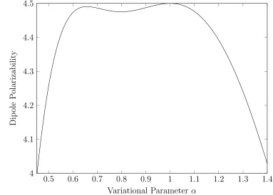
Bohr radius. There are several things worth mentioning about this technique. The first concerns the variational parameterα. If we were to take our expression evaluated with a small basis set and plot is as a function of α we can see that there is a rather significant variation as shown in Fig.3.1. However we can very plainly see an absolute maximum located atα= 1 [16]. We can also see that the true value ofαdis an upper bound to our function and no matter how large we expand our basis set that ceiling of the true value of 4.5a30 is never exceeded. Note that all the contributions to Eq. (3.8) are positive.
Figure 3.1: Variational calculation of the dipole polarizability of 1s hydrogen with a two-term basis set
0.5 0.6 0.7 0.8 0.9 1 1.1 1.2 1.3 1.4 4
4.1 4.2 4.3 4.4 4.5
Variational Parameter α
Dip
ole
P
olarizabilit
y
Figure 3.2: Stability of the polarizability with size of basis set
0 0.2 0.4 0.6 0.8 1 1.2 1.4 1.6 1.8 2 0
1 2 3 4
Variational Parameter α
Dip
ole
P
olarizabilit
y
N = 2
N = 3
N = 4
For our purposes however we can arrive at the exact result of 4.5a3
0 using only a
two dimensional basis set with matrix elements and energies of [16]
ψ1 =re−r−
r
8 45r
2e−r
E1 =−
1
10 a.u.
ψ2 =
√
8re−r−2
√
2 3 r
2e−r
E2 =
1 2 a.u.
(3.10)
Chapter 4
Two Photon Processes
In this chapter we will begin reviewing the theories that are involved in a two-photon process. Two-photon processes come about through second-order perturbation theory so a brief description of it will allow for a greater understanding of the topic as a whole. We will be looking at how photons interact with matter to develop the operator we will be using in this study. From there we will be reviewing how time-orderings of the two photons is involved as well as how the basic theory works overall. This chapter will also discuss our results and derivation of the two-photon decay rate, how it relates to its two-photon Einstein B absorption coefficient and the results of it being applied to astrophysics. In addition to this we will be going over how it can be applied to Raman scattering as well as a brief discussion of how Raman and Rayleigh scattering differ from each other and other two-photon processes. Finally we will be presenting our results of all of these calculated values as they are scaled up through heavier hydrogenlike ions.
4.1
Second-Order Perturbation Theory
[16]
H =H0+λH1 (4.1)
where H0 is our unperturbed Hamiltonian which can be solved for analytically, and
V is our perturbation which is controlled by the parameter λ. We then expand our wave equations and energies in terms of our scale factor λ
Ψ = Ψ0+λΨ1+λ2Ψ2
E =E0+λE1+λ2E2
(4.2)
First-order perturbation was derived in a previous section so we will only focus on second-order perturbation here. Solving for the second order correction to the energy we have
E2 =
1
hΨ0|Ψ0i
[2hΨ0|V |Ψ1i+ 2hΨ0|H0−E0|Ψ2i+hΨ1|H0−E0|Ψ1i] (4.3)
This is formed from terms withλ2. E2 is stable with respect to variations of Ψ2, the
second-order perturbation equation is
(H0−E0)|Ψ2i+ (V −E1)|Ψ1i=E2|Ψ0i (4.4)
then it follows that
E2 =
hΨ0|V −E1|Ψ1i
hΨ0|Ψ0i
(4.5)
and using the definition of Ψ1 if it satisfies the first-order perturbation equation
|Ψ1i=
−(V −E1)|Ψ0i
H0−E0
(4.6)
we then multiply by unity
1 =
Z ∞
X
n=1
to get our first-order perturbation to the wave equation as
|Ψ1i=
Z ∞
X
n=1
|Ψni hΨn| −(V −E1)|Ψ0i
E0n−E0
(4.8)
which we then substitute into our second-order perturbation to the energy to give
E2 =
Z ∞
X
n=1
hΨ0|V −E1|Ψni hΨn| −(V −E1)|Ψ0i
E0n−E0
(4.9)
For the particular case of solving the dipole polarizability for the s-state we use the fact that E1 = 0 for the operator used is V = F rcosθ. As detailed in previous
sections we use a discrete basis set to represent the intermediate states, rather than summing over the entire spectrum and integrating over the continuum. The purpose of this derivation will be made obvious in the following sections, as the equation for the second-order perturbation is extremely similar to the matrix elements of a two-photon transition.
4.2
Single-Photon Transitions
In this section we will detail the derivation of the form of the interaction operator that we will be using in our two-photon transition. We first start from the definition of the Hamiltonian
H = p
2
2m +V (4.10)
through which we make the transformation to the canonical momentum
~
p→~p− e c
~
the Hamiltonian then becomes
H = (~p− e cA~)
2
2m +V
= p
2
2m − e
2mc~p·A~+ e
2mcA~·~p+ e2
2mc2A~ 2+V
(4.12)
where
~
A=A0eeˆ i~k·~r−iωt (4.13)
is the vector potential for a plane wave. Using the definition of a plane wave
~k
=ω/c (4.14)
being of order α= 1/c in atomic units and
~k·eˆ= 0 (4.15)
for a transverse wave, we expand the Hamiltonian as
H = p
2
2m −
2eA0
2mc~p·ˆe[1−i~k·~r+· · ·]e −iωt
(4.16)
Keeping only the first order term and using the fact that ∇ ·A = 0 for a transverse wave we have
H1 =−
eA0
2mc2~p·eˆ (4.17)
We then calculate the transition matrix elements
and use the commutator relation to get the operator into length form where
m
~
hΨi|[H , ~r·eˆ]|Ψfi=
m
~
(Ei−Ef)hΨi|~r·eˆ|Ψfi (4.19)
This is the form of the interaction operator used in the next section for the two-photon transitions that are being studied. From this we can also show how energy is conserved. Using definitions for the time dependent portion of the wave equations where
Ψi =e−iEit/~ (4.20)
and
Ψf =e−iEft/~ (4.21)
This leads to the time integral
Z ∞
0
(e−iEit/~)∗e−iωte−iEft/~dt = 2πδ
Ei
~ −ω−
Ef
~
(4.22)
which leads to the conservation of energy relation
ω = (Ei−Ef)~ (4.23)
4.3
Two-Photon Transitions
The most probable atomic transitions involve emission or absorption of a single pho-ton, where an atom starts in an initial state and then either absorbs or emits a single photon to go into either a higher or lower state respectively. We can represent this transition in bra-ket notation with the initial state|iibeing operated on by the dipole operator ˆe·~r to arrive at our final state |fi. The dipole matrix element is then
hf|ˆe·~r|ii (4.24)
The construction of a two-photon transition is very similar. The major difference being that there is an intermediate virtual state in between the initial and final states. Starting with the initial state|ii, operated on by ˆ·~rto go to an intermediate virtual state hn|. A second transition is then done by operating on the intermediate virtual state with ˆ·~r to excite to the final state hf|.
hf|eˆ·~r|ni hn|ˆe·~r|ii (4.25)
The energies of the two photons do not have to be identical. The only constraint on them is that the sum of their energies must equal the transition energy from the initial state to the final state, due to conservation of energy. This brings up a unique problem in that the photons are not indistinguishable from each other. So the order in which the photons interact with the atom matter, and we must consider the three possible time-orderings that can occur.
Figure 4.1: Time orderings of a two-photon process
can occur. it is assumed that the process happens instantly. The first time ordering shows the atom absorbing the first photon ˆe1, jumping to an intermediate state,
absorbing the second photon ˆe2 and jumping to the final state. The second time
ordering shows the same process except the order of the photons is reversed. The final time ordering shows both of the photons being absorbed simultaneously, this is a second order term and is therefore far less probable. The equation now changes to account for the specific order that the two photons are absorbed so that we average over the two time-orderings.
|hf|ˆe2·~r|ni hn|eˆ1·~r|ii+hf|ˆe1·~r|ni hn|eˆ2·~r|ii| 2
(4.26)
demonstration. Using the previously built equations for two-photon processes along with the summation over pseudostates, from the previous chapter, our expression for the matrix elements of this transition is proportional to.
X n
h2s|z|ni hn|z|1si En−E0+ω1
+h2s|z|ni hn|z|1si
En−E0+ω2
2 (4.27)
When considering the exchange of angular momentum going from a 1s state where
l = 0 to a 2swherel = 0 the triangular rule tells us that the total angular momentum exchanged is 0. This is relevant due to the fact that each photon carries with it one unit of angular momentum. For this to occur the two photons are antiparallel thus the total angular momentum exchanged sum to zero. From this we calculate a full decay rate
A(ν1)dν1 =
1024π6e4
~2c4 ν
3 1ν
3
2|(ˆe1·eˆ2)| 2 X n
h2s|z|ni hn|z|1si En−E0+ν1
+ h2s|z|ni hn|z|1si
En−E0+ν2
2 (4.28) with the total decay rate given by
A= 1 2
Z ν
0
A(ν1)dν1 (4.29)
where the factor of 12 is introduced because only unique pairs of photons are to be counted. Observing the terms in this equations we see that the decay rate will be greatest when ω1 = ω2 when the polarization of the polarization vectors are parallel
4.4
Applications to Hyperfine Transitions in
Hy-drogen
The hyperfine levels in ground-state hydrogen are represented by the eigenvectors
|1slsJ IF Mfi (4.30)
with s and l representing the electrons spin and orbital angular momentum. These two angular momenta couple together to give the total angular momentum J which is coupled with the spin of the nucleus I to give the quantum number for hyperfine levels F. With Mf being the projection of F onto the z-axis. The hyperfine levels of the ground state are separated into the two levels F = 0 and F = 1. Since this is a transition between two s states, single-photon electric-dipole transitions are forbidden due to angular momentum and parity selection rules. Therefore two-photon processes are required. We will specifically be calculating the decay rate and absorption coefficient due to this process and will see if it is a potentially significant correction to astrophysical processes on cosmological distance scales. In addition to this, we will also be calculating cross sections for Raman scattering. For either of these processes we must first calculate the matrix elements using the equation
M−γγ(ˆe
i →eˆf) =
X
n
hf|eˆ2·~r|ni hn|ˆe1·~r|ii
ωni+ω1
+hf|ˆe1·~r|ni hn|eˆ2·~r|ii
ωni+ω2
(4.31)
with both time-orderings of the photons being considered and all polarizations ˆe of the two photons being accounted for by the dipole operator ˆe·~r where
ˆ
r0 =z
r±=∓
1
√
2(x±iy)
(4.33)
e0 =ez
e±=∓
1
√
2(ex±iey)
(4.34)
and by conservation of energy
~ω1+~ω2 =Ei−Ef (4.35)
Summing this expression over all polarizations gives
M−γγ(i→f) =
1
X
µ1=−1
1
X
µ2=−1
X
n
(−1)µ2(−1)µ1hf|eµ2r−µ2|ni hn|eµ1r−µ1|ii ωni+ω1
+(−1)µ1(−1)µ2hf|eµ1r−µ1|ni hn|eµ2r−µ2|ii ωni+ω2
.
(4.36)
We may now include all the relevant quantum numbers for these transitions with the corresponding eigenvectors given by
|1slsJ IF Mfi (4.37)
for the initial state
npl0s0J0I0F0Mf0
(4.38)
as the intermediate state, and
as the final state. For the current purposes the only two quantum numbers that matter are the hyperfine splitting quantum number F and its projection Mf. The rest will be written together as γ. We must also sum over all possible magnetic quantum numbers for the final states and over the intermediate states with Mf00=−1,0,1 and
Mf0 =−1,0,1. Rewriting the transition equations gives us
M−γγ(F →F00) =
1
X
Mf00=−1 1
X
Mf0=−1 1
X
µ1=−1
1
X
µ2=−1
X
n
(−1)µ2(−1)µ1hγ
00F00M00
F|eµ2r−µ2|γ 0F0M0
Fi hγ0F0MF0 |eµ1r−µ1|γF MFi ωn0+ω1
+(−1)µ1(−1)µ2hγ
00F00M00
F|eµ1r−µ1|γ 0F0M0
Fi hγ
0F0M0
F|eµ2r−µ2|γF MFi ωn0+ω2
.
(4.40)
To evaluate these matrix elements we first strip away the dependence on the mag-netic quantum numbers by using the Wigner-Eckart theorem to calculate the reduced matrix element [20]
(γ0j0m0Tqk
γjm) = (−1)j
−m
j0 k j
−m0 q m
(γ 0 j0 Tk
γj) (4.41)
or in this case
(γ0F0Mf0|r−µ|γF MF) = (−1)F−MF
F0 1 F
−MF0 −µ MF
(γ
0
F0||r||γF) (4.42)
This changes our equation to
M−γγ(F →F00) =−
r
1 18
X
n (e2×e1)
(γ00F00||r||γ0F0)(γ0F0||r||γF)
ωn0+ω1
+(e1×e2)
(γ00F00||r||γ0F0)(γ0F0||r||γF)
ωn0+ω2
.
Using the fact that
(e1×e2) = −(e2×e1) (4.44)
and that we must now strip away the dependence on the coupling of the total angular momentum with the spin of the nucleus we rewrite our equation as
M−γγ(F →F00
) =−
r
1
18(e2×e1)
X
n
3/2
X
J0=1/2
(γ00J00I00F00||r||γ0J0I0F0)(γ0J0I0F0||r||γJ IF)
ωn0+ω1
−(γ
00J00I00F00||r||γ0J0I0F0)(γ0J0I0F0||r||γJ IF) ωn0 +ω2
.
(4.45)
It is significant that as in the case of triplet helium decay [4] where one unit of angular momentum is exchanged in a two-photon process, the matrix element is proportional to the cross product of the polarization vectors, leading to a minus sign between the two terms. We now use the definition of a 6j symbol for two coupled angular momenta [21]
(γ0j10j2J0||T(k)||γj1j2J)
= (−1)j01+j2+J+k[(2J+ 1)(2J0+ 1)]12
j10 J0 j2
J j1 k
(γ0j10||T(k)||γj1)
(4.46)
reduced matrix element
M−γγ(i→f) = 1
9(e2×e1)
X
n (1s||r||np)(np||r||1s)
ωn3 2
0+ω1
+ (1s||r||np)(np||r||1s)
ωn1 2
0+ω2
−(1s||r||np)(np||r||1s) ωn1
2
0+ω1
− (1s||r||np)(np||r||1s) ωn3
2
0+ω2
(4.47)
From here we can use the Wigner-Eckart theorem for 3j symbols to calculate the reduced matrix element
(γ0j0||T(k)||γj) = (γ
0j0m0|T(kq)|γjm)
(−1)j0−m0
j0 k j
−m0 q m
(4.48)
For this we use the z operator and ml = 0 for the magnetic quantum numbers as it is convenient to calculate analytically. This changes the resulting equation to
M−γγ(i→f) =−1
3(e2×e1)
X
n
h1s|z|npi hnp|z|1si
1
ωp3 20
+ω1
+ 1
ωp1 20
+ω2
− 1
ωp1 20
+ω1
− 1
ωp3 20
+ω2
(4.49)
To display explicitly the difference between the J0 = 12 and J0 = 32 p-states, we find a common denominator. We also take the approximation that the fine structure splitting is relatively small compared to the other energy terms
1
ωp3 2
0+ω
− 1
ωp1 2
0+ω
= ω3/2−1/2
ω2
p0+ 2ωp0ω+ω2
(4.50)
whereω3/2−1/2 =ωp3 20
−ωp1 20
the fine structure energy shift [22]
W1 =−
α2Z4
2n3
1
j+ 12 − 3 4n
(4.51)
and evaluate the difference between two states where j = 32 and j = 12, we have the expression
ωp3 2−p
1 2 =
α2Z4
4n3 (4.52)
Taking this into account and also considering the fact that the matrix elements are real numbers, the equation becomes
M−γγ(i→f) = −1
3(e2×e1)
X
n
hnp|z|1si2
ω3/2−1/2
ω2
p0+ 2ωp0ω1+ω21
− ω3/2−1/2 ω2
p0+ 2ωp0ω2+ω22
(4.53)
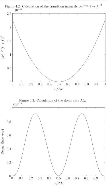
which gives the final form for the matrix elements that will be used in the calculation of the decay rate, the absorption coefficient, and the Raman scattering cross section. We calculate this using a variational intermediate basis set with results being in Fig.4.2. As can be seen in the graph, the transition integral becomes zero when the frequencies of the two photons are equal. We will first apply this to the calculation of the decay rate using the equation [4]
A(ν1) =
1024π6e4
h2c6 ν 3 1ν
3 2
M−γγ(i→f)
2
(4.54)
which we change over to a form better suited for the program that we use, that form being as a relation of angular frequency ω
A(ω1) =
16e4
c6 ω 3 1ω
3 2
M−γγ(i→f)
2
(4.55)
inte-Figure 4.2: Calculation of the transition integrals |M−γγ(i→f)|2
0 0.1 0.2 0.3 0.4 0.5 0.6 0.7 0.8 0.9 1 0
0.5 1 1.5 2 2.5
·10−24
ω/∆E
|M
−
γ
γ (
i
→
f
)
|
2
Figure 4.3: Calculation of the decay rate A(ω)
0 0.1 0.2 0.3 0.4 0.5 0.6 0.7 0.8 0.9 1 0
0.2 0.4 0.6 0.8 1
·10−78
ω/∆E
Deca
y
Rate
A(
ω
grated over all possible values for ω to arrive at the full decay rate. Due to the fact that
ω2 = ∆EF=0→F=1−ω1 (4.56)
the double integration overω1 andω2 reduces to a single integral overω1. In addition
to this, due to the symmetric distribution about the mid pointω1 =ω2, we need only
account for half of the total integral. This leaves us with the integral.
A=
Z ∆EF=0→F=1
0
A(ω1)dω1 (4.57)
which we integrate using the trapezoidal rule. This leads us to the result of
A = 1.97(3)×10−69s−1 (4.58)
which is an extremely small value. This value however is several orders of magnitude larger than the value calculated by V. P. Demidov. He approximated the value of this transition to be 7.6×10−73s−1 [23]. The stability of excited hyperfine ground
state hydrogen leads to a lifetime of several million years in the single magnetic photon case [19], but in this case it is several orders of magnitude greater than that. The stability of the calculation can be seen in Fig.4.4 where it can be seen that the expression converges to an upper bound of the true value as the basis set is enlarged. For the polarizability we can represent the entire spectrum of hydrogen with a two-dimensional basis set. However in this case we need a much larger basis set due to the fine structure energy splitting being dependent on the basis set size.
Figure 4.4: Calculation of the decay rate A
2 4 6 8 10 12 14 16 18
2 2.2 2.4 2.6 2.8
·10−69
Dimension of Basis set
Deca
y
Rate
A
start from the loss rate D and gain rate N of the system [25].
D=A+B22ρ1ρ2+B21ρ2+B12ρ1
N =B11ρ1ρ2
ρi =
8πh c3
(ehνi/kT −1)ν3
i
(4.59)
where A is the spontaneous decay rate, B22 is the doubly stimulated decay rate, B12
and B21 are the singly stimulated decay rates for the two separate photon orders and
coefficient in terms of the decay rate
N
D =
A ρ1ρ2
+B22+
B21
ρ1
+B12
ρ2
−1
B11
=e−∆E/kT
g2
g1
A ρ1ρ2
+B22+
B21
ρ1
+ B12
ρ2 = c3 8πh 2 A ν3
1ν23
+B22+
c3 8πh B21 ν3 1 + c3 8πh B12 ν3 2
ehν2/kT −1
=
c3
8πh
2
e−∆E/kT −e−hν1/kT −ehν2/kT + 1 A
ν13ν23 +B22
+
c3
8πh
ehν1/kT −1B21 ν3 1 + c3 8πh
e−hν1/kT −1B12 ν3 2 (4.60) we put c3 8πh B21 ν3 1 = c3 8πh 2 A ν3
1ν23
(4.61) and c3 8πh B12 ν3 2 = c3 8πh 2 A ν3
1ν23
(4.62)
then
B22−
c3 8πh B21 ν3 1 − c3 8πh B12 ν3 2 =− c3 8πh 2 A ν3
1ν23
B22−
c3 8πh 2 A ν3
1ν23
− c3 8πh 2 A ν3
1ν23
=− c3 8πh 2 A ν3
1ν23
(4.63)
which leads us to the result
g2
g1
B11 =
c3 8πh 2 A ν3
1ν23
(4.64)
This equation along with the one for the decay rate gives an overall expression of
B(ω1) =
4π2e4
~2
M−γγ(i→f)
2
(4.65)
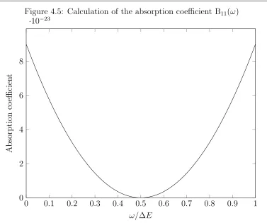
Figure 4.5: Calculation of the absorption coefficient B11(ω)
0 0.1 0.2 0.3 0.4 0.5 0.6 0.7 0.8 0.9 1 0
2 4 6 8
·10−23
ω/∆E
Absorption
co
efficien
t
procedure of integrating over the bounds of the frequency leads us to an absorption coefficient of
B11 = 5.28(4)×10−7m6J−2s−3 (4.66)
Using this value we can calculate the gain rate of a system for several different sce-narios using the expression for the gain rate
N =B11ρ1ρ2 (4.67)
where
ρi =
8πh c3
(ehνi/kT −1)−1ν3
i (4.68)
of the absorbed photons must sum up to the transition frequency, when we fix one we therefore fix the other by
ω2 =ωHF S−ω1 (4.69)
This however does not remove this fact when we integrate over the frequency range where a delta function is present. When this occurs we simply use the fact that
Z ∞
−∞
f(x)δ(y−x)dx=f(y) (4.70)
so we can simply evaluate our expression at the two frequencies we wish such that the total frequency is still equal to the hyperfine transition energy. This would lead to a total expression for the gain rate of
N =
8πh c3
(ehνi/kT−1)−1ν3
1
8πh c3
(ehνi/kT−1)−1ν3
2
4π2e4
~2
M−γγ(i→f)
2
(4.71)
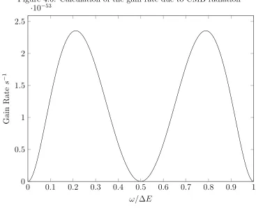
Figure 4.6: Calculation of the gain rate due to CMB radiation
0 0.1 0.2 0.3 0.4 0.5 0.6 0.7 0.8 0.9 1 0
0.5 1 1.5 2 2.5
·10−53
ω/∆E
Gain
Rate
s
−
1
Figure 4.7: Calculation of the gain rate due to CMB radiation and a star
0 0.1 0.2 0.3 0.4 0.5 0.6 0.7 0.8 0.9 1 0
1 2 3 4 5 6 7 8
·10−50
ω/∆E
Gain
Rate
s
−
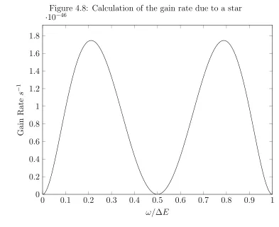
Figure 4.8: Calculation of the gain rate due to a star
0 0.1 0.2 0.3 0.4 0.5 0.6 0.7 0.8 0.9 1 0
0.2 0.4 0.6 0.8 1 1.2 1.4 1.6 1.8
·10−46
ω/∆E
Gain
Rate
s
−
1
4.5
Raman Scattering
however the initial and final state are different and the photon that is emitted is of a different frequency to the one that was absorbed. This can be summed up as an inelastic process. In practice this will change the transitional integrals to account for the fact that the second photon is emitted instead of absorbed.
M−γγ(i→f) = −1
3(e2×e1)
X
n
hnp|z|1si2
ω3/2−1/2
ω2
p0+ 2ωp0ω1+ω12
− ω3/2−1/2 ω2
p0−2ωp0ω2+ω22
(4.72)
This change is to switch the usual plus sign next to the frequency of the photon with a minus sign. In addition to this the frequency of the absorbed photon is no longer bound by the transition energy. The photon can have any frequency so long as it is greater than the transition energy for the hyperfine splitting. The emitted photon however is bound by conservation of energy.
ω2 =ω1−ωHF S (4.73)
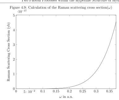
This is due to the fact that the process is inelastic and the energy is lost in the decay to a more excited state than the original. In addition to this a resonance term occurs as the frequency of the incident photon approaches the transition frequency to the first p-state so we will constrain our values for the absorbed photon below this [26]. The equation for the Raman scattering cross section is therefore [11]
σ = (α
2m
ec2)28πa20
3(c)4 ω1ω 3 2
M−γγ(i→f)
2
(4.74)
Figure 4.9: Calculation of the Raman scattering cross section(ω)
0 5·10−2 0.1 0.15 0.2 0.25 0.3 0.35
0 1 2 3 4 5
·10−17
ω in a.u.
Raman
Scattering
Cross
Section
(yb)
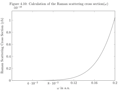
of 0.325 a.u. A closer inspection of the values farther below resonance can be seen in Fig.4.10. As can be seen there is a large exponential scaling with respect to the energy of the absorbed photon.
Even with the increased energy range allowing frequencies that are beyond the hyperfine splitting transition our value for the theoretical Raman scattering cross section is very small. We can see that even across the entire frequency range below resonance we never leave the range of yoctobarns. It would be nearly impossible to see this phenomenon in the laboratory.
4.6
Z-scaling
As with most things calculated for hydrogen, these values can be extended to hydro-genlike ions. Due to the large scaling of the hyperfine transition frequency with Z
Figure 4.10: Calculation of the Raman scattering cross section(ω)
4·10−2 8·10−2 0.12 0.16 0.2
0 0.2 0.4 0.6 0.8 1
·10−18
ω in a.u.
Raman
Scattering
Cross
Section
(yb)
ions to see if our values scale just as well. To do this we look at the Z scaling of the individual values. The transition operator in this case is
z =rcosθ (4.75)
and we know that the particular Z scaling for r is
r ∝ 1
Z (4.76)
and the energies have a Z scaling of
Difficulty arises in extending this simple scale factor to the actual hyperfine splitting in hydrogenlike ions as although this value scales with Z3 it is also dependent on the nuclear magnetic momentµN and the value for the spin of the nucleusI. These values do not have any set scaling so we will be using a combination of literature values as well as a fit to calculate the values for the hyperfine splitting in hydrogenic ions. For the purposes of this work we will be restricting ourselves to stable atoms as we wish to apply this to a laboratory setting. In addition to this due to complications with the coupling of J and I in the intermediate state we will be restricting ourselves further to only ions with nuclear spin I = 1/2. However even with these restrictions we still have 23 separate ions to work with. Due to the location of the hyperfine splitting ω
in the equation, we cannot simply apply an overall multiplying factor to our values and each must be computed individually for each ion. The scale factors that can be applied will be seen in the equation
M−γγ(i→f) = −1
3(e2×e1)
X
n 1
Z2 hnp|z|1si 2
Z4ω3/2−1/2
Z4ω2
p0+Z22ωp0ω1+ω21
− Z
4ω 3/2−1/2
Z2ω2
p0 +Z22ωp0ω2+ω22
(4.78)
When calculating the hyperfine splitting energy for the ground state we use the fact that the Fermi-contact term scales with Z3 as well as with the nuclear magnetic
moment µn so we can take a guess at the correct value through the equation
ωZHF S =ωHHF S∗Z3 ∗
µn
µH
(4.79)
our final approximation of the hyperfine splitting frequency for hydrogenlike ions is
ωZHF S =
ωHHF SZ3µµHn
−0.00566Z + 1.020373 (4.80)
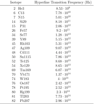
The results of this calculation for all stable isotopes with spin 1/2 can be seen in Table 4.1.
Table 4.1: Hyperfine transition frequency for stable hydrogenlike isotopes with spin 1/2 nuclei.
Isotope Hyperfine Transition Frequency (Hz) 2 He3 8.53·109
6 C13 7.78·1010
7 N15 5.01·1010
14 Si29 8.18·1011 15 P31 2.06·1012
26 Fe57 9.2·1011
34 Se77 1.28·1013 39 Y89 5.15·1012
45 Rh103 5.31·1013
47 Ag109 9.07·1012 48 Cd111 4.44·1013
50 Sn1115 7.86·1013
52 Te125 8.68·1013 54 Xe129 8.65·1013
69 Tm169 6.07·1013
70 Yb171 1.37·1014
74 W183 4·1013
76 Os187 2.42·1013
78 Pt195 2.52·1014 80 Hg199 2.3·1014
81 Tl203 7.73·1014
82 Pb207 2.96·1014
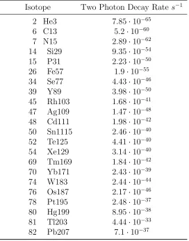
Table 4.2: Ground state hyperfine two-photon decay rate for hydrogenlike stable isotopes with spin 1/2 nuclei.
Isotope Two Photon Decay Rate s−1
2 He3 7.85·10−65
6 C13 5.2·10−60
7 N15 2.89·10−62 14 Si29 9.35·10−54
15 P31 2.23·10−50
26 Fe57 1.9·10−55 34 Se77 4.43·10−46
39 Y89 3.98·10−50
45 Rh103 1.68·10−41 47 Ag109 1.47·10−48
48 Cd111 1.98·10−42
50 Sn1115 2.46·10−40 52 Te125 4.41·10−40
54 Xe129 3.14·10−40
69 Tm169 1.84·10−42 70 Yb171 2.43·10−39
74 W183 2.44·10−44
76 Os187 2.17·10−46 78 Pt195 2.48·10−37
80 Hg199 8.95·10−38
81 Tl203 4.44·10−33 82 Pb207 7.1·10−37
We can as before use the relationship between the Einstein A and B coefficient to arrive at Z-scaled values for the absorption coefficient B in Table 4.3. These values are reported in atomic units as they have dimensions that can be cumber-some and it seems to be the most clear way to report it. They have dimensions of
Distance6Energy−2time−3. As can be seen in Table 4.3 the values don’t seem to change much asZ is increased. This is likely due to the fact that the absorption coef-ficient does not scale as well with the hyperfine transition energy as it does with the overall energy difference between the ground state and the first intermediate state.
Table 4.3: Ground state hyperfine two-photon absorption coefficient for hydrogenlike stable isotopes with spin 1/2 nuclei.
Isotope Two Photon Absorption Rate a.u. 2 He3 2.74·10−30
6 C13 3.17·10−31
7 N15 2.46·10−32 14 Si29 4.2·10−31
15 P31 3.88·10−30
26 Fe57 4.21·10−33 34 Se77 1.34·10−30
39 Y89 2.88·10−32
45 Rh103 1.01·10−29 47 Ag109 3.54·10−32
48 Cd111 3.5·10−30
50 Sn1115 1.41·10−29 52 Te125 1.39·10−29
54 Xe129 1.01·10−29
69 Tm169 4.93·10−31 70 Yb171 5·10−30
74 W183 8.05·10−32
76 Os187 1.44·10−32 78 Pt195 1.32·10−29
80 Hg199 8.15·10−30
81 Tl203 3.11·10−28 82 Pb207 1.43·10−29
Table 4.4: Raman scattering cross of the ground state hyperfine transition in hydro-genlike 2He3.
Energy of the Absorbed Photon(a.u.) Cross Section (yb) 0.128 2.82·10−22 0.256 1.81·10−20
0.384 2.06·10−19
0.512 1.16·10−18 0.64 4.41·10−18
0.768 1.32·10−17
0.896 3.32·10−17 1.024 7.4·10−17
1.152 1.5·10−16
1.28 2.82·10−16
Table 4.5: Raman scattering cross of the ground state hyperfine transition in hydro-genlike 6C13.
Energy of the Absorbed Photon(a.u.) Cross Section (yb) 1.152 2.28·10−20
2.304 1.46·10−18 3.456 1.67·10−17
4.608 9.35·10−17
5.76 3.57·10−16 6.912 1.07·10−15
8.064 2.69·10−15
9.216 6·10−15 10.368 1.22·10−14
Table 4.6: Raman scattering cross of the ground state hyperfine transition in hydro-genlike 7N15.
Energy of the Absorbed Photon(a.u.) Cross Section (yb) 1.568 4.23·10−20 3.136 2.71·10−18
4.704 3.08·10−17
6.272 1.73·10−16 7.84 6.6·10−16
9.408 1.98·10−15
10.976 4.98·10−15 12.544 1.11·10−14
14.112 2.25·10−14
15.68 4.23·10−14
Table 4.7: Raman scattering cross of the ground state hyperfine transition in hydro-genlike 14Si29.
Energy of the Absorbed Photon(a.u.) Cross Section (yb) 6.272 6.75·10−19
12.544 4.33·10−17 18.816 4.93·10−16
25.088 2.77·10−15
31.36 1.06·10−14 37.632 3.16·10−14
43.904 7.95·10−14
50.176 1.78·10−13 56.448 3.6·10−13
Table 4.8: Raman scattering cross of the ground state hyperfine transition in hydro-genlike 15P31.
Energy of the Absorbed Photon(a.u.) Cross Section (yb) 7.2 8.9·10−19 14.4 5.7·10−17
21.6 6.5·10−16
28.8 3.65·10−15
36 1.4·10−14
43.2 4.16·10−14
50.4 1.05·10−13 57.6 2.34·10−13
64.8 4.74·10−13
72 8.9·10−13
Table 4.9: Raman scattering cross of the ground state hyperfine transition in hydro-genlike 26Fe57.
Energy of the Absorbed Photon(a.u.) Cross Section (yb) 21.632 8.05·10−18
43.264 5.15·10−16 64.896 5.85·10−15
86.528 3.3·10−14
108.16 1.26·10−13 129.792 3.76·10−13
151.424 9.45·10−13
173.056 2.11·10−12 194.688 4.28·10−12
Table 4.10: Raman scattering cross of the ground state hyperfine transition in hydro-genlike 34Se77.
Energy of the Absorbed Photon(a.u.) Cross Section (yb) 36.992 2.36·10−17 73.984 1.51·10−15
110.976 1.72·10−14
147.968 9.65·10−14 184.96 3.68·10−13
221.952 1.1·10−12
258.944 2.77·10−12 295.936 6.15·10−12
332.928 1.25·10−11
369.92 2.36·10−11
Table 4.11: Raman scattering cross of the ground state hyperfine transition in hydro-genlike 39Y89.
Energy of the Absorbed Photon(a.u.) Cross Section (yb) 48.672 4.08·10−17
97.344 2.61·10−15 146.016 2.97·10−14
194.688 1.67·10−13
243.36 6.35·10−13 292.032 1.9·10−12
340.704 4.8·10−12
389.376 1.07·10−11 438.048 2.17·10−11
Table 4.12: Raman scattering cross of the ground state hyperfine transition in hydro-genlike 45Rh103.
Energy of the Absorbed Photon(a.u.) Cross Section (yb) 64.8 7.2·10−17 129.6 4.62·10−15
194.4 5.25·10−14
259.2 2.96·10−13
324 1.13·10−12
388.8 3.37·10−12
453.6 8.5·10−12 518.4 1.9·10−11
583.2 3.84·10−11
648 7.2·10−11
Table 4.13: Raman scattering cross of the ground state hyperfine transition in hydro-genlike 47Ag109.
Energy of the Absorbed Photon(a.u.) Cross Section (yb) 70.688 8.6·10−17
141.376 5.5·10−15 212.064 6.25·10−14
282.752 3.52·10−13
353.44 1.35·10−12 424.128 4.01·10−12
494.816 1.01·10−11
565.504 2.26·10−11 636.192 4.57·10−11
Table 4.14: Raman scattering cross of the ground state hyperfine transition in hydro-genlike 48Cd111.
Energy of the Absorbed Photon(a.u.) Cross Section (yb) 73.728 9.35·10−17 147.456 6·10−15
221.184 6.8·10−14
294.912 3.83·10−13 368.64 1.46·10−12
442.368 4.36·10−12
516.096 1.1·10−11 589.824 2.45·10−11
663.552 4.97·10−11
737.28 9.35·10−11
Table 4.15: Raman scattering cross of the ground state hyperfine transition in hydro-genlike 50Sn115.
Energy of the Absorbed Photon(a.u.) Cross Section (yb)
80 1.1·10−16
160 7.05·10−15
240 8·10−14
320 4.51·10−13
400 1.72·10−12
480 5.15·10−12
560 1.3·10−11
640 2.89·10−11
720 5.85·10−11