University of Windsor University of Windsor
Scholarship at UWindsor
Scholarship at UWindsor
Electronic Theses and Dissertations Theses, Dissertations, and Major Papers
1-1-1980
Computation of electric fields in and around high voltage
Computation of electric fields in and around high voltage
insulators.
insulators.
Mohammad Javed Khan
University of Windsor
Follow this and additional works at: https://scholar.uwindsor.ca/etd
Recommended Citation Recommended Citation
Khan, Mohammad Javed, "Computation of electric fields in and around high voltage insulators." (1980). Electronic Theses and Dissertations. 6761.
https://scholar.uwindsor.ca/etd/6761
HIGH VOLTAGE INSULATORS
A Thesis
Submitted to the Faculty of Graduate Studies Through the Department of Electrical Engineering in Partial Fulfilment of the Requirements for the
Degree of Master of Applied Science at the University of Windsor
by
Mohammad Javed Khan
Windsor, Ontario Canada
UM I Num ber: E C 5 4 7 4 4
IN FO R M A TIO N T O USER S
The quality of this reproduction is dependent upon the quality of the copy submitted. Broken or indistinct print, colored or poor quality illustrations and photographs, print bleed-through, substandard margins, and improper alignment can adversely affect reproduction.
In the unlikely event that the author did not send a complete manuscript
and there are missing pages, these will be noted. Also, if unauthorized copyright material had to be removed, a note will indicate the deletion.
UMI Microform E C 5 4 7 4 4 Copyright 2 01 0 by ProQuest LLC
All rights reserved. This microform edition is protected against unauthorized copying under Title 17, United States Code.
ProQuest LLC
789 East Eisenhower Parkway P.O. Box 1346
The application of the charge simulation technique to
multiple dielectric systems (two-dielectric) is the focus of
this effort. The electric field distribution is evaluated in
and around insulator elements used on practical high voltage
transmission lines. For this purpose, two insulators namely
a Suspension Insulator section and a Long Rod Polymer
Insulator were studied. The agreement of some experimental
results obtained elsewhere with the computed ones for the long
rod insulator is of the order of the accuracy with which
measurements of potential can be made. A detailed study of
the errors and discrepancies arising in the field conditions
in the resulting models is presented. Suggestions for the
application of the method in high voltage insulator design
ACKNOWLEDGEMENTS
I am most grateful to Professor Philip Alexander and
express my sincere appreciation to him for suggesting the
problem, for his supervision of this work and of course for
his tireless reading of this dissertation in manuscript.
I am also indebted to Mr. M. D. Baillargeon, academic \
programmer, Computer Centre, University of Windsor for his
help in detecting errors in the computer programs.
Thanks are also extended to Mr. W. A. Chisholm, Engineer
Transmission and Special Projects Section, Electrical Research
Department, Ontario Hydro, for allowing the presentation of
their experimental results for the long rod polymer
insulator.
Finally, I would like to thank my parents and my complete
family tree, not for having anything to do with the compilation
of this thesis, but for helping to further my career either
Page
ABSTRACT ii
ACKNOWLEDGEMENTS iii
TABLE OF CONTENTS iv
LIST OF FIGURES viii
LIST OF TABLES xii
I . INTRODUCTION 1
1.1 Preamble 1
1.2 Statement of Problem 3
1.3 Organization of Thesis 5
II. REVIEW OF LITERATURE 9
2.1 General 9
2.1*1 Electrode Surface Subsectioning 11
2.1.2 Interior Placement of Charges 12
2.2 Charge Simulation Technique 12
2.2.1 Conventional Method 12
2.2.2 Application to Single Dielectric 15
Systems
2.2.2.1 High Voltage Electrodes 15
2.2.2.2 Transmission Lines 16
2.2.3 Application to Multiple Dielectric 19
Systems
2.3 Accuracy of the Method 2 2
2.4 Computation Time Requirements 24
Table of Contents Cont'd
Page
III. PRELIMINARY ANALYSIS 29
3.1 General 2 9
3.2 Basic Principles 31
3.2.1 Principle of Calculation 33
3.2.2 Application Example 37
3.2.3 Programming 40
3.3 Results 42
3.3.1 Conclusions 47
IV. PROBLEM FORMULATION 58
4.1 General 58
4.2 Calculation for Two-Dielectric Arrangements 60
4.2.1 Computation Procedures 62
4.2.2 Equation Formulation 64
4.2.3 Choice of the Method for solving 09
Linear System of Equations
4.3 Mathematical Formulation 73
4.3.1 Cubic Spline Interpolatory Scheme 73
4.4 Application of the Method to Practical 75
High Voltage Insulators
4.4.1 Suspension Insulator 75
4.4.2 Long Rod Polymer Insulator 78
V. RESULTS AND DISCUSSIONS 84
5.1 General 84
5.2 Suspension Insulator 88
5.2.1 Metallic Parts of the Insulator Exposed 88
to Air
5.2.2 Metallic Parts Interfaced with the 88
5.2.3 Potential Discrepancy along the Dielectric Skirt
5.2.4 Discrepancy in the Tangential Field along the Dielectric Skirts
5.2.5 Potential Distribution along the Dielectric Skirts
5.2.6 Programming
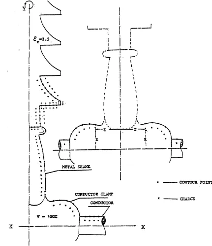
5.3 Long Rod Polymer Insulator
5.3.1 General
5.3.2 Metallic Parts of the Insulator Exposed to Air
5.3.3 Metallic Parts Interfaced with the Dielectric
5.3.4 Potential Discrepancy along the Dielectric Skirts
5.3.5 Discrepancy in the Tangential Field along the Dielectric Skirts
5.3.6 Potential Distribution along the Polymer Rod
5.3.7 Experimental Results
5.3.8 Programming
VI. CONCLUSIONS AND RECOMMENDATIONS
6.1 General
6.2 Conclusions
6.3 Recommendations
APPENDIX A Expressions for Potential and Field
Strength due to Point, Line, Ring Charge
APPENDIX B Computer Program for Suspension
Table of Contents Cont'd
Page
APPENDIX C Computer Program for Long Rod Polymer 173
Insulator
BIBLIOGRAPHY 185
Figure Page
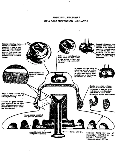
1.1 Practical Suspension Insulator 5
1.2 Long Rod Polymer Insulator 7
2.1 Suspension Insulator simplified to a Truncated 21
Cone
3.1 Pin of a Practical Suspension Insulator 30
3.2 Hemispherically Capped Cylinder 32
3.3 Principle of the Charge Simulation Method 34
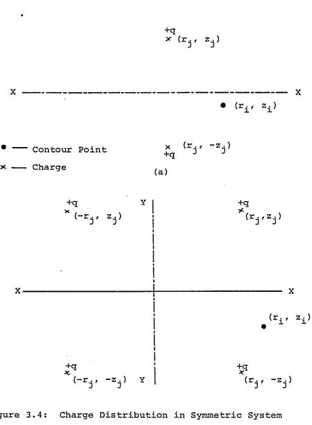
3.4 Charge Distribution in Symmetric System 38
3.5 Flow Chart 41
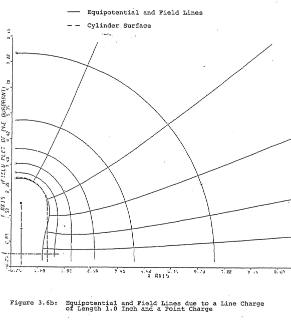
3.6 Equipotential and Field Lines due to a Line 46-50
(a-e) and a Point Charge
3.7 Equipotential and Field Lines due to a Point 54-56
(a-c) Charge and Discrete Line Charges
4.1 Procedure for Computation of Fields and 63
Potentials of a Two Dielectric System
4.2 Matrix Representation of Equations Described 68
in Section 4.2.2 for Suspension Insulator
4.3 Distribution of Charges in the Suspension 77
Insulator
4.4 Distribution of Charges in the Partial 81
Configuration of Long Rod Polymer Insulator
4.5 Charge Distribution in the Conductor Clamp 83
of the Polymer Insulator and their Positive Images
5.1 Potential Error along the Air Side of the Cap 8 7
5.2 Potential Error along the Air Part of the Pin 8 9
5.3 Potential Error along the Conductor-Air 90
Interface of the Pin
5.4 Potential Error along the Vertical Surface of 91
List of Figures Cont'd
Figure Page
5.5 Potential Error along the Top Horizontal 93
Conductor-Dielectric Interface of the Pin
5.6 Potential Error along the Horizontal 94
Conductor-Dielectric Interface of the Cap
5.7 Potential Error along the Vertical Interface 95
of the Cap with Dielectric
5.8 Potential Discrepancy along the Upper skirt 97
5.9 Discrepancy in Potential along the Lower Skirt 98
5.10 Ring Charge Representation in the Lower 1.Q0
Dielectric Skirt
5.11 Discrepancy in Tangential Field along the 101
Upper Skirt
5.12 Discrepancy in Tangential Field along the 10 3
Lower Skirt
5.13 Potential Distribution along the Upper Skirt 105
5.14 Potential Distribution along the Lower Skirt 106
5.15 Flow Chart 107
5.16 Distribution of Charges in the Long Rod 109
Insulator
5.17 Potential Error along the Air Part of the High 113
Voltage Metal Shank
5.18 Potential Error along the Conductor Clamp and 115
a Section of the High Voltage Conductor (5.0 cm)
5.1-9 Potential Error along the Metal Shank of the 116
Grounded Conductor
5.20 Potential Error along the Conductor-Dielectric 117
Interface of the High Voltage Conductor
5.21 Potential Error along the Conductor-Dielectric 119
Interface of the Grounded Conductor
5.22 Potential Discrepancy along the Vertical Column 12 0
of the Polymer Rod
5.23 Potential Discrepancy along the Horizontal 121
Figure 5. 24 5. 25 5.26 5.27 5.28 5.29 5.30 5. 31 5.32 5.33 5. 34 5. 35 5.36 5. 37 5. 38 5. 39 5.40
Potential Discrepancy along the Vertical and Sloped Skirt (Unit #1)
Potential Discrepancy along the Horizontal Interface (Unit #2)
Potential Discrepancy along the Vertical and Sloped Skirt (Unit #2)
Potential Discrepancy along the Horizontal Interface (Unit #3)
Potential Discrepancy along the Vertical and Sloped Skirt (Unit #3)
Discrepancy in Tangential Field along the Vertical Column of the Polymer Rod
Discrepancy in Tangential Field along the Horizontal Interface (Unit #1)
Discrepancy in Tangential Field along the Vertical and Sloped Skirt (Unit #1)
Discrepancy in Tangential Field along the Horizontal Interface (Unit #2)
Discrepancy in Tangential Field along the Vertical and Sloped Skirt (Unit #2)
Discrepancy in Tangential Field along the Horizontal Interface (Unit #3)
Discrepancy in Tangential Field along the Vertical and Sloped Skirt (Unit #3)
Potential Distribution along the Vertical Column of the Polymer Rod
Potential Distribution along the Horizontal Interface of the Polymer Rod (Unit #1)
Potential Distribution along the Vertical and Sloped Skirt (Unit #1)
Potential Distribution along the Horizontal Interface (Unit #2)
Potential Distribution along the Vertical and Sloped Skirt (Unit #2)
List of
Figure
5.41
5.42
5.43
5.44
Figures
page
Potential Distribution along the Horizontal 142
Interface (Unit #3)
Potential Distribution along the Vertical 143
and Sloped Skirt (Unit #3)
Computed Potential Distribution of a Long 144^
Rod Insulator
Comparative Results of Potentials on First 14 6'
Table
3.1 Effect of Length of Line Charge on Error
3.2 Effect of the Position of Boundary Point on
the Hemisphere on Error with varying Length of Line Charges
3.3 Effect of the Number of Charges on Error
5.1 M.S. and R.M.S. Error on Parts of the Partial
Configuration of the Rod Insulator (Fig. 6.6a)
Page
45
52
53
I . INTRODUCTION
1.1 Preamble
The term "high voltage insulator" designates, in general,
all devices that serve for the insulation of conductors at
high potential from ground. They can be grouped as bushings,
interior supports and line insulators. In the early days of
electrical distribution of power the insulator problem was
unimportant. The insulator gave more satisfactory service
than the rest of the apparatus essential to the generation
and distribution systems. As long as the voltages were low
the electric field distribution was of relatively small
importance. As the transmission distances and therefore,
the economic transmission line voltages, increased the
insulator problem became more acute. As a result, with the
increased voltages came an increasing amount of insulator
trouble resulting in frequent failures of electric power
systems at a rate that for a time threatened the success of
high voltage transmission of electrical energy [1].
During the past few years there has been a remarkable
development throughout the world in high voltage transmission
systems. With the growing demand for electrical energy, the
present trend is to transmit large blocks of power at an ultra
high voltage (UHV*) level which further necessitates the
thorough investigation of the insulation problem of transmission
lines for successful operation with minimum interruptions.
voltage are the appearance of extremely high electric fields
near the conductor surface as well as on some grounded
surfaces. Due to extremely high electric field, radio
interference and audible noise generated may reach levels
higher than those permitted by regulations or higher than
desirable. An important problem associated with EHV/UHV lines
is the occurrence of corona around the conductor surface [2].
Corona is considered as the partial breakdown of air
surrounding the metallic parts of the insulator and line
conductors. The electric power used in ionizing the air
surrounding the conductor parts of the insulator is known as
corona loss [3]. The corona loss represents a loss of revenue
and therefore it must be minimized for economical reasons.
When high voltage transmission lines are in normal
operation, small spark discharges occur on the insulators
even in clean dry conditions [4]. These discharges, in common
with all spark discharges, contain components of radio frequency,
so that a radio-frequency disturbing field is radiated from the
line conductors. If the discharges became more intense
because of humid weather, contaminated insulators, or faulty
contact between the hardware and the porcelain, the intensity
of the radiation increases, and may interfere with the
reception of radio signals by receivers in the vicinity of
the line.
In recent years, the problem of radio interference has
3
systems and partly owing to the high sensitivity of modern
receivers. A well insulated high voltage line, properly
maintained, is not a serious source of interference, but
intense interference can arise if an abnormal discharge is
present. The insulator should therefore be free from
discharges at a voltage which is usually specified at 20 to
40 percent above the phase to earth voltage [5].
Recognizing the importance of providing adequate
insulation strength to high voltage transmission systems,; it
is essential to have an accurate knowledge of the electric
field distribution in and around high voltage insulators.
This knowledge of the electric field distribution can
also be applied to the determination of breakdown strength
of the insulator material as well as corona noise generation
susceptibility and is of great help to the designer of EHV and
UHV transmission lines.
1.2 Statement of Problem
In general there are two types of transmission line
insulators - Pin type and Suspension type.
The use of Pin type insulators is limited to voltages
below 50 kV since at high voltages they become uneconomical;
the cost increases rapidly as the voltage increases and
is proportional to V* where x is greater than 2 [6]. A
further disadvantage of Pin type insulators is that
replacements are expensive. For these reasons high voltage
lines are insulated by suspension insulators in which case,
Several important advantages result from this system:
1) Each insulator is designed for a comparatively low
working voltage and the required total insulation is
obtained by using a "string” of a suitable number of such
insulators.
2) In the event of failure of an insulator, one unit
instead of the whole string, may need to be replaced.
3) The mechanical stresses are reduced since the line
is suspended flexibly; with Pin type insulators the rigid
nature of the attachment results in fatigue and ultimate
brittleness of „ the conductor due to the intermittent nature
of the stress due to wind loads. Also, since the string is
free to swing, there is an equalization of the tensions in
the conductors of successive spans.
4) In the event of an increase in the operating voltage
of a line, the insulation requirements can be met by adding
the appropriate number of units to the string instead of
replacing all insulators as would be made necessary with the
Pin type.
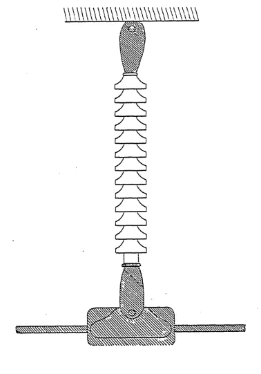
Owing to the present day wide application of Suspension
insulators for high voltage transmission systems, a Suspension
insulator of Canadian Ohio Brass Company Limited (Catalogue
-71, page 11, 1977) as shown in Fig. (1.1) is considered for
the analysis of electric field distribution.
shown in Fig. (1.2} called a long rod polymer insulator is
also analyzed. This unit is under development by Ontario
Hydro and has not yet been installed on actual high
voltage transmssion lines, being in the experimental process.
Transmission line insulators must bear the flashover
stress under very difficult circumstances, namely dry, wet
and polluted conditions. Line insulator’s shapes have
become complicated chiefly because of this requirement. The
thickness of the insulation between the metallic parts of the
insulator and the length of the sparking distance are not the
only factors which decide the electrical performance of an
insulator, but the distribution of the electrostatic field
and equipotential surfaces is also of considerable importance
in determining corona formation and flashover voltage.
The purpose of this thesis is therefore to compute the
electric field distribution in and around high voltage suspen
sion insulators used on practical high voltage transmission
lines. This knowledge of the electric field distribution also
enables us to determine the breakdown strength of the
insulator material.
1* 3 Organization of Thesis
Chapter II gives a detailed and thorough review of the
available literature on the Charge Simulation Technique used
for the calculation of electric fields in high voltage systems.
The application of the technique to single dielectric systems
-high voltage electrodes, transmission lines and multiple
Lacking cattar key. Humi annpa under theuldor In cap In hnld (irmly In teated decked] p m itln n . Spread m d i prevent lu ll withdrawal and five braadnr bearing turface undnr ball whan lacked.
Lackad baikceckat caw- nectien. W itt cattaf kay secured In its advanced paaitlan. vertical m an * m anl af lha b a ll la re* ttrlc ta d and tha Jaitat canned ba dlsataamblad u n til tha sattar kay la withdrawn.
Cattar key In lackad paaitlan. Hump balaw tha aya, ahawn In view at la lt prevent* tha kay Iram Paw* accidantalty ratractad
In laekad paaitlan. haad a I cattar kay la fluah ta lurfaaa ef cap. Tha haia ia racaaaad ta parmit aaay accaaa with a haakad hand ar hot line tsel la withdraw tha cattar. Sandad turlacaa an
partalain aaaambly
l<
Elaatla aapanalan and can* traction at cap matal raact ta •ppllcatian af lead and draw parti back ta normal relation* ahlp at end af a lead cycle. (Movement yreatiy exaggerated) Matal in bath cap and pin
prelected by heavy caat af hat-dlp galvaaiiing.
Cap and pin leametry can* varta axial lead an the Ineu* later Inta pure cempreaalen land an tha wall ef tha p area- lain haad sectien.
Danaa. strong. rlectm al preaaea porcelain.
farted Aaaamblad with ttaana-curad,
neat partland cement Catalogue Rating and year of
manufacture imprinted on top surface of Porcelain Oise. Tradamark appeare on Cap.
shown in Fig. Cl*2) called a long rod polymer insulator is
also analyzed. This unit is under development by Ontario
Hydro and has not yet been installed on actual high
voltage transmssion lines, being in the experimental process.
Transmission line insulators must bear the flashover
stress under very difficult circumstances, namely dry, wet
and polluted conditions. Line insulator's shapes have
become complicated chiefly because of this requirement. The
thickness of the insulation between the metallic parts of the
insulator and the length of the sparking distance are not the
only factors which decide the electrical performance of an
insulator, but the distribution of the electrostatic field
and equipotential surfaces is also of considerable importance
in determining corona formation and flashover voltage.
The purpose of this thesis is therefore to compute the
electric field distribution in and around high voltage suspen
sion insulators used on practical high voltage transmission
lines. This knowledge of the electric field distribution also
enables us to determine the breakdown strength of the
insulator material.
1.3 Organization of Thesis
Chapter XX gives a detailed and thorough review of the
available literature on the Charge Simulation Technique used
for the calculation of electric fields in high voltage systems.
The application of the technique to single dielectric systems —
high voltage electrodes, transmission lines and multiple
8
The accuracy of the method and the computation time requirements
are also reviewed and conclusions have been derived.
Chapter III presents a preliminary analysis. A simple
example of a hemispherically capped cylinder is demonstrated
using a combination of point and line charges. The
effect on the potential distribution of the number of charges,
position of the boundary point (on the hemisphere of the
cylinder), and the length of the line charge segment is studied
and conclusions have been derived.
Chapter IV is on the mathematical formulation of the
problem. The equations necessary for simulation (two dielectric
system only) are presented. The charge distribution in the
suspension and long rod insulator are illustrated in separate
sections. The rotationally non-symmetric problem of a rod
insulator is approached making use of the partial symmetry present.
Chapter V is devoted to 'Results and Discussions'.
Results for the suspension and long rod insulator are presented
and discussed in separate sections. The experimental results
obtained by Ontario Hydro for the long rod insulator are
compared with the computed on e s .
Chapter VI provides 'Conclusions and Recommendations'.
In this chapter, important conclusions are presented and
2.1 General
The knowledge of the electric field distribution in
the design of any high voltage system component is important.
An error of a few percent in the estimation of the field and
potential distribution may result in an unacceptable loss of
accuracy / efficiency in the manufactured device or even the
failure of the device. The prior knowledge of the field
distribution will therefore accurately predict the design
parameters and performance evaluation of devices by means of
purely computational techniques.
There are several techniques that have been used to
numerically calculate electrostatic field distributions. The
calculation of electric fields requires the solution of
Laplace's and Poission's equations with boundary conditions
satisfied. This can be done either by analytical or numerical
methods. However, in many cases physical systems are so
complicated that analytical solutions are seldom applicable
and hence numerical methods are commonly used for such
applications [7, 8].
There are two distinct numerical techniques reported in
the literature. The first method is based on difference
techniques employing Laplace's and Poission's equations in
the space where the field is desired to be evaluated. This
10
Laplace's equation is then approximated within each small
region by equations which relate the unknown potential of
the region to the unknown potential in other regions and to
known boundary potentials.
Many papers have been published on the solution of
Laplace's equations by the Finite Difference Method and the
Finite Element Method and they have been very extensively
described in the literature [9, 10].
Difference' techniques are very powerful when the region
of interest contains a number of different materials or a
dielectric constant which varies in space [11]. In more
simple cases (such as the case where only conductors are
present), Difference techniques may be more cumbersome than
necessary due to the large number of linear equations that
must be solved [12]. Furthermore, finite element and
difference techniques are useful only in bounded regions,
whereas, many physical problems of interest are unbounded.
However, attempts have been made to use Difference techniques
for the solution of electric field problems where the field
is not bounded in space but extends infinitely far [13, 14].
In this method, an artificial finite boundary condition is
initially introduced to allow solution and then iteratively
removed, as the solution proceeds. In order to have a
minimum effect of errors in the known potentials on the
calculated potential values in the region of interest, the
artificial boundary must be located far enough away from the
Laplace's equations must be solved for a larger region than
the region of interest. Thus a larger number of equations
must be solved which adds to the computational time [15].
The second approach to the computation of fields is
based on integral equations [16, 17].
By an application of Green's identity, Laplacian's
equation ( V 2 V = o ) can be expressed in integral form [18].
This can be done in two ways.
2.1.1 Electrode Surface Subsectioning
The electrode surface is divided into subsections
with their associated charges. It will be assumed here that
the medium consists of several different homogeneous materials
and that as a result, the only charges are the surface charges.
If this is not the case, then volume charges must be considered
[19]. The integral equation can be solved for the surface
charge densities by approximating the integral as a sum on
subsections considered on the entire electrode surface. The
sum is set equal to the known potential at the centre of each
subsection. As a result of this discretization process, a
set of linear algebraic equations is obtained in terms of
unknown segments of charges which when solved with the digital
computer gives values of these charges. This technique is
a special case of the Moment method [20]. Once the charge
densities are obtained, potential and electric field values
2.1.2 Interior Placement of Charges
Discrete charges are placed inside the electrode
surface. The potential of the unknown surface charges is
approximated fay line, ring and point charges (instead of assuming
them to be surface charges) placed at some distance behind
the surface on which the potential is to be matched. The
potentials due to these charges will be well behaved at, and
in front of, the surface and thus can simulate the field of a
surface charge (at least approximately).
This method of discretization is known as the
Charge Simulation technique and was first presented by H.
Singer [21]. In addition to two dimensional field calculations,
Singer has reported results for three dimensional geometries
with and without axial symmetry. He also studied problems
with dielectric-dielectric boundaries.
The work presented in this thesis is based on
Singer's technique of Charge Simulation. A survey of the
available literature on the Charge Simulation technique was
therefore carried out in order to observe the applicability
of the method to coping with field problems associated with
High Voltage devices.
The review is presented in the following sections.
2.2 Charge Simulation Technique
2.2.1 Conventional Method
The Conventional Charge Simulation technique is
of the unknown surface charges is approximated by three forms
of charge arrangments i.e. line, ring and point charges
depending upon the geometry of the High Voltage device at
hand. The only difficulty with this idea of approximating the
surface charges is that potentials near a uniformly charged
surface are bounded, but potentials near line, ring and
point charge are unbounded. In order to overcome this
difficulty, Singer placed equivalent charges at some
distance behind the surface on which the potential is
matched.
The three forms of charge arrangments for a
particular High Voltage electrode configuration have been
seen to cover almost all possible needs of simulation to
cope with the System Configurations [21, 22]. The point
charge, due to its spherically symmetrical field behaviour,
suits spherically symmetrical surfaces; the line charge (finite
or infinite length) suits cylindrical configurations and the
ring charge is used to model axially symmetrical profiles
of High Voltage apparatus. An adequate combination of the
three forms of charge can be made to simulate almost any
practical electrode system [23].
In this method, the actual charge distribution on
the conductor surface is represented by several fictitious line
charges inside the conductor surface and their images represent
the effect of the ground (if considered). These charges can
be placed at any desired position inside the conductor
14
surface, one of the equipotential surfaces resulting from the
fictitious charges and their images must coincide with the
conductor surface. The potential at any point can be
calculated by the superposition of the potential due to the
individual initially unknown fictitious charges. Specifying the
potential at various points on the conductor surface to be
the values of potential desired there, yields a number of
simultaneous equations in terms of the unknown line/ring/point
charges depending upon the geometry at hand. These equations,
when solved give the values of the desired charges. Having
calculated the values of these charges, the potential at many
other points on the conductor surfaces are computed to check
whether the conductor surface results in an equipotential
surface. Thus considering a set of Hm" points selected on a
surface at potential "<f>" and "m" charges considered inside the
conductor(s) leads to a system of "m" linear equations for the
"m" charges as shown below:
n
...
2.1j = 1
(i = 1, f m)
wher e,
n = number of charges in the system
m = number of contour points at which the potential
P . . = the associated potential coefficient
in matrix form,
IP] * [Q] = I<f>c ] ... 2.2
Ordinarily, the number of boundary points "m" is
equal to the number of charges "n11. Given a particular
configuration, the co-efficients P^j will be determined by the
boundary conditions. Once the system of linear equations is
solved for the charges [Q], then it must be determined whether
the calculated set of charges fits the boundary conditions.
For instance, the potential at a number of check points on
the boundary can be calculated. The difference between these
potentials is a measure of the accuracy of the simulation.
The basic principle described above is well known
in Field Theory. Together with suitable ways of discretization,
this known principle forms the basis of electric field computa
tion of two and three dimensional systems as presented by H.
Singer et al [21].
2.2.2 Application to Single Dielectric Systems
2.2.2.1 High Voltage Electrodes
With the increasing variety in the profiles of
high voltage apparatus, more attention is being paid to surfaces
in proximity to these bodies. Sharply tipped termination with
high voltage electrodes are of special importance as they are
16
The charge simulation technique is applied for
the calculation of two-dimensional and three-dimensional
fields with and without axial symmetry. Considerable attention
has been given to electrode configurations used in high voltage
experimentation by many authors. H. Singer [21] calculated
the electric field between a conductor strip and a plane and
the influence of an earthed cage on the field of a sphere-gap
was analyzed as an example of an axial symmetrical problem.
He also explained the principle of the method applied to
three-dimensional fields without axial symmetry by a single
example, a rod-rod gap with a trigger electrode.
Abu - Seada [22] applied the charge simulation
method to the calculation of electric fields of a rod-rod gap.
H. Parekh et al I23J computed electric fields for rotationally
symmetric electrodes and A. Yializis et al [24] calculated
the potential distribution for a rod-plane electrode configura
tion and presented an optimized version of the charge simulation
technique. Masanori et al [25] examined the field distribution
i
of multiple axisymmetric electrodes displacing and rotating
the plane of symmetric model charges. They made calculations
of a three-dimensional axisymmetric gap for a tilted upper
rod - plane electrode arrangement and the rod - plane with lower
rod arrangement. *
2.2.2.2 Transmission Lines
The application of the charge simulation
technique to single dielectric systems finds its greater use
overhead transmission lines. Since the phenomena of corona and
radio interference are more acute with transmission at EHV and
UHV levels, electric field calculations are made for bundle
conductors used for such transmission lines. The first
attempt was made in the early thirties by Crary and reported
by Clarke [26]. C r a r y ’s formulation of electric field was
limited to a ratio of spacing to diameter of subconductors
equal to or greater than five. His formulation was modified
by Poristspy, reported by Clarke, using complex variables
and the transformation techniques but still was not applicable
for a bundle of more than two subconductors. Adams [27]
calculated the electric field for a three phase AC transmission
line. He represented the charge on each conductor by a single
line charge at the centre of the conductor. The effect of
ground was taken into account by considering an image of each
line charge below the ground plane. He calculated first the
values of the line charges by solving simultaneous equations
which related the line charge with the potentials on the
conductor. Once these values of line charges were obtained,
the electric field at any desired point was calculated by
superimposing the contributions due to the individual line
charges. The results obtained by Adams were not accurate
because of the fact that the equipotential surfaces resulting
from the line charges (assumed to be at the centre of the
subconductor) did not coincide with the subconductors
surfaces. This meant that one of the boundary conditions
surfaces was not satisfied.
Sarma and Janischewskyj [28] used the method
of successive images to calculate the electrostatic field of
a system of parallel cylindrical conductors. Their method was
based on the concept of representing the distributed charge
on the conductor's surface by a system of line charges
inside the conductor's surface in such a way that one of the
equipotential surfaces resulting from the line charges
coincided with the conductor surface. Using the process of
successive images, Sarma and Janischewskyj calculated the
electric field around the bundle conductors. The ground
effect was taken into account by placing images of line
charges below the ground plane. Although the values of
electric field obtained by this method were accurate for
higher ratios of r/2s (r = radius of cylinder, 2s = distance
between line charge and the centre of the cylinder), the
number of line charges required to simulate the parallel
conductor system became very large for the electric field
computation for bundle conductor transmission lines.
Abu-Seada and Nasser [29, 30] used the method
of charge simulation to calculate the electric field and
potential around a twin-subconductor bundle. In this
method, the actual charge distribution on each subconductor
surface was represented by several fictitious charges placed
inside each subconductor. These line charges of unknown
magnitude were placed on a fictitious cylinder whose radius
positions of these line charges on the fictitious cylinder
were determined by a trial and error method to achieve better
accuracy of the results. The results obtained by Abu-Seada
and Nasser gave an error of about one percent in the values
of the direction of electric field. However/ their method
was applicable for the case of twin subconductor bundles.
Parekh [31] described a method based on charge simulation which
used arbitrary specifications of location of the images and
boundary points and was applied to bundles of up to eight
cylindrical subconductors.
2.2.3 Application to Multiple Dielectric Systems
In the design of any electrical system, a potential
i
distribution of the system is essential for the calculation
of electric stresses involved. The design may vary from a
simple situation to a more complex one. The advent of
ever faster digital computers has made it possible to synthesize
in great detail hundreds of alternative designs to give
specifications for many types of electrical machines.
Electric machines and high voltage devices often contain
multi-dielectric insulation layers between conductors or cores
etc. For the design of electric insulation of any such
device and for the withstand voltage tests of dielectrics, it
is important to have accurate information of. the electric
field distribution in such systems.
Different approaches have been presented by various
20
systems involving multiple dielectrics, the discussion of
which is beyond the scope of this review.
H. Singer et a l . [21] developed a method of
calculating electric fields in two-dielectric arrangements
which formed the basis of this work. This method will be
explained fully in Chapter IV. As an application of this
method, they applied it to a sphere electrode with a dielectric
slab. For studies of the electric strength of solid
insulating material, flat-slab specimens are often tested by
such arrangements (i.e. a dielectric slab between a sphere and
a plane) [3 4]. As an example, they applied the method to a
practical electrode arrangement used for shielding of high
voltage apparatus. They also applied this method to the
calculation of the field strength at the shielding electrodes
of UHV testing transformers.
Mukerjee and Roy [35] applied the same method of
computation as proposed by Singer to the calculation of
fields in a multiple dielectric, three dimensional system.
They applied the method to a parallel plate arrangement as a
test example and then applied it to a disc insulator. The
insulator shape was simplified to a truncated cone as shown
in Fig. (2.1).
The method of computation in two dielectric media
proposed by Singer received further encouragement from the
researchers. More recently T. Sakakibara [36] applied this
method to the calculation of three dimensional asymmetric
22
simplified post type spacer used in SF_ gas insulated apparatus
was selected as a calculation model. A high voltage impulse
test was also carried out by the authors to varify the validity
of the method and the results were found to be in good agree
ment. Takeshi and Oyozo [37] described a method to determine
the electric field of a point charge by the method of images
in three or more dielectric layers on a plane conductor.
They applied this method in combination with charge simulation
to calculate the field of a spherical conductor situated in
three dielectric layers on a plane conductor. In this
method ring charges in the sphere together with their images
were used for representing the field.
Tadasu [38] described a method to study the field
behaviour near singular points in composite dielectric
arrangements. This paper analyzes the field behaviour of
a contact point of the boundary with an electrode numerically
by the charge simulation method. A comparison with the
analytical solution gave fairly good agreement between
analytical and numerical values.
2.3 Accuracy of the Method
A measure for the accuracy of the model is the "Potential
Error" at various check points on the surface of the electrode
between two adjacent contour points [21]. This "Potential
Error" is defined as the difference between the specified
potential of the electrode and the computed potential.
Experience shows that the error of the electric field is up
[21]. Therefore, the potential error should be less than 0.1%
in an area of the electrode if a field strength accuracy of
1% is desired in this area.
The significance of keeping the "Potential Error" below
0.1 % is important since all corona calculations are very
sensitive to the values of electric fields, a very small
error in the values of electric field might result in a very
large error in the values of the corona onset voltage,
corona loss and radio interference (as estimated by Parekh [39]
even a very small maximum error in the potential (for example
0.2%) does not ensure a small error which can, in the same
region be as large as 3.5 percent). The practical goal for
accuracy in the simulation of electrodes is limited by the
manufacturing tolerences of conductors. Similarly the accuracy
of the simulation of dielectrics has as its practical goal,
the accuracy of the measurement of dielectric constant
values.
One difficulty in using the charge simulation technique
is that the location of equivalent charges is difficult to
obtain analytically [24]. As a result, the location of the
equivalent charges is guided by experience. Thus the
accuracy is usually checked after the problem is solved by
determining how closely the boundary conditions are
matched along all the interfaces. Also the accuracy in the
solution is sensitive to the number of charges chosen for a
particular problem. The larger the number of charges, the
2 4
requirements are of relative importance. Hoy and Mukerjee
[35] reported that for an Air-Dielectric arrangement for a
Disc insulator, an increase in the number of charges modifies
the results but a point is reached beyond which this
increase has no appreciable bearing on the solution on the
conductor or dielectric interfaces. This indicates that the
limit of accuracy has been attained. More recently Beasley et
al.[40] made a comparative study of the three methods, namely
the Charge Simulation Method, the Finite Element Method and
the Monte Carlo method and applied them to different geometries
of a practical engineering nature. They concluded that for
some very large and complex configurations it may not be
possible to obtain satisfactory solutions using only one
method. They suggested that in such cases the Monte Carlo
Method or the Charge Simulation Method may be used to derive
a first approximation followed by the Finite Element Method
within some reduced subregion of interest.
2.4 Computation Time Requirements
The significance of precision in computing potential at
the electrode surface and thereby calculating the error can
not be denied but improving the precision of results beyond a
given limit may not be worth as much as obtaining a given
precision with a maximum saving of computer time and memory
requirements. In this connection, any algorithm aimed at
reducing overall computer time and memory requirements ,
precision being equal, will appear to be extremely valuable
could be reduced, or at a given cost, a more complex problem
could be solved.
Keeping in view this aspect of the problem attempts have
been made by different authors proposing optimization
techniques to reduce notably the cost of numerical field
computation on the basis of a fixed degree of precision required.
A fitting-oriented modification to the charge simulation
method in estimating electric fields is introduced by H.
Anis et. al. [41] which appreciably reduces computation time
and cost. In this method, the multiple linear regression
makes it possible to reduce the size of the simulating charge
system without altering the selected potential boundary
points. Another optimization approach for the computation
of electric fields, based on Charge Simulation technique is
described by A. Yializis et* al. [24]. The objective function
for optimization in this method was the accumulated square
error. The position of charges and their values were chosen
to be the variables of optimization subject to constraints
imposed according to the nature of the problem described. The
objective function was minimized to 1%. However, the
optimization algorithm (Rosenbrok's Optimization Technique)
used by the authors is not the most rapidly converging
technique and therefore savings in computation time did not
result. Fast convergence techniques such as Davidson's method
modified by Fletcher and Powel have been suggested for
reducing computation time with comparable accuracy. Other
26
to the authors [24] are the initial values of the optimization
parameters and the effectiveness of the objective function.
The latter factor is important, since for more complex
configurations it is possible that the minimum accumulated
square error may not be an efficient criterion.
A similar approach but with unconstrained optimization
is presented by Y. L. Chow et a l . [42] and has been applied to
a number of normally encountered geometries in engineering
applications. The objective function assumed in this is the
mean square error of the potentials and the optimization
technique used is due to Fletcher [43] which is one of the
most powerful techniques for unconstrained optimization. The
advantage of using Fletcher's algorithm is that as the
gradient "g" (g = VU, U being the objective function) is
computed, the electric field intensity (E =V(J>) on the
conducting boundary is implicitly obtained. Therefore it can
be extracted without further computation.
A. Mohsen and M. Salam [44] presented a development of
the charge simulation technique for the calculation of electric
field around conductor bundles of EHV transmission lines. In
this method a known initial set of charges is introduced which
are deduced from the analysis of a similar but simpler
problem. These initial charges may be used in addition to a
set of unknown charges which are determined from the boundary
conditions. The better the initial charges, the lower will
be the number of unknown charges. This will lead to a consider
et al.[36] described a modification of the charge simulation
method applicable to three-dimensional asymmetric fields with
two dielectric media Cinitially proposed by Singer [21]).
Since the formulation of a large potential coefficient matrix
results in extensive computation time and memory requirements,
this paper takes advantage of symmetry in the problem
where-ever it exists.
A comparison with the finite difference method shows that
the charge simulation technique leads to shorter computation
times in many geometries used in high voltage technology [21].
2.5 Conclusions
The Charge Simulation Technique is a powerful tool for
solving Laplace's equation. It has been successfully applied
to practical engineering problems of two and three dimensional
configurations and also to geometries involving multiple
dielectric layers.
The following conclusions are derived from the review
presented in this chapter.
1. The field strength can be calculated analytically
using the numerically obtained charge values for a variety of
electrode and dielectric arrangements.
2. It is not necessary that the field region be limited
by a closed boundary.
3. The computation of three-dimensional fields without
symmetry is possible with a reasonable amount of computation.
28
which have been observed to be one quarter of the value for
the finite difference technique in many geometries used in
high voltage technology.
. I
4. For some very large and complex configurations, the
Charge Simulation method may be used to derive a first
approximation followed by the Finite Element method within
some reduced subregion of interest.
5. The accuracy of the Charge Simulation method is
sensitive to the location of the charges, the boundary points
where the boundary conditions are satisfied, and the number of
3.1 General
Methods based on charge simulation of electrode systems
have been frequently employed to obtain a numerical solution
for the non-uniformly distributed field around the system
of particular interest. Assuming one form of symmetry or
another for the electrode configuration/ three forms of
charge arrangement have been seen to be suitable for modellingt
in most cases. These are the point charge which tend to suit
spherically shaped surfaces, the axial line charge which
accommodates cylindrical configurations, and the ring charge
for axially symmetrical profiles. However, an adequate
combination of the three forms of charge can be made to
simulate many practical electrode systems having symmetrical
or non-symmetrical configurations.
The pin of the suspension insulator shown in F i g . (3.1)
has a major degree of cylindrical symmetry. Therefore for the
calculation of electrostatic fields, the distributed charge
on the cylindrical surface of the pin is replaced by discrete
line charges arranged inside the pin (It is assumed that
the field configurations at power frequencies can be
considered to be quasi-static for the system components of
interest so that static field solutions are appropriate). In
order to analyze the effect of the number of discrete charges
Cement
\
Steel pin
v .
example of a hemispherically capped cylinder shown in Pig.
(3.2) is considered.
3.2 Basic Principles
The equation for an electrostatic field in a homogeneous
medium is the well known Poisson
equation.-V2<J> = — p/e ... 3.1
where,
= Potential
p = Volume charge density
e = Permittivity of the medium
For zero charge density Eqn. (3.1) reduces to the
Laplace equation:
V2cf> = 0
Laplace's equation in cylindrical polar co-ordinates
with axial symmetry is,
®iv + A | s + 8*v . Q _ 3.2
3r* r 3r 3Z2
Equation (3.2) governs the field distribution of the
devices of interest. Any function that satisfies these
equations can be taken as the solution, provided that the
boundary conditions are satisfied. The potential function
Figure 3.
:c
;c
I
X
Line Charge Contour Point
A.O.S
: Hemispherically Capped Cylinder.
outside the volume it occupies. Therefore, if the fictitious
charges are placed outside the space in which the field is
to be computed, the combined potential function due to these
and the real space charges automatically satisfy the required
Laplace or Poisson equation everywhere inside the region of
interest. The magnitude and positions of these fictitious
charges are chosen such that they satisfy the specified
field conditions at the boundaries.
3.2.1 Principle of Calculation
For the calculation of electrostatic field, the
distributed charge on the surface of conductors is replaced
by "n" discrete charges located within the conductor surface.
These charges may be any combination of charge types depending
upon the geometry of the high voltage apparatus at hand.
In Fig. (3.3a),the electrode surface charges are
replaced by the simulating charges Qj (j = 1, 2, ;., n) located
inside the electrode and the same number of contour points
Ci = 1, 2,.., n) as simulating charges are' assumed on the
electrode surface. The potential at the contour point
zi^ -*-s calculated using the superposition of
potential due to the simulating charges inside the electrodes.
This potential is equal to the potential <J>c on the electrode
boundary surface. If the conductor is located in the vicinity
of the ground, then the effect of ground must be taken into
account. Since the potential of ground is assumed to be
jc Simulating Charges
Q-
X-(a) Contour Point
* Charge
+Q . Cx ., y .)
: 3 3
r.
-y
(b)
Figure 3.3: Principle of the Charge Simulation Method
(a) Fictitious charges on electrode with
contour points
image charge of opposite polarity is appropriately placed with
respect to the ground surface, Pig. (3.3b).
The potential at the i-th contour point of the conductor
can be expressed by the linear relationship;
n
£
j = 1
<f>i - y . Pij Qj ... 3.3
where,
<f>^ = Potential at the i-th contour point
P. . = Potential co-efficient which depends on the
J — -»•
type of charge, its location (r^, Zj) and the
location of the point at which the potential
is being specified (r^, z^)
Qj = Charge at the j-th location
For a point charge in a two dimensional arrangement the
potential co-efficient can be expressed by Eqn. (3.4).
p = ( __±---\ ... 3.4
13 4
«. . _
where, r^j and r^j (Fig. (3.3b)) are defined as,
rij = A x . - X j )* + (y± - y..)*
![Figure 2.1: Suspension Insulator Simplified to aTruncated Cone [35]](https://thumb-us.123doks.com/thumbv2/123dok_us/1425002.1175011/38.612.56.540.173.531/figure-suspension-insulator-simplified-to-atruncated-cone.webp)