Empirical Software Change Impact Analysis using Singular Value Decomposition
Mark Sherriff1,2, Mike Lake1, and Laurie Williams2 1IBM, 2North Carolina State University
[email protected], [email protected], [email protected]
Abstract
During development, testing, and maintenance, modifications made to a system can often have side effects. Developers can minimize adverse side effects and prevent fault injection resulting from these system modifications through impact analysis techniques. However, current impact analysis techniques often do not include files that are not part of the source code, such as media files, help files, and configuration files. We propose a methodology for determining the impact of a change by analyzing software change records through singular value decomposition. This methodology generates clusters of files that historically tend to change together. We performed a post hoc case study using this technique with three minor releases of an IBM software product comprised of almost one million lines of code. We determined that our technique narrows the size of the impact set recommended for examination. Additionally, approximately 40% of the files recommended for examination appear with the changed files in future system modifications.
1. Introduction
During development, testing, and maintenance, modifications made to a system can often have side effects. These side effects may not be handled by developers because the developers might not be aware of all the interconnections in the system and not make all the changes necessary to properly enact a system modification. We define a system modification as an action taken by a developer on the system to repair a fault or implement a feature change according to a given requirement.
Developers can minimize adverse side effects and prevent fault injection resulting from the system modifications through impact analysis technique [1]. The results from an impact analysis allows developers to minimize adverse side effects and prevent latent faults [1]. However, current impact analysis techniques that utilize call graphs, dynamic executions of the system, or static code analysis often do not include files that are not part of the source code, such as media files, help files, and configuration files [5, 9, 15, 17]. Additionally, current impact analysis techniques based upon semantic
analysis may not consider trends in actual system usage or the fault-proneness of the set of files impacted. Without usage trends, the results of semantic impact analysis require more effort to determine exactly which areas of the system have the highest risk of containing a latent fault [14].
To address these deficiencies, we propose an empirical method for determining the impact of a change by analyzing change records. A change record provides the documentation for a change made to a single file for the purpose of a system modification. All the change records associated with a specific system modification are referred to as a track. As a result, an analysis of tracks can show how files interact with one another to perform system modification [2, 3]. Tracks can then be used to identify association clusters in a software system. An association cluster consists of an empirically-derived set of files that have tended to change together over a large set of system modifications [3]. Quantification of the frequency of occurrence of tracks can be used to rank the “strength” of an association cluster.
The technique we describe in this paper provides a methodology for generating association clusters from a set of change records and then leveraging those clusters to guide impact analysis. The data from change records are compiled into a matrix that portrays the historically-based change relationship between sets of files. A singular value decomposition (SVD) [6] is performed on the matrix to generate the association clusters. The results of the SVD can then be utilized to identify the potential effects of a change. Our hypothesis is that a methodology based upon singular value decomposition using historical change records can accurately surface additional files, including non-source files, that may be impacted by a set of changes. To examine the efficacy of our technique, a post-hoc case study was conducted with an industrial project at IBM. The product consisted of approximately 21,000 files and one million lines of code. During this case study, we investigated two research questions:
1. Are the association clusters produced by SVD intuitively identifiable by system experts and thus represent actual system components?
Change records initiated from fault removal efforts were gathered on three consecutive minor releases of an IBM product. A minor release is contains small updates to functionality and fault fixes; a major release includes a significant change in functionality.
The rest of this paper is organized as follows. Section 2 provides information on background and related work. Section 3 describes our technique methodology in detail, while Section 4 describes our case study at IBM. Section 5 presents our summary and future work. Finally, Section 6 provides insights into how this work will evolve from the case study as we extend the scope of this research.
2. Related Work
In this section, we will discuss related research and background literature in impact analysis, software change analysis, and singular value decomposition.
2.1 Impact analysis
Impact analysis is defined as “the determination of potential effects to a subject system resulting from a proposed software change.” [1, 4] The potential effects from a system modification can range from inconsequential to injecting a severe fault in the system. Finding which files or areas of the system that could contain these potential effects is the main goal of an impact analysis technique. Impact analysis techniques can be categorized based upon whether it requires compilation and/or running of the code at some level or whether the technique runs on static code.
Dynamic impact analysis techniques rely upon information gathered from a system during runtime, often gathered through execution of the system or test suites with an instrumented code base [9, 15]. Orso et al.
compare two such dynamic techniques,
CoverageImpact and PathImpact, to determine the
major differences in cost and effectiveness. These two techniques examine call graphs and execution records from previous runs of the system. CoverageImpact
utilizes the coverage information of each system execution with program slicing [18] to determine how components of the system are linked together.
PathImpact uses similar information to build a directed
acyclic graph of the system. Both techniques are considered safe, which means that the techniques will catch all of the impacted areas of the system [18].
PathImpact and CoverageImpact require dynamic
runtime information to determine the impact of a proposed change. Orso et al. performed an investigation where they utilized field execution information instead of simulated execution information to build their models [14]. In this investigation, they used the operational profile information about the system to further determine
the percentage of users that would be affected by a change. During their study, they determined that using actual field information can improve the accuracy of an impact analysis effort because actual users of the system utilize different portions of the system than simulated users [14].
Static impact analysis techniques do not involve the execution of the code base. Techniques that can be classified as static impact analysis methods work by analyzing information from the software development lifecycle [9] or the semantics of the source code itself [1, 17, 19, 22]. However, Orso demonstrated that static techniques that are “generally imprecise and tend to overestimate the effect of a change” [14, 15]. Orso and Huang both state that this imprecision, manifested as a large number of false positives (up to 90%), comes from the use of static source code with only assumptions as to how the system is used and executed [9, 14].
Our technique is a static impact analysis technique and addresses concerns expressed regarding static techniques. Using SVD, our technique identifies association clusters of files that help alleviate the concern that static techniques generate a large amount of false positives. These association clusters are generated using historical information regarding how files tend to change together in response to faults and field failures. Thus, the association clusters represent general fault paths in the system. Further, our technique does not require the source code of the system. Using software change records enables our technique to include non-executable files (such as images, documentation, and configuration files) in our impact analysis. Faults that arise in these non-executable areas can be just as severe as a fault within the source code itself [10].
2.2 Empirical impact analysis
making. With a relatively stable code base, Zimmerman reports that 44% of related files can be predicted. However, for evolving systems, the predictions could not work well since the prediction would have to take into account new functions being added constantly [22]. Our technique is similar in that we are leveraging change records in a like manner, except we use SVD as a clustering algorithm to determine the connections between files as opposed to generating transaction rules.
Ren et al. has also created an Eclipse plug-in to predict the impact of code changes for developers to use in-process through white-box techniques [17]. Their plug-in, called Chianti, works by capturing atomic-level changes in the code base. Dependencies are then calculated between these atomic changes to predict what other areas of the code might be affected by a change through the use of call graphs. Ren performed two case studies on 100 KLOC system and found that Chianti was able to reduce the number of regression tests depending on the degree of the change implemented. The primary difference between the impact analysis technique used in Chianti and our technique is that Chianti is based upon semantically-based methods in which all associations are created equal regardless of actual usage. The association clusters created in our technique are based upon historical data and, therefore, might be better for prioritization.
Canfora and Cerulo use the descriptions of faults and change records from developers to determine the effect of a change [5]. Their technique compares similarities in the description of a new change to previous changes to identify possible areas that have been affected. If the description of a new fault matches keywords in previous faults, then those files identified by the previous faults may be affected by this new change. Canfora and Cerulo found that, if fault records used consistent keywords and phrases, a recall rate of nearly 98% was possible, with a precision rate around 85% [5].
Our technique is similar to this prior work in that our technique provides a methodology for identifying these association clusters within a given system and then uses that information to guide developers and testers. In the techniques previously discussed, a file could only be associated with one cluster. However, in actual systems, files and subsystems can be interconnected in several different ways. In our technique, files can be associated with more than one cluster, each with a relative strength. Multiple execution flows through a system could indicate that a particular set of files is related to more than one section of the system.
2.3 Clustering files based upon change records
While Zimmerman’s and Ren’s works focused on guiding developer efforts, other research uses the same sets of change records to improve program
comprehension. Ball et al. performed a clustering analysis based on sets of change records to the P5CC compiler that divided the system into five specific functional groupings [2]. Each of these functional groupings mapped directly to a particular functional requirement for the compiler, including abstract syntax tree (AST) creation and code generation. Their research showed that data could be mined from sets of change records to increase program comprehension and that impact analysis could be performed using this information [2]. Ball’s clustering algorithm used a probability measure to determine if a file is likely to change with another file. Our technique, provides a similar measure of likelihood as represented by the singular value of the cluster.
Further work expanded on the idea of mining change records to isolate clusters of files within a software system to drive program comprehension. Beyer and Noack’s work expanded on Ball’s research by creating clusters of files using a co-change graph to plot files onto a two- or three-dimensional graph using an energy-based graph layout [3]. Files that contained more edges between them were closer together on the graph, thus creating clusters of files. These clusters of files could be directly identified and related to functional requirements or third party components within the system [3]. Other research by Gall also generated association clusters of files within a system for program comprehension [7]. His method used a set of commonalities that could be detected from change logs (i.e. files that were edited on the same day by the same person) to create his sets of sub-modules.
2.4. Singular Value Decomposition
Singular value decomposition (SVD) is a linear algebra technique that decomposes a given matrix into three component matrices [6]: (1) the left singular vectors; (2) a set of singular values; and (3) and the right singular vectors. The two matrices that are made up of singular vectors provide information about the structure of the original matrix. The singular values describe the strength of the given components of the original matrix.
The SVD theorem [6] states that given a matrix M, then there exists a decomposition of M such that M USVT
= .
rotational matrices isolate the key components of the original matrix, finding relationships between the various data points, while the strength matrix indicates which of the key components illuminated in the rotational matrices are the most important [6, 20]. In our research, this core idea of isolating key components of the original matrix is the basis for using the SVD with our technique. When the matrix is comprised of change records, fault information, or some other data from the development process, these key components highlight underlying structures in the code base.
Latent Semantic Analysis (LSA) uses SVD to find lexical similarities between words and phrases [8]. Maletic and Marcus used LSA to look for semantic similarity in blocks of code to identify similar files and to construct association clusters as a form of program comprehension analysis [13]. These association clusters corresponded with logical structures within the code base itself. Our technique works similiarly generate association clusters between files, except our technique uses software development artifacts as described in previous sections as opposed to looking at the actual code base itself.
Osinski et al. created a clustering algorithm based upon SVD to improve search queries on a set of documents [16]. They built an original matrix based upon keywords in the document set. The SVD was performed on this matrix to generate clusters of documents that were similar based on their keywords. Enough clusters were gathered to account for 90% of the variability of the original matrix, with the remaining clusters discarded as signal noise [16]. The documents were then assigned to clusters based upon which cluster they had the closest association with. Anecdotal evidence from users who were presented with the clusters generated with this study found that 70-80% of the clusters were useful and over 75% of identified cluster labels were correct [16].
3. SVD-based impact analysis
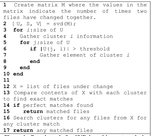
Our technique provides a methodology that derives associations using SVD based upon a set of change records from testing and field failures. These association clusters of files portray an underlying structure in the system indicating how files tend to be executed, tested, and changed together. We decided to use SVD in our methodology to leverage its ability to illuminate underlying structures in a data set in which the data could be associated in multiple ways. In this section, we will describe our technique, which includes deriving the association clusters from change records and interpreting the results of the analysis. An outline of our technique can be found in Figure 1.
3.1 Identifying data sources
Source control systems are the primary source for gathering change records. When a developer checks a file in to a source control system, the system typically records the time of the check-in along with information about the developer and the nature of the change. Individual changes can be often be linked together into tracks, either through a specific mechanism in the source control system that records that information or through the examination of change record check-in information. With information regarding tracks, we are able to ascertain how files change together.
Some more complex source control systems are also integrated with a fault tracking system. With these more complex systems, tracks can be associated directly with the fault record that the changes are addressing, providing detail about how tracks are linked together. Information from fault tracking systems allows us to isolate tracks to those made under specific circumstances. For example, changes derived from faults found during system test could be compared to changes derived from field failures discovered by customers.
3.2 Mining software development artifact data
After appropriate data sources have been identified, an analysis matrix should be generated that contains the system’s files along each axis. The values within the analysis matrix show how the files are connected through change records. For illustrative purposes on how to build the analysis matrix, we will use a set of sample data to generate this analysis matrix. Table 1 shows a small sample of the set of the change records that were used to 1 Create matrix M where the values in the matrix indicate the number of times two files have changed together.2 [U, S, V] = svd(M);
3 for i:size of U
4 Gather cluster i information
5 for j:size of U
6 if |U(j, i)| > threshold
7 Gather element of cluster i 8 end
9 end 10 end 11
12 X = list of files under change
13 Compare contents of X with each cluster to find exact matches
14 if perfect matches found
15 return matched files
16 Search clusters for any files from X for any cluster match
17 return any matched files
create our example analysis matrix. This example uses a small system consisting of five files.
Table 1. Sample Change Record Information. Test Case
ID
Fault ID Track ID Files
Changed
T1 A1 988 1
T2 A2 989 2, 3
T3 B1 990 4, 5
T3 B2 991 4, 5
T1 B3 992 1, 2
T4 C1 993 2, 3
We have built an example analysis matrix M, shown below in Equation 1 using the data from Table 1 and additional change records. The values in the matrix represent the number of times that each file appeared in a track with another file. Thus, File 2 has appeared in a track 10 times together with File 1, 21 times together with File 3, and 0 times by itself (since M(2,2) = M(2,1) +
M(2,3)). Similarly, File 3 has changed 21 times with File
2 and 3 times by itself.
! ! ! ! ! ! " # $ $ $ $ $ $ % & = 17 12 0 0 0 12 15 0 0 0 0 0 24 21 0 0 0 21 31 10 0 0 0 10 25 5 4 3 2 1 5 4 3 2 1 F F F F F M F F F F F (1)
Upon initial examination of this matrix, we note that Files 4 and 5 change together or by themselves. Based on this, it appears that Files 4 and 5 are strongly linked in isolation from the rest of the system. Similarly, Files 1, 2, and 3 are also linked, with Files 2 and 3 having the strongest bond of the three.
3.3 Perform the singular value decomposition
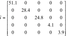
To determine the strength of the associations between files and to generate the association clusters, we perform a SVD of this matrix. The strength of the association is determined by the frequency of time the files changed together. A SVD of M provides the following matrices, shown in Equations 2 and 3:! ! ! ! ! ! " # $ $ $ $ $ $ % & ' ' ' ' ' ' ' ' ' = = 68 . 0 0 74 . 0 74 . 0 0 68 . 0 0 69 . 43 . 0 59 . 0 56 . 02 . 0 76 . 0 31 . 9 . 0 29 . V U (2) ! ! ! ! ! ! " # $ $ $ $ $ $ % & = 9 . 3 0 0 0 0 0 1 . 4 0 0 0 0 0 8 . 24 0 0 0 0 0 4 . 28 0 0 0 0 0 1 . 51 S (3)
The U and V matrices provide information as to the structure of the association clusters. The singular values from the S matrix represent the amount of variability each association cluster contributes to the original analysis matrix. Note that U and V are equal, due to M being a symmetric matrix.
A cluster’s strength, represented by the size of the singular value coupled with it, indicates the amount of variability that the association cluster provides to the original analysis matrix [20]. Dividing a cluster’s singular value by the sum of all the singular values provides the percentage of how representative the cluster is of the original matrix. In this example, a high singular value indicates that that association cluster is more prominent in the analysis matrix, due to a greater number of changes that have occurred to that set of files. A high singular value could be indicative of a particularly problematic section of code or a new feature that has just been introduced into the system and is experiencing its first rigorous testing.
3.4 Gather the association clusters
The values in the U matrix correspond to the composition of each association cluster. In this example, there are five association clusters because the rank of M is five. The first column of U, representing the structure of the first association cluster, is coupled with the first singular value in S, representing the strength of that association cluster. Since it is coupled with the largest singular value, the first association cluster represents the greatest amount of variability in the original analysis matrix and is the most prominent association cluster. From the U matrix, we see that the first association cluster is comprised of Files 1, 2, and 3, indicated by the fact that the three files all have values with a similar sign. Further, each of these values has a larger magnitude than .1, the threshold we used in our research. A threshold is used when selecting cluster members so that only files with a strong association to the other files are included in the cluster. This is similar to the threshold that Osinski used in his algorithm [16]. In the third cluster, we see that File 1 is its own cluster that can, at times, change without Files 2 and 3. So, in effect, we get two associations out of the third cluster, one with File 1 by itself and one with Files 2 and 3 together.
weighted within that association cluster as to its degree of participation. For example, the first association cluster is primarily composed of File 2 and File 3 due to their higher values. File 1 is a minor participant in this association cluster. If we reexamine the original analysis matrix M, we can see the strong correlation between Files 2 and 3 with a somewhat looser correlation with File 1, since these files only tend to change together and not at all with Files 4 and 5. The association cluster in the second column portrays the next most significant cluster, comprised of Files 4 and 5.
The singular values of these clusters found in the S matrix provide some indication as to how they should be analyzed. The first cluster represents 45% of the overall variability in the matrix, which can be determined by dividing the first singular value by the sum of all the singular values. Further, the third cluster represents 22% and the fourth represents 4%. These percentages show that the first cluster defines the majority of the information regarding these files. Clusters three and four are, in effect, sub-clusters of the first cluster because they contain a similar set of files. At this step in our technique, the matrix U can provide information about the likelihood of a change in an association cluster based upon previous change information.
Using the U and S matrices generated from our technique, we can determine the possible impact that a new track might have on the system. We can compare the associations gathered from the U matrix with a new track. If all the files in a new track are present in a previously- determined association cluster, we know that there is a strong relationship between the changed files and the other files in the cluster and that these files would be the most likely files to be affected by this change. Further, the magnitude of the corresponding singular value in S indicates which cluster has churned more within the data set under examination. If the files in a new track do not all appear in the same cluster, then they represent a new execution path through the system. In this instance, files that are associated with each changed file separately can possibly be affected by this change. Finally, the files may have never changed before within the data set that was used to build the U matrix. In this instance, no historical evidence exists as to how these files may affect the system, and a new association cluster is will form to represent this new set of changes in a future analysis.
This technique is similar to the cluster rank algorithm used by Osinski et al. in their SVD-based search term clustering algorithm [16]. Osinski multiplied their document matrix by a modified U matrix from the SVD to derive the impact that each search term had on a given document. In this fashion, the values from the result vector were used to assign a document to its closest-matching search term cluster [16].
3.5 Limitations
The association clusters are based upon the change records that may or may not be accurate. For example, the case study reported in this paper uses data from an IBM system. IBM’s documented development process and interviews from developers and managers indicated that files that were changed together are related and are addressing a specific fault. The process in place in IBM helps to minimize opportunistic changes whereby a developer makes changes unrelated to an open fault while fixing that fault. If opportunistic changes occur during fault removal efforts, we cannot be certain that the set of files that change together are related to a particular fault. Conversely, opportunistic changes and aggregating multiple changes in one change record may be prevalent in open source projects
Another limitation is that our technique is not guaranteed to be safe. If there is no historical data regarding a set of files, our technique cannot provide guidance as to where the effects may be. However, our technique may be more practical for a system with a large percentage of non-executable files. Dynamic techniques might not be able to find the same dependencies that our technique finds among these files since dynamic techniques operate primarily on source files.
Current impact analysis techniques typically calculate the impact of a proposed change at the function or line of code level, while our technique is currently being used at the file level. Using a technique that has a granularity level down to a line of code can be beneficial if a source file is large in size, since a line of code granularity would limit the area that a developer would have to analyze to find the affected code. However, since our technique is also focusing on non-executable parts of the system, the file level is the most effective granularity level for our purposes. In most cases, change information does not exist to the line level of some non-executable files, such as help files. Further, the file level is effectively the only appropriate granularity for media files that are included in a system.
4. IBM Case Study
4.1 Case study setup
We began by examining available data sources. IBM’s source control and fault management system generates detailed logs on tracks. The project that was selected had three consecutive minor releases. Each release of the project contained approximately 21,000 files with over one million lines of code. To protect proprietary information, we cannot provide the quantity of change records analyzed in this paper.
4.2 Cluster identification
Our first research question was to determine if the association clusters produced by SVD are intuitively identifiable by system experts and thus represent actual system components. Beyer and Noack [3] evaluated their clustering algorithms based upon how accurately the clusters represented sub-systems compared to an actual decomposition of the system. Osinski et al. [16] performed a comparable exercise using multiple sets of documents and interviewing users on whether the search results from the algorithm were useful. We followed a parallel approach to previous research to qualitatively assess the accuracy of the clustering algorithm.
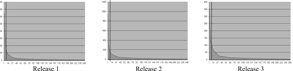
Once we generated the association clusters for the three releases, two authorities on the system, a testing manager and a senior technical staff member, were independently shown the sets of files that comprise the clusters with the highest singular values. The authorities were asked to give each cluster a name based upon the types of files in the cluster (e.g. system configuration files). This naming step is not a required step in our technique, however, it aids us in answering the research question For the purposes of this cluster identification exercise only, we limited the number of clusters for analysis to the first six for each release (18 total), which accounted for approximately 25% of the overall variability in the original matrix. The first six in each release were chosen for this case study because, after the sixth singular value, the singular values drop off significantly and slowly
reduce to zero as shown in Figure 2. Thus, we selected the most prominent clusters for our identification analysis in this case study. Graphs of the top 250 singular values for each release are shown Figure 2. The top 250 are shown because the full graph of all 21,000 singular values is difficult to interpret visually.
The two authorities on the system independently provided similar names for each cluster. The identifications and singular values for the six association clusters for each minor release are shown in Table 2 and are in order by singular value. Further, the main release requirements for all three releases were evidenced in the top six association clusters, indicating that the association clusters can identify system components and order them by velocity of change as indicated by the magnitude of the singular values. Another thing to note about these clusters is approximately 83% of these clusters include files that are not source code, including license files, help files, configuration files, and images from the graphical user interface. This result indicates the importance of non-executable files in this particular project.
Release 1
Release 2
Release 3
Figure 2. Graphs of top 250 singular values for the three minor releases.
Table 2. Results from association cluster creation. Assoc.
Cluster Release 1 Release 2 Release 3
1 Patch config
files
Release req. 2.1 Release req. 3.1
2 System config
files
Database Release req.
3.2
3 Database System config
files
Graphical user interface
4 Patch
information Release req. 2.2 Source control files
5 Release req.
1.1 License files Release req. 3.3
6 License files Graphical user
4.3 Impact analysis investigation
We addressed our second research question “Do the association clusters produced by SVD accurately surface sets of files that are indirectly impacted by a system modification?” in two stages. We first wanted to determine the size of the impact sets returned by our technique, and then we investigated the accuracy of those impact sets. First, we measured the size of the impact sets generated by our technique to determine how much our technique minimized the impact set. We used a random data splitting technique with the three minor releases of an industrial software system in this investigation to create our data sets. We began by randomly selecting two-thirds of the tracks for each release as the “historical data” from which we generated a set of association clusters. The remaining one-third of the tracks were then used as our “future set,” which would simulate incoming tracks made to perform a system modification. We performed this data splitting exercise ten separate times for each release.
The impact analysis techniques used by Orso et al. [14] and Law and Rothermel [11] are considered safe. As a result, these researchers showed the efficacy of their impact analysis technique by comparing the size of the impact set against that of other impact analysis techniques. We utilized a similar methodology to first investigate the relative reduction of the impact set.
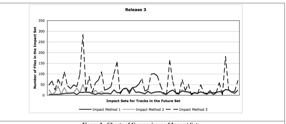
We gathered impact sets from the system modification in the future set using three different impact methods: two using our algorithm found in Figure 1 (Impact Methods 1 and 2) and another as a baseline (Impact Method 3):
• Impact Method 1: gather all the files that appear in clusters in which all of the newly-changed files appear (for example, if a new track contains files A, C, and Q, a file is considered in the impact set if
it appears in a cluster in which A, C, and Q all appear together)
• Impact Method 2: gather all the files that appear in clusters in which any of the newly-changed files appear (for example, if a new track contains files A, C, and Q, a file is considered in the impact set if it appears in any cluster that contains at least one of files A, C, or Q)
• Impact Method 3: gather all the files that have changed in the “historical data” with any of the newly-changed files (for example, if a new track contains files A, C, and Q, a file is considered part of the impact set if that file has been modified in conjunction with either A, C, or Q in a system modification in the historical data)
We compared the size of Impact Methods 1 and 2 impact sets to that derived by Impact Method 3. The goal of this comparison is to show that using SVD can narrow the scope of files that should be examined in the event of a system modification to those files that are most strongly connected to the changing files. An example result from Release 3 can be found in Figure 3.
All three releases followed a similar pattern to the result shown from Release 3 in Figure 3. The lines in the chart represent the quantity of impacted files for each track found in the future set. The chart shows that the size of the impact set is generally significantly reduced using either Impact Methods 1 or 2 that utilize the association clusters. Further, the size of the impact set remained relatively constant, despite spikes in the size of Impact Method 3. This relative constant size is an indication that the general size of clusters is relatively the same, allowing for a more targeted impact analysis.
After we evaluated the reduction of the size of the impact set using our technique, we investigated the accuracy of those impact sets. Because our technique
generates an impact set based upon historical evidence, the files in the impact set could be considered as a recommendation for further inspection of additional files. Thus, we evaluated the accuracy of the Impact Method 1 by determining whether the files in the impact set appeared in the future set along with one of the files from the new system modification.
For our the discussion of our accuracy analysis technique, consider a track in the future set that contains files A, B, and C. Impact Method 1 generates a cluster that contains A, B, C, and D, thereby providing a recommendation that D also be examined. We refer to files A, B, and C as files in the “test track” and to file D as a file in the “impact set.”
For our analysis, we considered a file in the impact set a confirmed true positive if that file appeared in any track in the future set with one or of the files from the test track. For example, if D appears in a track in the future set with either A, B, or C, we consider this matching result as a confirmed true positive. However, if D does not appear with A, B, or C in the future set, the conditions of system activity may simply not have involved these files. Thus, any recommendation that is not a confirmed true positive may either be an unconfirmed true positive or a false positive.
We performed this investigation of Impact Method 1 within each of the three minor releases. We also used the results of Release 1 with the changes from Release 2, and the results of Release 1 and 2 with the changes from Release 3. In an industrial setting, the association clusters adjust as new change records are gathered when new features or faults are discovered. The technique evolves along with the system itself. The results of this investigation can be found in Table 3.
Note that between 21.1% and 55.3% of the files that were indicated as impacted in any given system modification were non-source files and would not have been considered in current semantic impact analysis techniques. This is partly the result of the type of system under investigation in this case study, but the results do indicate that often non-source files, such as images or help files, can be impacted by a system modification. Also note that the average number of impacted files is in addition to the actual changed files in the system modification.
We discovered that the accuracy of our technique is
correlated with the quantity of the number of changes for a set of files under change. For example, in Release 1 and Release 3, there were a small number of areas of the system that were under change. The files in these areas had a relatively large number of changes associated with each of them. However, in Release 2, even though there were a larger number of changes overall, the changes were spread out evenly across the system. The SVD creates associations based upon the velocity of change, so areas with a higher change density cluster together better than larger areas with a lower density. What this lower change density yields is a larger impact set because the SVD associates more files together, as is the case in Release 2. However, with enough information about how files change together with when the changes from Release 2 were combined with those from Release 1, the confirmed true positive rate improved because the overall change density increased.
In our background research for this work, we did not discover any other empirical analysis of an impact analysis technique that examined the accuracy of the technique based upon future system modifications. Other techniques were validated by examining the size of the impact set, given that the technique was considered safe.
5. Summary and Future Work
In this paper, we propose an empirically-based impact analysis methodology based upon structures discovered through change records and singular value decomposition. Our technique makes use of the information in change records to discover and define relationships between files within the system. The novel aspect of our technique as compared to other impact analysis techniques is the use of change records to drive an impact analysis that requires no access to the source code itself and also can incorporate all files in a system, even source files. In some systems, faults in non-source files can be just as severe as those in the code base [10]. Further, our technique utilizes historical evidence as to areas of the system currently under change to highlight files that are most likely to change together.
To examine the efficacy of our technique, a post hoc case study was performed with three releases of a product from IBM. The generated association clusters from the analysis were identifiable and directly relatable to specific
Table 3. Investigation results.
Release Confirmed True Positive Rate % Non-Source Files Avg./Med. Track
Size
Avg./Med. Size of
Impact Set
1 45.4% 35.2% 19.3 / 3 21.1 / 3
2 10.0% 55.3% 40.5 / 4 43.9 / 5
3 39.5% 34.4% 22.4 / 3 21.2 / 3
1 w/ 2 31.5% 21.1% 28.3 / 4 24.4 / 3
requirements for each release or for an identified internal system component. The association clusters specifically illuminated areas of the code base where cross-component dependencies existed and cross-components that included files that would not normally be examined in an analysis that used execution-based files, such as help files and configuration files. With enough information about how files change together, our technique has a confirmed true positive rate of around 40%. The other files in the impact set that are not confirmed true positives are either unconfirmed true positives or false positives.
Our primary goal in future work is to do a comparison with our technique and a dynamic impact analysis technique, such as CoverageImpact. We are interested to see if the results of an execution-based impact analysis match how files tend to change together. An investigation into this comparison could indicate that files that change together are often related in execution. We would also like to investigate further the importance of non-executable files in an impact analysis. There also may be a way to combine our technique with a dynamic impact analysis technique. If we substituted files that call each other (as shown in a call graph) for files that change together, we would have a hybrid technique that utilized dynamic information with the SVD technique.
6. Acknowledgments
We would sincerely like to thank J.B. Baker at IBM for his input into this work. We would also like to thank the Realsearch reading group for critiquing early versions of this research. Partial funding was provided for NCSU authors by the National Science Foundation.
7. References
[1] Arnold, R. and Bohner, S., "Impact Analysis - Towards A Framework for Comparison," Conference on Software Maintenance, Montreal, Canada, 1993.
[2] Ball, T., Kim, J., Potter, A., and Siy, H., "If your version control system could talk," Workshop on Process Modeling and Empirical Studies of Software Engineering, 1997. [3] Beyer, D. and Noack, A., "Clustering Software Artifacts Based on Frequent Common Changes," 13th IEEE International Workshop on Program Comprehension, St. Louis, MO, 2005.
[4] Bohner, S., ""A Graph Traceability Approach to Software Change Impact Analysis"," in Department of Computer Science, vol. PhD. Fairfax, VA: George Mason University, 1995.
[5] Canfora, G. and Cerulo, L., "Impact Analysis by Mining Software and Change Request Repositories," International Software Metrics Symposium, 2005.
[6] Demmel, J., Applied Numerical Linear Algebra.
Philadelphia: Society for Industrial and Applied Mathematics, 1997.
[7] Gall, H., Jazayeri, M., and Krajewski, J., "CVS Release History Data for Detecting Logical Couplings," Sixth International Workshop on Principles of Software Evolution, 2003.
[8] Hoffman, T., "Probabilistic Latent Semantic
Analysis," Conference on Uncertainty in Artificial Intelligence, Stockholm, Sweden, 1999.
[9] Huang, L. and Song, Y.-T., "Dynamic Impact Analysis Using Execution Profile Tracing," International Conference on Software Engineering Research, Management, and Applications, 2006.
[10] Jalote, P., Software Project Management in Practice. New York: Addison Wesley Professional, 2002.
[11] Law, J. and Rothermel, G., "Whole Program Path-Based Dynamic Impact Analysis," International Conference on Software Engineering, Portland, OR, 2003.
[12] Livshits, B. and Zimmermann, T., "DynaMine: Finding Common Error Patterns by Mining Software Revision Histories," European Software Engineering Conference and Symposion on the Foundations on Software Engineering, Lisbon, Portugal, 2005.
[13] Maletic, J. I. and Marcus, A., "Using Latent Semantic Analysis to Identify Similarities in Source Code to Support Program Understanding," 12th IEEE International Conference on Tools with Artificial Intelligence, Vancouver, British Columbia, 2000.
[14] Orso, A., Apiwattanapong, T., and Harrold, M. J., "Leveraging field data for impact analysis and regression testing," Symposium on the Foundations of Software Engineering, Helsinki, Finland, 2003.
[15] Orso, A., Apiwattanapong, T., Law, J., Rothermel, G., and Harrold, M. J., "An Empirical Comparison of Dynamic Impact Analysis Algorithms," International Conference on Software Engineering, Scotland, 2004.
[16] Osinski, S., Stefanowski, J., and Weiss, D., "Lingo: Search Results Clustering Algorithm Based on Singular Value Decomposition," Advances in Soft Computing, Intelligent Information Processing and Web Mining, Zakopane, Poland, 2004.
[17] Ren, X., Shah, F., Tip, F., Ryder, B., and Chesley, O., "Chianti: a tool for change impact analysis of Java programs," Conference on Object-Oriented Programming, Systems, Languages, and Applications, Vancouver, Canada, 2004. [18] Tip, F., "A survey of program slicing tecniques,"
Journal of Programming Languages, vol. 3, pp. 121-189, 1995. [19] von Knethen, A. and Grund, M., "QuaTrace: A Tool Environment for (Semi-) Automatic Impact Analysis Based on Traces," International Conference on Software Maintenance, 2003.
[20] Will, T., "Introduction to the Singular Value Decomposition," vol. 2006: UW-La Crosse, 1999.
[21] Ying, A., Murphy, G., Ng, R., and Chu-Carroll, M., "Prediction Source Code Changes by Mining Change History,"
IEEE Transactions on Software Engineering, vol. 30, pp. 574-586, 2004.