ABSTRACT
POOSAMANI, NITHYANANTHAN. Enabling Accurate and Energy-Efficient Context-Aware Systems for Smart Objects using Cellular Signals. (Under the direction of Dr. Injong Rhee.)
The Internet of Things (IoT) paradigm aims to interconnect a variety of heterogeneous Smart Objects (e.g., sensors, smart devices, home automation equipment) using Machine-to-Machine communications. Smart devices have become one of the primary ways for people to access entertainment and other business applications, both inside and outside of their homes. This has led to two significant problems: substantial increase in monthly wireless data usage, and a rapid drain in smart phone battery life. Another recent trend with small form-factors in devices has lead to a bulk of the device components fused together using adhesives without being exposed to outside world (e.g., battery is glued to panel case or screen without exposing the circuit terminals). This prevents researchers from measuring energy consumption ratings for the different sub-systems in the phone using power monitoring devices.
Smart devices that provide health monitoring, smart home and workplace, enterprise device management, and many others need to constantly sense their context and communicate with the network to collaborate with others. Mobile applications that provide location-specific services require either the absolute or logical location of users in indoor settings. Identifying the context of a user (e.g., in front of the store, suits section, billing counter, home, office, conference room) in a timely and energy-efficient manner is important for the applications to disburse appropriate deals or activate a set of device-specific policies. In all these cases, though sub-meter level accuracy is not required or expected, a practical and an infrastructure-independent solution which can be easily deployed in real world is highly preferred.
in mobile devices under different device screen activation scenarios and quantify the energy wastage due to unnecessary scan and association events under poor link conditions, which to the best of our knowledge has not been reported in previous literature. In our first work, iSha, we develop a fine-grained energy consumption analyzer system to estimate the energy consumption values of specific sub-components in smart devices which eliminates the need for specialized hardware power monitoring equipments.
In our second work, PRiSM, we develop a novel and light-weight signature matching system to automatically discover Wi-Fi hotspots without turning on the Wi-Fi interface in the smart device. It uses signal strengths received from cellular base stations to statistically predict the presence of Wi-Fi and connects directly to the hotspot without scanning. The system continuously learns based on user movement behaviours and auto-tunes its parameters accordingly. Hence, PRiSM, provides a practical and infrastructure-independent system to maximize Wi-Fi data offloading and simultaneously minimize Wi-Fi sensing costs.
In our final work, PILS, we develop a indoor localization system which logically maps the contextual information of the smart device with a specific indoor location using cellular multi-homing. We utilize a variety of back-channel parameters such as Received Signal Code Power (RSCP) from 3G radio cellular systems, Reference Signal Received Power (RSRP) and Reference Signal Received Quality (RSRQ) from 4G radio cellular systems in addition to Received Signal Strength (RSS) values from 2G radio cellular systems. We show the effects on location accuracy with using only connected base stations and with neighbouring base stations, self-sourced data and crowd-sourced data. We also show that by choosing a combination of signals from different cellular radio technologies specific to different locations provide better location accuracy than relying on one single radio technology for all indoor locations.
©Copyright 2015 by Nithyananthan Poosamani
Enabling Accurate and Energy-Efficient Context-Aware Systems for Smart Objects using Cellular Signals
by
Nithyananthan Poosamani
A dissertation submitted to the Graduate Faculty of North Carolina State University
in partial fulfillment of the requirements for the Degree of
Doctor of Philosophy
Computer Science
Raleigh, North Carolina
2015
APPROVED BY:
Dr. Mladen Vouk Dr. Rudra Dutta
Dr. Huaiyu Dai Dr. Injong Rhee
DEDICATION
BIOGRAPHY
ACKNOWLEDGEMENTS
I would like to first thank my advisor, Dr. Injong Rhee, without whose guidance, I would never have started on my doctoral program. He supported me through important stages of my research life. I would also like to thank the members of my dissertation committee, Dr. Mladen Vouk, Dr. Rudra Dutta and Dr. Huaiyu Dai for their kind help and patience. They had insightful questions and suggestions which helped me clarify my ideas and execute them. I am also extremely thankful for Dr. Khaled Harfoush and Dr. Mihail Sichitiu for suggestions and help during my doctoral examinations and for their feedback.
I would like to extend my sincere appreciation and thanks to all the staff members of Computer Science department for their help and support through these years. Special thanks to the Director of Graduate Program Dr. Douglas Reeves and Dr. George Rouskas. Special mention to administrative staff Ms. Kathy Luca, Ms. Linda Honeycutt, and Ms. Ann Hunt for their help and support through various day to day activities. I also like to thank Mr. Marhn Fullmer for assisting me with computer network related functions.
I would like to thank my colleagues with whom I had a wonderful opportunity to work with. Special thanks to Dr. Kyunghan Lee, Dr. Yaogong Wang, Dr. Sungro Yoon for their career and research related advice. I am also grateful to other lab members Jeongki Min, Arpit Gupta, Haiqing Jiang, Shuiqing Wang and SeungEun Chung for having shared precious moments in my doctoral study time. Special thanks to Shireesh Bhat for his help and support in crystallizing my thoughts and ideas. I also like to thank my mentors and advisors in both NetApp and Samsung Research for sharing their time and knowledge with me. Special mention to my mentors, Greg and Daniel from NetApp who helped me obtain a solid foundation for my industrial career.
The Campus Recreation at NC State. My first and only on-campus job was at the Carmichael Recreation center as an official and later as a Supervisor for recreational sports. Some of my best friends in the United States are from my memorable days at Campus Recreation. Thanks for taking me in to your family and showering with your warm southern culture. I will never forget the fun times be it the tailgating, or simple house parties. Thank you for making me one among you crazy bunch! I am gratified and humbled by my experiences with Maitri both as an Executive and as a student. My association with all the president’s I worked with brings back all the sweet memories. This section will not be able to hold the names of all the wonderful friends I made during my association with Maitri. Thank you all.
I would like to thank all my project coordinators and advisor’s in STARS for their encour-agement and support. Special thanks to Dr. Trisha Biswas, Veronica Catete and Robinson Udechukwu for putting up with me through thick and thin. Serving as the Treasurer in the executive body of UGSA for 2014-2015 opened my doors for financial accounting in huge organizations and to understand its nuances. It also helped me identify my abilities as an able administrator and engage for organizational success. Special thanks to my friends Bryan Hoynacke, Dr. David Fiala, Dr. Milena Bobea, Veronica Catete, Veronica Mbaneme, Chirag Gajjar, Katie Kennedy and Brooke Jordan for the awesome times in UGSA. Special mention to my advisors Dr. Barbi Honeycutt and Dr. Beth Overman and finance staff Ms. Ashley Chilton in helping me get through the job ever so easily.
experience the pleasure of public service when the transportation department made changes to the Centennial Route 10 after working closely with them for three years and will ever be cherished in my mind. Though there are innumerable people to personally thank, I shall keep it to my advisors who I interacted with the most and my personal well wishers: ‘‘Godmother” Ms. Eileen Coombes, Ms. Laura Stott, Ms. Deborah Felder, Ms. Allyson Clagett and Mr. Mike Giancola. You all made my five years of association with Student Government a wonderful memory. Special shout out to all my best friends I made during my time at SG.
Last but not least, an integral part of my life at NC State will be my association with The Office of International Services both as an orientation team member and as a student. Some of my friends for life were gifted to me here in OIS. Most of them are Ph.D. holders but I am going to address them as I normally would. Forgive my brevity! Lakshmi a.k.a. ‘‘Lauren Ball”, Ranjitha a.k.a. ‘‘Ranjith Kumar”, PP a.k.a. ‘‘PingPong Ganokon Urkasemsin”, jajaja a.k.a. ‘‘Jose”, Habibi a.k.a. ‘‘Ahmad”, Manjula a.k.a. ‘‘Manoj”, Joao a.k.a. ‘‘The Creepy Guy”, RT a.k.a. ‘‘Arthi Kannan”, and Saudi Prince a.k.a. ‘‘Tayseer”. The staff members here are more than just university employees and are a family to me. The best part is I get to talk with them more about my personal life than the regular student queries. My heartfelt appreciation and gratitude to all current and former members of the Office of International Services. Special shout out to Alexis, Kelia, Rebecca, Stacy, Mike, Thomas, Fernanda, Michael and Elizabeth!
Survival in a foreign country is not just knowing people but to feed yourself (literally!). I lost count of the number of times I ate food at my friends place. Vivake Ramasubramanian, Ramaswamy Adaikalavan, Balaji Soundararajan - I cannot thank enough for the wonderful support and love given by you and your family members. An important group of highly successful, talented and inspiring individuals who constantly motivate me are my school friends and their family: Adarsh, Ramu, Ganesen, Ashwin, Ajay. Thank you Supni, Kuppu, ‘‘stop-n-wait”, my undergraduate colleagues and numerous others for wishing me nothing but the best!
TABLE OF CONTENTS
LIST OF TABLES . . . xi
LIST OF FIGURES . . . xii
Chapter 1 Introduction . . . 1
1.1 Dissertation Roadmap . . . 3
Chapter 2 Background and Related Work . . . 4
2.1 Energy Measurements . . . 4
2.1.1 Screen Activation . . . 4
2.1.2 Sub-component Power . . . 4
2.2 Wi-Fi Sensing . . . 5
2.2.1 Wi-Fi Power Consumption and Reduction . . . 5
2.2.2 Wi-Fi Network Sensing . . . 5
2.2.3 Wi-Fi Data Offloading . . . 6
2.2.4 Wi-Fi Fingerprinting . . . 6
2.2.5 Smart Phone Usage pattern . . . 7
2.3 Indoor Positioning Techniques . . . 7
2.3.1 Infrastructure-based Approaches . . . 7
2.3.2 Fingerprinting-based Approaches . . . 8
2.3.3 Model-based Approaches . . . 8
2.3.4 Inertial Sensor-based Approaches . . . 9
2.3.5 FM-based Approaches . . . 9
2.3.6 GSM-based Approaches . . . 9
2.3.7 Localization Algorithms . . . 10
Chapter 3 iSha: A Fine-Grained Energy Analyzer System using Assembler and Disassembler . . . 12
3.1 Motivation . . . 14
3.2 Assembler and Disassembler . . . 15
3.3 System Design . . . 16
3.4 Evaluation . . . 17
3.4.1 Fine-grained Wi-Fi Energy Measurements . . . 17
3.4.2 Procedure to Compile Platform Source Code . . . 18
3.4.3 Procedure to Replace Supplicant Binary . . . 20
3.5 Discussion . . . 22
3.6 Concluding Remarks . . . 23
Chapter 4 PRiSM: Wi-Fi Hotspot Auto-Discovery System for Smart Objects 24 4.1 Motivation . . . 25
4.2.2 Cellular Signatures . . . 27
4.2.3 Existing Localization Algorithms . . . 32
4.2.4 Proposed Algorithm . . . 33
4.3 Implementation . . . 35
4.3.1 Architecture . . . 35
4.3.2 Operation . . . 36
4.3.3 Cost Analysis . . . 38
4.4 Evaluation . . . 38
4.4.1 Datasets . . . 39
4.4.2 Accuracy Measurements . . . 40
4.4.3 Energy Measurement Setup and Calculations . . . 44
4.4.4 Default Wi-Fi Vs. Footprint Vs. PRiSM . . . 45
4.4.5 Effect of Sensing Intervals (δ) and Wi-Fi Thresholds (τ) . . . 47
4.4.6 Overall Energy Impact . . . 49
4.4.7 Practical Verification of Energy Savings . . . 50
4.5 Discussion . . . 51
4.6 Concluding Remarks . . . 53
Chapter 5 PILS: A Context-Aware Indoor Positioning System via Cellular Multi-Homing . . . 54
5.1 Motivation . . . 55
5.2 Design . . . 56
5.2.1 Cellular Multi-Homing . . . 56
5.2.2 RSRP and RSRQ parameters . . . 61
5.2.3 Practical Algorithm . . . 61
5.3 Implementation . . . 64
5.3.1 Architecture . . . 64
5.3.2 Data Storage and Retrieval . . . 64
5.3.3 Cost Analysis . . . 66
5.4 Evaluation . . . 67
5.4.1 Datasets . . . 67
5.4.2 Accuracy Measurements . . . 67
5.4.3 Accuracy varies with number of base stations . . . 70
5.4.4 RSRP values provide better accuracy than RSS values . . . 73
5.4.5 RSRQ values provide less accuracy when used alone . . . 73
5.4.6 Radio network combinations increase accuracy . . . 76
5.4.7 Effect of accuracy on walking . . . 76
5.4.8 Effect of accuracy on room level detection . . . 76
5.5 Discussion . . . 79
5.6 Concluding Remarks . . . 80
Chapter 6 Conclusion . . . 82
6.1 Summary . . . 82
LIST OF TABLES
Table 3.1 Fine-grained energy measurements on Nexus One. . . 22
Table 4.1 PRiSM cellular signal sampling policy. . . 38
Table 4.2 Dataset information. . . 39
Table 4.3 Fine-grained measurements for Wi-Fi sensing. . . 45
Table 4.4 Total Wi-Fi usage and battery savings for users in dataset ‘D2’ for Wi-Fi offloading with τ = −80dBm. . . 49
Table 4.5 Nexus One practical energy evaluation. . . 51
Table 5.1 Energy consumption information per second between PILS and other ap-proaches used for continuous location sensing. . . 66
LIST OF FIGURES
Figure 3.1 Future is here: Internet-of-Things (image courtesy of theconnectivist.com). . 13 Figure 3.2 Architecture . . . 15 Figure 3.3 Repeated scan/association events under poor AP signal when the device
screen is (a) ON, (b) OFF. . . 18
Figure 4.1 Working of default Wi-Fi when (a) an AP is available to connect with, and (b) an AP is not available. . . 27 Figure 4.2 Repeated scan/association events under poor AP signal when the device
screen is (a) ON, (b) OFF. . . 28 Figure 4.3 Default Wi-Fi energy consumption for one minute under various screen
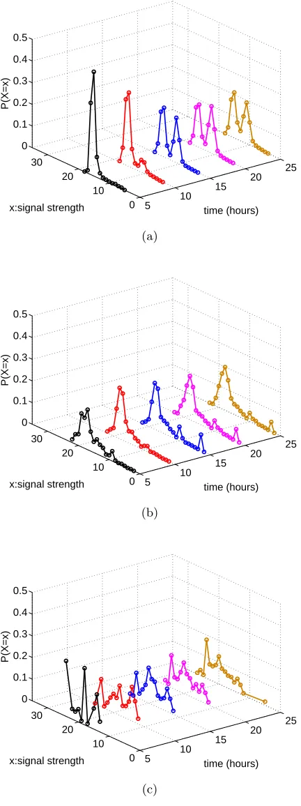
activation conditions. . . 28 Figure 4.4 The evolution of signal strength distributions from the most frequently
con-nected base station for 3 different APs are depicted in (a), (b), and (c). For each AP, the data is aggregated over time whenever connected with the AP. 29 Figure 4.5 The personalized signatures for three APs: (a) APX (b)APY, and (c) APZ.
The distance between APX and APY is about 7km,APY andAPZ is about
30meters. APY and APZ are located in the same building. The observed
base station IDs and their average signal strengths are given in the legend. . 31 Figure 4.6 PRiSM system architecture. . . 35 Figure 4.7 PRiSM operation includes three tasks: bootstrapping, signature matching,
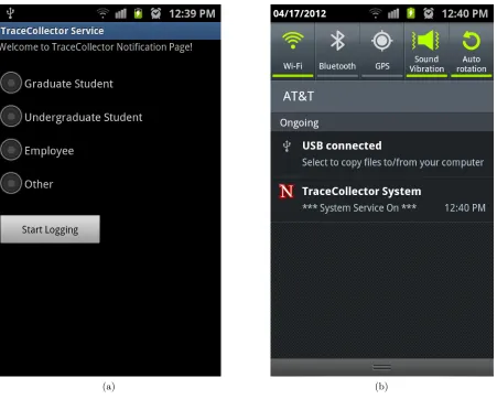
and online training. . . 36 Figure 4.8 (a) shows the launch screen of the service where user information is gathered,
(b) shows that the system service runs constantly in the background and logs all required information. . . 40 Figure 4.9 The number of hours logged by each individual user is shown during data
collection phase. . . 41 Figure 4.10 (a, b) ROC curves and (c)ρF P Vs.ρF N values for a randomly selected user
for all algorithms in dataset ‘D1’. ATiS achieves very high true positive and true negative values and very lowρF P and ρF N values simultaneously. . . . 42
Figure 4.11 (a) Average ρF P andρF N for users in dataset ‘D1’ and (b)ρF P and ρF N for
5 consecutive days for a user. . . 43 Figure 4.12 Monsoon Power Monitor setup connected with the phone. . . 44 Figure 4.13 Wi-Fi energy consumed every minute for (a) screen ON, (b) screen OFF, and
(c) under poor Wi-Fi signals. For Footprint, ∆1 is estimated to be 0.673mW h for screen on and ∆2 is estimated to be 0.719mW hfor screen off conditions. 46 Figure 4.14 Mean battery savings for all users in the dataset with 95 % confidence interval.
(a) vary δ givenτ =−80 dBm, (b) vary τ givenδ = 1 sec. . . 48
Figure 5.1 PILS signature element. . . 56 Figure 5.2 Cellular signal strength distribution of the mostly observed base stations at
Figure 5.3 (a) The number of observed base stations over time at a location. It fluctuates from 0 to 7. (b) The observed base station IDs over time.(c) CDF of the
number of observed base stations. . . 58
Figure 5.4 (a) Evolution of cellular signatures located at a location. . . 59
Figure 5.5 QQPlot of sample data Vs. Standard Normal values . . . 61
Figure 5.6 PILS system architecture. . . 64
Figure 5.7 PILS contextual signature storage database. . . 65
Figure 5.8 Office location layout. Cross marks represent the trial locations. . . 68
Figure 5.9 Home-SJ location. The different radio combinations are shown in different colored bars. The bars show average prediction probability and 95% confidence intervals error lines. . . 68
Figure 5.10 Prediction probability for various environments (a) Self-Sourced Data (b) Crowd-Sourced Data. . . 69
Figure 5.11 Prediction probability for various environments with special sorting techniques for BSSET and MSE(a) Self-Sourced Data (b) Crowd-Sourced Data. . . 71
Figure 5.12 Prediction error for various environments (a) Self-Sourced Data (b) Crowd-Sourced Data. . . 72
Figure 5.13 Prediction probability for change in number of observed neighbour BS (a) Home-SJ (b) Office. . . 74
Figure 5.14 Prediction probability for change in number of observed neighbour BS (a) University Room 1231 (b) Library. . . 75
Figure 5.15 Prediction probability for change in number of observed neighbour BS (a) University Room 1231 (b) Library. . . 77
Figure 5.16 Prediction probability for change in distance between adjoining test locations during hallway walk. . . 78
Chapter 1
Introduction
The Internet of Things (IoT) paradigm aims to interconnect a variety of heterogeneous Smart Objects (e.g., sensors, smart devices, home automation equipment) using Machine-to-Machine communications. A majority of consumer devices sold today come equipped with a variety of wireless communication technology (e.g., Bluetooth Low Energy, Wireless LAN, Near Field Communication, Cellular) to connect with the world-wide network.
With billions of such devices predicted to connect with the future internet, bringing the physical data from these devices to the digital world requires energy-efficient methodologies and standard communication protocols. Devices that provide health monitoring, smart home and workplace, enterprise data security, and many others need to constantly sense their context and communicate with the network to collaborate with others. A variety of the smart devices mentioned above are self-powered or connected to a power source glued to their components and hence the circuit terminals are not exposed to measure the energy consumption.
applications range from a simple calendar manager to complex business productivity software suites.
An ever increasing majority of these applications expect always-on internet connectivity (e.g., iCloud [5], other cloud-based services) so as to provide unlimited storage and processing capabilities. Dedicated cameras nowadays come with Wi-Fi interfaces. Smart devices have become one of the primary ways for people to access entertainment [6] (e.g., social networking, communication and browsing applications), both inside and outside of their homes. This has led to two significant problems: substantial increase in monthly data usage [7], and a rapid drain in smart phone battery life.
Smart devices have become one of the primary ways for people to access various business applications. Most of these applications provide location-specific services and hence, require either the absolute or logical location of users in indoor settings. Big retail giants and shop vendors in indoor locations such as malls, public convention center’s aim to provide specific deals and discounts to users who are within walking distance from their shops. Identifying the context of a user (e.g., in front of the store, suits section, billing counter) in a timely and practical manner is very important for the retail outlets to disburse appropriate deals.
Another fast developing trend is to selectively activate certain security features for smart devices in Enterprise Device Management (e.g., turn off camera inside office space, disable voice recorder in conference room). In the above applications, ‘front of the store’, ‘billing counter’, ‘conference room’ are few examples of logical locations or in the broad-sense referred to as the ‘context’ of the smart device. In all these cases, though sub-meter level accuracy is not required or expected, accuracy of the order of few feet (≈5 to 10f t) is highly preferred. However, to design a precise and an energy-efficient indoor localization system in an automated manner is (still) a very non-trivial task. The reasons include the need for: infrastructure-independent solutions, ease of practical deployment, and minimal battery consumption for users.
with minimal energy consumption, and context-aware indoor localization with minimal sensor costs. We propose iSha, PRiSM and PILS for those challenges and to prove the effectiveness of our solutions with working system prototypes and real data traces.
1.1
Dissertation Roadmap
The rest of this organized as follows:
Chapter 2 provides the background information and also provides description about the previous works related to the different topics under consideration.
Chapter 3 provides information about the system and implementation of a fine-grained light-weight energy analyser system, iSha. The system uses a OS-independent solution using smali/backsmali, a assembler/disassembler module functionality described in Chapter 3.2. The system design is presented in Chapter 3.3. Discussion about possible future work is given in Chapter 3.5. Concluding remarks for this topic is presented in Chapter 3.6.
Chapter 4 describes PRiSM, a Wi-Fi hotspot auto-discovery system. It discusses the various components of system design in Chapter 4.2 and the real-world system implementation is Chapter 4.3. Simulation results based on real world traces and practical verification of energy savings are discussed in Chapter 4.4. Concluding remarks for this topic is presented in Chapter 4.6. Chapter 5 provides information about a context-aware indoor localization system called PILS using the technique of cellular multi-homing. Details about cellular multi-homing and the suitability of cellular signals for such indoor location matching systems are discussed in Chapter 5.2. The prototype system implementation is described in Chapter 5.3. The performance measurements are discussed in Chapter 5.4 and possible drawbacks and future optimizations are provided in Chapter 5.5. Concluding remarks for this topic is presented in Chapter 5.6.
Chapter 2
Background and Related Work
This chapter provides the background and existing research in the areas pertaining to our dissertation: energy measurements, Wi-Fi sensing related mechanisms, and indoor localization techniques.
2.1
Energy Measurements
2.1.1 Screen Activation
Huge energy savings are reported for power measurements for cellular radio/LTE traffic obtained during screen-off conditions [8], Wi-Fi [9--12]. However, we perform measurements under both screen on and off conditions, show that screen off energy is more compared to screen on due to use of CPU wakelocks, and use appropriate energy values for user logs. Hence, the final energy figures in our experiments more accurately match actual Wi-Fi power consumptions.
2.1.2 Sub-component Power
measurements, there following are a few works which directly relate to measuring the energy consumption in mobile or smart devices: [13, 14]. Since these works do not take in to account the recent OS changes and the power dynamics associated with latest integrated Circuit chips, they do not account for the dynamic power variations in smart devices. These works assumed a constant baseline-power level for mobile devices and calculated the excess power consumption to other operating components. They also only allow for small range of variations. iSha [15, 16] differs from the previous works in that it dynamically modifies the executable code and inserts specific log-triggers to achieve fine-grained energy measurements.
2.2
Wi-Fi Sensing
2.2.1 Wi-Fi Power Consumption and Reduction
Wi-Fi power consumption has been studied in previous works: TailEnder [11], [12]. The measure-ments were done on Android G1 (0.175mW h) and Nokia N95 (1.4mW h[11], 0.328mW h[12]) mobile phones. Our measurements on Android Nexus One show comparatively less values as shown in Table 4.3. Wi-Fi has high initial cost for scan/association [11]. Many techniques are proposed to mitigate the excessive power consumption by Wi-Fi radios. Wake-on-Wireless [17] and E-Mili [18] reduce the idle state power consumption of Wi-Fi by installing a secondary low-power transceiver for idle listening and by down-clocking the Wi-Fi chipset during idle periods respectively. Recently, NAPman [19], SleepWell [20] proposed intelligent idle period reduction schemes to enable Wi-Fi to stay in the PSM mode longer than usual. We try to reduce Wi-Fi sensing costs (radio power up/down, scan, association and DHCP) and do not focus on power consumption during idle periods or during data transfer.
2.2.2 Wi-Fi Network Sensing
The algorithms consider information such as AP inter-arrival time, AP density and user velocity. These algorithms either increase/decrease Wi-Fi sensing intervals upon failure to meet APs and hence will not work well for all users because the Wi-Fi connectivity and movement patterns of users differ significantly.
Some other works determine the Wi-Fi sensing policy using on-the-board sensors in smart phones (e.g., Accelerometers [9], GPS [22--24], Bluetooth [25]) or off-the-board sensors (e.g., Zigbee [26]). However collecting information from those sensors pose additional energy overhead (e.g., Accelerometers consume close to 0.667mW hevery 30sec[27]) and some resources may not be available always (e.g., GPS is not available indoors, availability of Bluetooth users). We utilize readily available GSM cellular signals at zero extra energy cost and predicts AP availability without the aid of alternative sensor information.
2.2.3 Wi-Fi Data Offloading
Prior research works quantify the efficiency of mobile data offloading through available Wi-Fi networks. [28] predicts future Wi-Fi throughput and waits to delay data transfer only if the 3G savings expected are within the application’s delay tolerance. [29] shows that over 70% of data can be offloaded if delayed by two hours. [12] selects 3G or Wi-Fi links to transfer data based on the Lyapunov optimization framework to minimize energy expenditure. PRiSM [30, 31] on the other hand does not provide quantitative bounds on the amount of data that can be offloaded or decides between Wi-Fi and 3G, instead, we try to maximize such offloading opportunities with minimal energy consumption.
2.2.4 Wi-Fi Fingerprinting
distribution and hence takes a non-parametric approach.
Few other works use multi-modal sensors (e.g., Accelerometers [9], GPS [22--24], Blue-tooth [25], Zigbee [26]) in addition to identify context. Unlike PRiSM, the sensors may not be available always and they consume extra battery energy (e.g., Accelerometers consume close to 0.667mW hevery 30sec [27]). Some require infrastructural changes and extensive war-driving efforts to obtain feature-rich data sets. Also, most commercial systems (e.g., WiFi Sense [34], Place Lab [35]) turn on the radio interfaces continuously to identify context which results in battery drain.
2.2.5 Smart Phone Usage pattern
The usage pattern of smart phones differs on an individual basis. [6] characterizes the user interaction with the device and the variety of applications used and the impact of those activities on network and energy usage. [36] provides the network performance experienced by the users solely when they are interacting with their devices. It also argues how poor network performance results in a bad user experience.
2.3
Indoor Positioning Techniques
2.3.1 Infrastructure-based Approaches
phones.
2.3.2 Fingerprinting-based Approaches
The most widely used approach for mapping RF signals to location uses received signal strength (RSS). Here a signal map of RSS fingerprints is constructed for every location. This RSS fingerprint was introduced by RADAR [32] and it constructed Wi-Fi signal maps at locations from one or more access points, achieving accuracies of the order of a few meters. Later systems such as Horus [33] used probabilistic techniques to improve accuracy. However, the above systems had extensive calibration overhead.
A recent approach [43] tried to reduce calibration and increase accuracy further using statistical modeling of signal strengths. Thus in general, fingerprinting-based approaches consume considerable time and effort to generate the signals maps of the locations. Moreover, current state-of-art techniques utilize Wi-Fi signals for indoor localization which are prone to multi-path and fading effects from static objects and human movement. A recent work [44] proposed using OFDM PHY layer information for more robust performance but still requires extensive signal logging and hence depletes battery energy quickly. PILS [42] uses cellular signals already received by smart phones at no extra-cost and runs in the background collecting signals for the places visited by the user. Also, we try to reduce the dependency on RSS signals by utilizing other network-related signals (e.g., Received Signal Reference Power, Timing Advance).
2.3.3 Model-based Approaches
compute the required database. Our work [30, 42], on the other hand, stores cellular signals in a novel way within the user‘s phone and reduces computation complexity.
2.3.4 Inertial Sensor-based Approaches
Current smart devices in the market come with a variety of sensors such as accelerometer, gyroscope, barometer, and magnetometer. In these cases, if the starting location is known, the user can be tracked in indoor settings. Accelerometer signals have been used along with dead-reckoning to provide indoor pedestrian localization [51, 52]. A mixture of sensors have been utilized to synthesize unique signatures for different locations [53]. All these multi-modal sensing techniques still require other radio signals (e.g., Wi-Fi, cellular) to increase the accuracy and continuous running of these sensors pose extra energy overhead for the battery.
2.3.5 FM-based Approaches
The operating frequency range of Wi-Fi signals makes it sensitive to static objects and human movement due to multi-path and fading. To overcome these limitations in indoor settings, few research works utilized FM signals for localization [54, 55]. FM signals are shown to experience less temporal variations when compared to Wi-Fi signals in indoors and hence provide good location accuracy. However, the explicit need to know the location of FM stations and floor plans to generate FM signal maps and the need for large windows in the building [55] make these techniques not feasible for practical deployment.
2.3.6 GSM-based Approaches
100−150meter accuracy. Though the volume of research is huge in indoor localization, not many works have utilized GSM signals. Our work, PILS [42] is very different from above previous works in that it utilizes the statistical properties of the entire spectrum of signals received from both connected and neighbor cells. It also does cellular multi-homing where GSM, UMTS and LTE signals are used to increase the accuracy of location prediction.
2.3.7 Localization Algorithms
A simple yet lightweight algorithm adopted for indoor and outdoor localization systems uses a set of base station IDs for matching (BSSET). In order to evaluate the likelihood of matching a fingerprint in the database, the algorithm can simply count the number of common BSs or can sum up the weight values of common BSs, where the weight is assigned to each BS based on its frequency of observation. Another class of algorithms use mean squared error (MSE) for matching [59, 60].
Most Artificial Intelligence (AI) techniques typically identify the topk fingerprints showing the smallest MSE values and then calculate the center from the locations paired with k fingerprints. This extension is called kN N (k-nearest neighbor) but they have the following problems: minimal training phase but costly testing phase including both time and memory, and assumes that data is in feature/metric space which means it is associated with some distance. Our work requires entire signal distribution clusters of the training data for quicker prediction and hence, uses a specialized hybrid algorithm to including lazy learning techniques and statistical algorithms from belief networks. Both BSSET and MSE algorithms need their own hard-coded threshold value (C) but PILS auto-tunes its threshold parameters regularly.
Chapter 3
iSha: A Fine-Grained Energy
Analyzer System using Assembler
and Disassembler
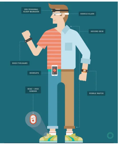
The Internet of Things (IoT) paradigm aims to interconnect a variety of heterogeneous Smart Objects (e.g., sensors, smart devices, home automation equipment) using Machine-to-Machine communications. A simple illustration of how these smart objects have become intertwined with our lives is shown in Figure 3.1. A majority of consumer devices sold today come equipped with a variety of wireless communication technology (e.g., Bluetooth Low Energy, Wireless LAN, Near Field Communication, Cellular) to connect with the world-wide network. With billions of such devices predicted to connect with the future internet, bringing the physical data from these devices to the digital world requires energy-efficient methodologies and standard communication protocols. Devices that provide health monitoring, smart home and workplace, enterprise data security, and many others need to constantly sense their context and communicate with the network to collaborate with others.
Figure 3.1: Future is here: Internet-of-Things (image courtesy of theconnectivist.com).
the energy consumption. It is also to be noted that the main components in these devices (e.g., Bluetooth, Wi-Fi, NFC) are mostly based on open-source implementations. Hence, it is easily possible to obtain the executable code running inside those devices at run-time.
system sub-components under different device screen states.
3.1
Motivation
The variability and complexity of hardware in smart devices has resulted in highly dynamic power variations as opposed to some existing power models with high baseline-power level and small dynamic range [13, 14]. So, the overall system power increasingly depends on highly granular sub-component power measurements. A majority of customer applications utilize Wi-Fi and Bluetooth, both of which have become integral components in most low-power wearable computing and smart devices. While new standards (e.g., 802.11ad) continuously emerge, it provides new opportunities for application and protocol developers to modify existing functionality and improve the user experience in these devices.
In very recent times, the popular mobile operating systems (e.g., Android [2], Apple iOS [3], Windows Phone OS [4], Blackberry OS [64], BADA [65]) have come up with specific Application Programming Interfaces (API) to show detailed statistics about power consumption by individual system components. However, there is a need to develop a universal approach to accurately measure energy consumption of certain device system components through real world usage patterns and not just under laboratory settings.
To that end, we need to develop a new light-weight system to analyze and model the energy consumption patterns of these technologies at a very fine-grained level and be simultaneously applicable for multiple devices. As a result, the developers can directly evaluate and optimize the energy efficiency of their protocols/methods without the need for a power monitor and also bring about energy savings to all applications which use them rather than profiling individual applications. Thus the question we ask ourselves is,‘‘Can we introduce a mobile OS-independent solution which can help researchers analyse energy consumption measurements in a variety of
Figure 3.2: Architecture
3.2
Assembler and Disassembler
An assembler is a utility program used to convert the syntax for operations in a programming language and the mnemonics in to the object code suitable for the hardware to run. A disassembler is a computer program to translate the machine language back in to the assembly language. This operation is the inverse of what the assembler does. More information about assemblers and disassemblers can be found here [66, 67].
3.3
System Design
In this work, we develop a novel and light-weight system, iSha, to insert specific log triggers in the executable code using an assembler/disassembler module called smali/backsmali. The overall system architecture is shown in Figure 3.2. The system consists of three main processes: modifying the open source code of the internal phone component by the developer, modifying the runtime executable code inside the device dynamically using an assembler/disassembler module such as smali/backsmali, storing the energy measurement values and develop a energy model for future predictions. In these steps, it is assumed that the fine-grained energy measurements for individual sub-components in the phone or the device is available. The values can be published either by the manufacturer or a researcher who gets access to these measurement sheets or by way of manual measurement techniques.
3.4
Evaluation
In this section, we will discuss about our specific case study where we implemented iSha to deduce the fine-grained energy measurements if the Wi-Fi sub system and the measurement results obtained after multiple runs.
3.4.1 Fine-grained Wi-Fi Energy Measurements
In a smart phone, a Wi-Fi scan is initiated in response to two actions: by turning on the screen or when an application specifically requests for a scan. When an AP is available to connect, the Wi-Fi driver scans the available channels and connects to the pre-configured AP as shown in Figure 4.1 (a). If no such AP is found in the pre-configured list, it periodically scans until the device is successfully connected to an AP or until a connection time-out occurs in the Wi-Fi driver after 15 mins.
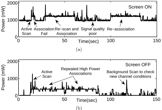
The default time interval for consecutive scans vary between 5-30 sec in various wpa -supplicant implementations. Upon screen off, the Wi-Fi radio chipset is turned off after a delay of 2 mins to avoid race conditions in the driver. CPU Wake locks are obtained for operations during screen off. While in connected state, if the link quality deteriorates, the Wi-Fi radio driver is kept in high power state constantly due to repeated scan and association requests. Also to avoid packet loss, the driver operates at lower modulation rates. Our measurements using a power monitor show the repeated scan/association operations in Figure 4.2. We start off by measuring the detailed power consumption patterns of Wi-Fi in mobile phones for different screen states (i.e., On, Off) under various Wi-Fi availability conditions (i.e., Good, Poor, Null) and data rates. The current power models do not consider such fine-grained variations, rather only consider the change in baseline power due to overall screen display brightness levels. Due to open source nature of Wi-Fi module (wpa supplicant) in Nexus One phones, we added logs in appropriate places to correlate the energy consumption with the specific system process.
0 50 100 150 0 1000 2000 Time(sec) Power (mW) Screen ON Active Scan Association Fail Re−scan and Association Signal quality poor Re−association (a)
0 50 100 150
0 1000 2000 Time(sec) Power (mW) Active Scan Screen OFF
Background Scan to check new channel conditions Repeated High Power
Associations
(b)
Figure 3.3: Repeated scan/association events under poor AP signal when the device screen is (a) ON, (b) OFF.
the baseline system power. Hence, it captures all the dynamic power variations in the process including tail energy for the series of chipsets. Using iSha, there is no need for developers to use physical power monitoring devices and can dynamically deduce the change in power consumption measurements.
3.4.2 Procedure to Compile Platform Source Code
In order to modify the Wi-Fi sub-component and replace the binary, the modified source code should be compiled within the entire platform source code for Android. In the section, we provide details to compile the platform source code of Android as follows. Some of the details for new Android OS releases may be different than that provided below.
• Set up Build Environment. Get Python installed.
• Install JDK 6 if you want to use Gingerbread or newer
– sudo add-apt-repository‘‘deb−src http://archive.canonical.com/ubuntulucidpartner”
– sudo apt-get update
– sudo apt-get install sun-java6-jdk
• Install all other required packages
• In this explanation, Linux version is Ubuntu 11.04. All following commands for ADB setup is for this version. For other lower versions, it may change. Test device is HTC Nexus One (Passion) running Linux kernel 2.6.32.x
• Get USB access to Linux System for using ADB (Android Debug Interface).
• Download Android source from git
– Make sure you have abin/directory in your home directory, and that it is included in your path.
∗ mkdir /bin
∗ P AT H = /bin:$P AT H
– Download the Repo script and ensure it is executable.
∗ curl https://android.git.kernel.org/repo > /bin/repo
∗ chmod a+x /bin/repo
– After installing Repo, set up your client to access the android source repository. Create an empty directory to hold your working files.
∗ mkdir W ORKIN G DIRECT ORY
∗ cd W ORKIN G DIRECT ORY
∗ repo init−u git://android.git.kernel.org/platf orm/manif est.git
– To pull down files to your working directory from the repositories as specified in the default manifest, runrepo sync.
– To compile the code after setting up all the environments including adb in your virtual machine, run the following in order.
∗ Run Nexus one script. Your phone should be connected with the virtual machine. · cd W ORKIN G DIRECT ORY
· cd ./device/htc/passion/
· ./extract−f iles.sh
∗ build the setting
· cd W ORKIN G DIRECT ORY
· repo sync −j16 · . build/envsetup.sh
· lunch f ull passion−userdebug
∗ To enable Debug Logs printed in wpa, change the log level toM SG DEBU G fromM SG IN F O at line 23 of the file wpadebug.c
∗ Now build it atW ORKIN G DIR. It takes around 2 hrs for initial build. · cd W ORKIN G DIRECT ORY
· make−j16
∗ Thewpa supplicantbinary can be found under/out/target/product/passion/system/bin/
3.4.3 Procedure to Replace Supplicant Binary
since the Wi-Fi functionality is open-sourced and is easily available without any additional OEM modification. The steps are given below:
• Copy thewpa supplicantbinary file to SDCARD
• In the HTC Nexus One phone, in ‘‘wireless and networks” menu, disable WiFi by uncheck-ing the checkbox
• Make sure you have rooted the phone and have given it ‘‘super-user” access
• Open a command window from within the ‘‘platform-tools” directory in your device
• Type the following commands in order
– adb shell
– su
– mount −o rw,remount −t yaf f s2 /dev/block/mtdblock3 /system
– chmod 777/system/bin
– cat /sdcard/wpa supplicant nithy > /system/bin/wpa supplicant
• Collecting the logs on Android phone without USB cable normally is achieved via following commands
– adb wait-f or-device shell
– logcat −v threadtime > /data/logcat.log &
• The power values and timing measurements of logs from the wpa supplicant can be obtained using advanced commands such as below
– logcat −v threadtime power : I wpa supplicant : I W if iStatetracker : D > /data/logcat nithy.log
Table 3.1: Fine-grained energy measurements on Nexus One.
Item Energy (µW h) Screen On Screen Off
Radio Up 79.90 100.10 Scan 83.40 118.50 Association 77.10 108.00 DHCP 28.90 53.90 Radio Down 39.70 59.40
Although [69] has previously utilized system call tracing for power modeling, it incurs high kernel-level logging overhead (both log memory and energy) as opposed to our approach which is light-weight. The Wi-Fi usage patterns from different devices are logged on to a centralized database and we build an effective energy consumption model suitable for most devices based on logged process events. Thus, we expect to reduce the error from complexity and hidden states. The developers can later obtain logs from a variety of users with various mobility and usage patterns and apply the energy model to evaluate the energy efficiency of their methodologies at various instances and can also emulate ‘‘in-the-wild’’ variations from within the laboratory settings.
3.5
Discussion
The main assumption used in this work is that the energy values provided to by the database is accurate. If the database gets corrupted due to inaccurate energy measurement values, the upcoming results are also compromised. However, we believe this work is an effort to provide an option for developers to understand the energy consumption characteristics of their programs who otherwise have none available to them.
work is needed in to developing a powerful database which has information about all sub-processes and hence can avoid hidden states.
Wi-Fi sub-component is an open source implementation however, smart phone vendors highly customize the open source code (e.g., wpa supplicant) and introduce new functionality. This can disrupt the embedding of log-triggers in the assemble code and hence can result in faulty time logs. This can easily be solved if we get to access the vendor modified executable files. Another feature which needs optimization is to minimize the logging overhead. There is a possibility of high system overhead (both log memory and energy) in the low-memory wearable devices as present in system-call tracing techniques.
It is also imperative to identify the battery age of a device and suitably re-calibrate its energy consumption values. Hence, the database needs to be properly segregated based on the lifetime of the devices. We believe that in future work, with proper crowd-sourcing techniques, some of the above optimizations can be easily performed and iSha can play a bigger role in energy measurements with the multitude of wearable devices entering the market.
3.6
Concluding Remarks
In this work, we develop a novel and light-weight system, iSha, to insert specific log triggers in the executable code using an assembler/disassembler module. We measure the detailed power consumption patterns of components under different device screen states and generate a model using stochastic approach. We also impart real-world data into the energy model for the developers to emulate ‘‘in-the-wild’’ variations from within their laboratory settings.
Chapter 4
PRiSM: Wi-Fi Hotspot
Auto-Discovery System for Smart
Objects
Recent proliferation of smart devices with varying form factors and attractive pricing has met with increased customer adoption of these devices. Global shipments of smart phones have already surpassed those of conventional personal computers [1], and their numbers keep increasing each day. A plethora of applications specific to various smart phone platforms (e.g., Android [2], iOS [3], Windows [4]) are created to enhance the user experience in these devices. The applications range from a simple calendar manager to complex business productivity software suites. An ever increasing majority of these applications expect always-on internet connectivity (e.g., iCloud [5], other cloud-based services) so as to provide unlimited storage and processing
capabilities. Dedicated cameras nowadays come with Wi-Fi interfaces.
The cellular network carriers are struggling to keep pace with the increased data generation and consumption from these devices by utilizing alternate ways of data transfer (e.g., Wi-Fi data offloading) so as to mitigate network congestion. Network operators see Wi-Fi as a cost-effective means to offload large amounts of cellular data due to the globally available spectrum capacity and widespread existing deployments of Wi-Fi. Furthermore, new deployments can be easily made in locations (e.g., transportation hubs, shopping malls) which generate substantial user traffic. To reduce the cellular data costs and to enjoy increased data rates, customers too are willing to connect to public Wi-Fi hotspots. Wi-Fi has also been proven to consume less energy than cellular technologies (e.g., 3G, 4G) for data downloads.
But to connect to a hotspot, there is a need for constant scanning of Wi-Fi access points (APs) in these devices and results in undesired battery drain. To design an accurate and an energy-efficient Wi-Fi sensing system is (still) a very non-trivial task. The reasons include: almost 60% of battery drain in smart devices result from Wi-Fi [70], not all public Wi-Fi hotspots offer good connectivity and leads to poor user experience [36], frequent disconnection and re-association events with APs incur high energy costs than normal. Here, we develop a new Wi-Fi detection system, PRiSM [30] (Practical and Resource-aware Information Sensing Methodology), which utilizes the freely available cellular signal information of GSM signals to statistically map the Wi-Fi APs with a logical location information.
4.1
Motivation
Multi-modal sensing techniques (e.g., Accelerometers [9], GPS [22--24], Bluetooth [25], Zigbee [26]) are also developed to identify context. Few others use average received signal strengths from connected cellular base stations to predict user location [71--73]. However, averaging the signal strength values results in loss of granularity and use of additional sensors consume significant extra battery energy (e.g., Accelerometers consume close to 0.667mW h every 30sec [27]). Some require infrastructural changes and extensive war-driving efforts to obtain feature-rich data sets. Also, most commercial systems (e.g., WiFi Sense [34], Place Lab [35]) turn on the radio interfaces continuously to identify context which results in excessive battery drain where Wi-Fi scan/association is observed to have high initial costs [11, 12].
Upon observing the existing solutions, we sense a need for a new system which is light-weight and does not require extensive data pre-processing. It should consume minimal battery energy, provide ways to continuously accommodate the signal fluctuations, and be easily deployable in real world. Thus the question we ask ourselves is,‘‘How can we maximally discover Wi-Fi APs in a practical and energy-efficient way with zero extra sensing costs?”. Given that the Wi-Fi scanning and transmission incur the same energy [71], this question draws more attention.
4.2
Design
4.2.1 Wi-Fi Power Consumption
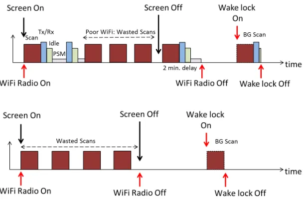
In a smart phone, a Wi-Fi scan is initiated in response to two actions: by turning on the screen or when an application specifically requests for a scan. When an AP is available to connect, the Wi-Fi driver scans the available channels and connects to the pre-configured AP as shown in Figure 4.1 (a). If no such AP is found in the pre-configured list, it periodically scans until the device is successfully connected to an AP or until a connection time-out occurs in the Wi-Fi driver after 15 mins.
Figure 4.1: Working of default Wi-Fi when (a) an AP is available to connect with, and (b) an AP is not available.
of 2 mins to avoid race conditions in the driver. CPU Wake locks are obtained for operations during screen off. While in connected state, if the link quality deteriorates, the Wi-Fi radio driver is kept in high power state constantly due to repeated scan and association requests. Also to avoid packet loss, the driver operates at lower modulation rates. Our measurements using a power monitor show the repeated scan/association operations in Figure 4.2.
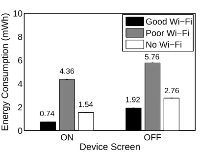
When there is no AP available to connect, the Wi-Fi radio driver scans continuously and results in energy wastage (Figure 4.1 (b)). The energy consumed by the Wi-Fi radio under various screen conditions and AP availability conditions is shown in Figure 4.3. Thus, PRiSM can save substantial energy by intelligently avoiding poor and no Wi-Fi conditions in an accurate manner.
4.2.2 Cellular Signatures
0 50 100 150 0 1000 2000 Time(sec) Power (mW) Screen ON Active Scan Association Fail Re−scan and Association Signal quality poor Re−association (a)
0 50 100 150
0 1000 2000 Time(sec) Power (mW) Active Scan Screen OFF
Background Scan to check new channel conditions Repeated High Power
Associations
(b)
Figure 4.2: Repeated scan/association events under poor AP signal when the device screen is (a) ON, (b) OFF.
ON OFF 0 2 4 6 8 10 Device Screen
Energy Consumption (mWh)
Good Wi−Fi Poor Wi−Fi No Wi−Fi 0.74 4.36 1.54 1.92 5.76 2.76
by the phones. A smart phone can receive signals from more than ten base stations (BSs) in dense urban areas [74]. GSM based Android phones can overhear signals from up to seven (six neighbouring and one connected) BSs in ASU (Active Set Updates) units at any time instant. The linear equation between dBm and ASU values for GSM networks isdBm= 2ASU −113. ASU values range from 0 to 31 and 99, which indicates unknown signal strength. The total time interval of observation of every base station within the signature differs and depends both on the total time spent by the user while connected to the particular Wi-Fi and also on the occurrence pattern of the base station.
To capture the entire signal characteristics that a user uniquely experiences for an AP, we propose to build cellular signal signatures using ‘‘probability distributions’’ of signal strengths from all observable connected and neighbor base stations rather than using abstracted information (e.g., ‘‘average signal strengths’’). A Wi-Fi signature is defined as the set of probability density functions (PDFs) of signal strengths from all connected and neighbor Base Stations (BS) when the smart phone is associated with that unique Wi-Fi AP. We performed the statistical measurements for all users in our dataset, but for explanation purposes, we will take random users to show the following results. Figure 5.4 shows the evolution of signatures recorded by a user over time for three Wi-Fi APs to which the user has connected most frequently. For better readability, we plotted only the signal strength distribution from the most frequently connected BS per Wi-Fi AP. The figure shows the PDF of signal strengths received from the connected BS at different intervals of time. Simply put, the distribution shown after 10 hrs includes the data used for the distribution shown at 5 hrs plus five more hours. Note that the signal strength distributions do not converge to a Gaussian distribution even after 25 hrs of signal accumulation. Hence, we develop a non-parametric algorithm which does not assume anything about the underlying data distribution. The correlation coefficient (ρX1,X2) between
0 5 10 15 20 25 30 0 0.1 0.2 0.3 0.4 0.5 P(X=x)
x: signal strength
14263 (13.128) 14261 (15.1878) 25763 (16.1716) 25762 (16.1678)
(a)
0 5 10 15 20 25 30
0 0.1 0.2 0.3 0.4 0.5 P(X=x)
x: signal strength
24262 (16.058) 24263 (16.1109) 24261 (6.66) 27162 (5.5312)
(b)
0 5 10 15 20 25 30
0 0.1 0.2 0.3 0.4 0.5 P(X=x)
x: signal strength
24262 (19.5635) 24263 (18.8606) 27162 (11.3358) 661 (12.7791)
(c)
Figure 4.5: The personalized signatures for three APs: (a) APX (b)APY, and (c)APZ. The
distance betweenAPX and APY is about 7km,APY and APZ is about 30meters. APY and
APZ are located in the same building. The observed base station IDs and their average signal
technique is likely to provide good performance in matching accuracy.
Figure 4.5 further shows that the signatures recorded by a user for different APs located far from or near to each other have significant dissimilarities. We again choose three Wi-Fi APs: APX,APY, andAPZ from a user’s database, where distances betweenAPX andAPY is about
7 km and betweenAPY and APZ is about 30 meters (APY andAPZ are in the same building).
In the figures, base station IDs and their average signal strengths are given in the legend. As expected, the signatures forAPX andAPY contain completely different sets of BSs and different
patterns of signal distributions. On the other hand, the signatures for APY and APZ show
similar sets of BSs. However, they are still distinguishable because the signal distributions show unique patterns. Considering the possible differences in the environment and the behaviour of a user, observing dissimilar signal distributions even for nearby APs is not surprising and actually helps to identify the APs more reliably.
4.2.3 Existing Localization Algorithms
A class of algorithms (referred as BSSET) uses the set of cellular BS ID’s to evaluate the likelihood of matching a fingerprint in the database. It can simply count the number of common BSs or can sum up the weight values of common BSs, where the weight is assigned to each BS based on its frequency of observation. Another set of algorithms (referred as MSE) use mean squared error for matching [59], [60]. An error is defined as the difference between the signal strength in current observation and the average signal strength recorded in the fingerprint for the same BS.
and hence, uses a specialized hybrid algorithm which includes lazy learning techniques and statistical likelihood estimation. Both BSSET and MSE algorithms need their own hard-coded threshold value (C) but PRiSM auto-tunes its threshold parameters regularly. Some others [33] use a model-based approach to build radio signal maps. They take more time to converge and require extensive war-driving to generate the data set. PRiSM does not assume anything about the underlying data model or distribution and hence takes a non-parametric approach.
4.2.4 Proposed Algorithm
We design an algorithm, ATiS, that can utilize detailed statistical properties of cellular signals instead of the averaged signal strength values. A simplified version of ATiS (Automatically Tuned Location Sensing) is explained in Algorithm 2. Since the entire signal distribution is available, ATiS predicts the location in near real-time. A higher level intuition of the algorithm is that if the probability of seeing a particular signal strength within the PDF of a base station (BS) is high and the probability of the BS observed when connected to an AP is high, the total
joint distribution is maximized and we get a more accurate signature match.
ATiS utilizes a set of signatures (P) each consisting of a set of base stations Rj and
corresponding signal strength distributions fk,j(S), where k∈Rj andj∈P. Note that j andk
are signature ID’s (e.g., Wi-Fi AP) and cellular base station ID’s respectively. Each signatureP has information pertaining to the number of occurrences made by its individual base stations in n(k, j) and the total occurrences of all its base stations collectively inNj. At any time interval
t ∈ [t1, t2] during the testing phase, the signal observed from a particular base station k is
measured to besk(t). For any signaturej which has observed this particular unique base station
over the course of its training time period, the likelihood of occurrence of the currently observed signals from the base station kis calculated as v(k, j) = (Qt2
i=t1fk,j(S =si(k))). Similarly, the
likelihood is calculated for every base stationk1,k2, ..knwhich is observed during the time frame
Algorithm 1: ATiS Signature Score Generation
1: INPUT:Signature database for all Wi-Fi APs connected by the user
2: INPUT:Set of currently observed BSs and their corresponding signal strengths at timet
3: INPUT:Hashmap of unique Wi-Fi APs and reverse Hashmap of observed BS IDs to APs for fast
lookup
4: OUTPUT:List of Wi-Fi APs in descending order of likelihood
5: Step 1.For given input BS, look-up the reverse Hashmap to identify the signature cluster subset to
reduce computation
6: Step 2.Calculate the score for the individual signatures
7: forall signatures in cluster subsetdo
8: forall Base Station ID0s within signaturedo 9: if Base Station ID exists in input at time(t)then 10: if Requested signal strength bin is Empty then 11: Normalize ‘x’ adjacent bins
12: end if
13: Evaluate likelihood of occurrence using expectation maximization from Bayesian-based ap-proach
14: end if
15: end for
16: Accumulate f inal likelihood scores f or all signatures
17: end for
18: Step 3.Apply the lower and upper bound thresholds ([CL, CU]) on generated scores
19: Step 4.Return Wi-Fi APs which satisfy the thresholds
20: Step 5.Check with the ground truth and update the signature thresholds if needed
j is then calculated ass(j) =
Q
k∈P(j)v(k, j)
.
Figure 4.6: PRiSM system architecture.
stations within a signature, the better is the score for the Wi-Fi. All signatures whose likelihood scores s(j) satisfy the lower bound (CL) and upper bound (CU) thresholds are returned as
output in descending order of their scores. Note that the values of [CL, CU] are initialized with
[1,0] initially and are decreased or increased over time to achieve a tight threshold range. The novel part of ATiS is that it auto-tunes thresholds within 0−1 based on likelihood scores by checking the ground-truth (i.e. Wi-Fi AP (un)available) after each connection attempt and hence, does not overfit the data for any particular scenario. Also, by design, PRiSM utilizes a
cluster-reduction approach to only compare the currently received signals with a small subset of the signatures in the database irrespective of the total database size and saves on computation time to compare from all the signatures otherwise.
4.3
Implementation
4.3.1 Architecture
Bootstrapping (signature collection
for each event)
Signature database
Cellular signal
observation Signature matching LBS Applications Query Relevant signatures Decision Online training (signal collection) Updated signatures Signatures Trigger
Figure 4.7: PRiSM operation includes three tasks: bootstrapping, signature matching, and online training.
decision engine ranks the scores from the Bayesian network based algorithm and outputs the result. The controller implements a novel selective-channel Wi-Fi scanning framework to connect to APs directly without scanning or association via wpa supplicant module in the phone system. It uses appropriate frequency channel information of APs stored in the database. The existing configuration file wpa supplicant.conf is intelligently modified at runtime to provide access to the manager and the controller simultaneously. Hence, PRiSM can serve as a middleware for all Location Based Service (LBS) applications in the smart phone. PRiSM suppresses Wi-Fi connection to an AP in poor signal strength regions and when the user moves closer to the same AP, it automatically matches the good signature of the AP and connects to it.
4.3.2 Operation
though not a main part of PRiSM operation, is shown here (shaded in Figure 4.7) since PRiSM also can serve as a middleware for all such applications in the smart phone. Only upon successful connection to an AP, we enterOnline Training through which the signature database is kept up-to-date. It is done to capture environmental changes such as configuration updates in an AP, changes in indoor signal propagation paths and behavioural changes in the user. PRiSM suppresses Wi-Fi connection to an AP in poor signal strength regions and when the user moves closer to the same AP, it automatically matches the good signature of the AP and connects to it.
When PRiSM predicts an AP, it tries to connect to the AP even without scanning. If the ground truth (checked by connecting to the AP after every prediction) has an AP (i.e., true positive), the connection attempt becomes successful and hence reduces the time to connect to an AP by 33.7%. If the ground truth has no AP (i.e.,false positive), the connection attempt will be unsuccessful and it auto-tunes the threshold parameters. PRiSM predicts no AP under two conditions: Zero Match (i.e., overheard BS ID’s do not match with any stored Wi-Fi signature) andThreshold Mismatch (i.e., overheard BS ID’s matched with some Wi-Fi signature but failed to satisfy the threshold parameters). In the case of zero match, PRiSM assumes the user is in a new place and scans all channels once to provide the results to the user. Here, it simultaneously aids for user experience and reduces energy on repeated scans until the user decides to connect to any AP. In the case of threshold mismatch, it first scans only those channels associated with its known list of APs in the database. If the scan results match with an AP in the database (i.e.,
4.3.3 Cost Analysis
Cellular signals are received and processed all the time by the phone MODEM at no extra cost. PRiSM activates the CPU only to read cellular signal values from the MODEM and to compute using ATiS. At all other times, CPU is not activated by PRiSM and consumes negligible energy (0.6 −1.1µW h) on top of CPU base energy. The sampling policy is shown in Table 4.1. The overall energy costs for continuous Wi-Fi sensing using PRiSM is minimal when compared to normal Wi-Fi scan. Using the reverse hashmap, the signatures are computed only for the MACs with current observed BS IDs. Hence, PRiSM only compares the currently received signals with a small subset of signatures in the database irrespective of the total database size and saves on computation time. Thus the space and time complexity needed for computation is a function of the density of APs in the nearby environment and is almost constant. In our traces, the signature comparisons never exceeded 35 even though some users had up to 337 unique signatures stored in their database. Hence, PRiSM is more robust to handle database explosion.
4.4
Evaluation
In this section, we will provide information about the datasets used in the experiments and the results obtained. The simulation and practical verification results are separately discussed.
Table 4.1: PRiSM cellular signal sampling policy.
Screen Wi-Fi State
Disconnected Connected
Table 4.2: Dataset information.
Dataset # of Volunteers Total hours Avg. Wi-Fi %
D1 24 2592 89.6
D2 16 1440 81.3
4.4.1 Datasets
We obtained Institutional Review Board (IRB) approval from North Carolina State University to gather datasets (Table 4.2) from Android based devices running our customized monitoring application. Data was collected for over two weeks from graduate students (29), undergraduate students (6), and employees (5). Undergraduate students predominantly covered locations within the campus. Graduate students had both on-campus and off-campus locations. Each employee data is from a different urban city in the US. The Android application using which the data was collected in shown in Figure 4.8. Since, the users were paid according to the number of hours they logged, the logging service also informs the number of hours the user has logged since the start. This is shown in Figure 4.9.
patterns and the number of unique locations visited throughout the data collection period.
(a) (b)
Figure 4.8: (a) shows the launch screen of the service where user information is gathered, (b) shows that the system service runs constantly in the background and logs all required
information.
4.4.2 Accuracy Measurements
(a)
Figure 4.9: The number of hours logged by each individual user is shown during data collection phase.
0 0.2 0.4 0.6 0.8 1 0 0.2 0.4 0.6 0.8 1 FPR(%) TPR(%) BSSET MSE ATiS (a)
0 0.2 0.4 0.6 0.8 1 0 0.2 0.4 0.6 0.8 1 FNR(%) TNR(%) BSSET MSE ATiS (b)
0 25 50 75 100 0 0.5 1 1.5 2 2.5
ρFN(%)
ρ FP (%) BSSET MSE ATiS (c)
Figure 4.10: (a, b) ROC curves and (c) ρF P Vs.ρF N values for a randomly selected user for
we observed a similar pattern across all users in the dataset.
False positive rate (FPR) is defined as the ratio of number of false positives over the sum of false positives and true negatives. True positive rate (TPR) is defined as the ratio of true positives over the sum of true positives and false negatives. Similarly True negative rate (TNR) is defined as the ratio of number of true negatives over the sum of true negatives and false positives. False negative rate (FNR) is defined as the ratio of number of false negatives over the sum of false negatives and true positives.
False positive ratio (ρF P) is defined as the number of cases that an algorithm detects an AP
when there is no such AP in the ground truth divided by the total number of cases. Similarly, false negative ratio (ρF N) is defined as the number of cases that an algorithm detects no AP
when there is an AP in the ground truth divided by the total number of cases. Higher ρF P
indicates losing more chances for energy saving and higherρF N indicates losing more connection
opportunities. Figure 4.10 (c) shows that BSSET and MSE class of algorithms require very high
1 2 3 4 5 6 7 8 9 10 0 0.5 1 1.5 2 2.5 Users Percentage (%) ρ FP ρFN (a)
1 2 3 4 5 0 0.5 1 1.5 2 Days Percentage (%) ρFP ρFN (b)
Figure 4.11: (a) AverageρF P andρF N for users in dataset ‘D1’ and (b)ρF P andρF N for 5
consecutive days for a user.
threshold values to achieve lower ρF P values, which results in undesired higher ρF N values.