University of Windsor University of Windsor
Scholarship at UWindsor
Scholarship at UWindsor
Electronic Theses and Dissertations Theses, Dissertations, and Major Papers
10-19-2015
Heuristics for Multi-Population Cultural Algorithm
Heuristics for Multi-Population Cultural Algorithm
Xinyu He
University of Windsor
Follow this and additional works at: https://scholar.uwindsor.ca/etd
Recommended Citation Recommended Citation
He, Xinyu, "Heuristics for Multi-Population Cultural Algorithm" (2015). Electronic Theses and Dissertations. 5639.
https://scholar.uwindsor.ca/etd/5639
This online database contains the full-text of PhD dissertations and Masters’ theses of University of Windsor students from 1954 forward. These documents are made available for personal study and research purposes only, in accordance with the Canadian Copyright Act and the Creative Commons license—CC BY-NC-ND (Attribution, Non-Commercial, No Derivative Works). Under this license, works must always be attributed to the copyright holder (original author), cannot be used for any commercial purposes, and may not be altered. Any other use would require the permission of the copyright holder. Students may inquire about withdrawing their dissertation and/or thesis from this database. For additional inquiries, please contact the repository administrator via email
Heuristics for Multi-Population Cultural Algorithm
by
Xinyu He
A Thesis
Submitted to the Faculty of Graduate Studies
through the School of Computer Science
in Partial Fulfillment of the Requirements for
the Degree of Master of Science at the
University of Windsor
Windsor, Ontario, Canada
2015
c
Heuristics for Multi-Population Cultural Algorithm
by
Xinyu He
APPROVED BY:
K. Tepe, External Reader
Department of Electrical and Computer Engineering
D. Wu, Internal Reader
School of Computer Science
Z. Kobti, Advisor
School of Computer Science
Authors Declaration of Originality
I hereby certify that I am the sole author of this thesis and that no part of this
thesis has been published or submitted for publication.
I certify that, to the best of my knowledge, my thesis does not infringe upon
anyones copyright nor violate any proprietary rights and that any ideas, techniques,
quotations, or any other material from the work of other people included in my
thesis, published or otherwise, are fully acknowledged in accordance with the standard
referencing practices. Furthermore, to the extent that I have included copyrighted
material that surpasses the bounds of fair dealing within the meaning of the Canada
Copyright Act, I certify that I have obtained a written permission from the copyright
owner(s) to include such material(s) in my thesis and have included copies of such
copyright clearances to my appendix.
I declare that this is a true copy of my thesis, including any final revisions, as
approved by my thesis committee and the Graduate Studies office, and that this thesis
ABSTRACT
Cultural Algorithm (CA) is one of the Evolutionary Algorithms (EAs) which
de-rives from the cultural evolution process in nature. As an extended version of the CA,
the Multi-population Cultural Algorithm (MPCA) has multiple population spaces.
Since the evolutionary information can be exchanged among the sub-populations, the
MPCA can obtain better results than the CA in optimization problems.
In this thesis, we introduce heuristics to improve the MPCA. The heuristic
strate-gies target the existing weaknesses in MPCAs. Four stratestrate-gies are developed
address-ing these weaknesses, includaddress-ing the individual memory heuristic, the social interaction
heuristic, the dynamic knowledge migration interval heuristic and the population
dis-persion based knowledge migration interval heuristic.Five standard benchmark
opti-mization functions with different characteristics are taken to test the efficiency of the
heuristics. Simulation results show that each heuristic, to varying degrees, improves
the MPCA in convergence speed, stability and precision. We compared different
combinations of the strategies, and the results show that the MPCAs with social
interaction based knowledge selection, as well as dynamic knowledge migration
inter-val/population dispersion based knowledge migration interval, outperform the other
DEDICATION
ACKNOWLEDGEMENTS
I would like to express my gratitude to all those who helped me during my graduate
studies. My deepest gratitude goes first and foremost to my supervisor, Dr. Ziad
Kobti for his constant support and guidance all throughout my graduate studies.
He has walked me through all the stages of the writing of this thesis. Without his
consistent and illuminating instruction, this thesis could not have reached its present
form.
My heartfelt gratitude goes to Mrs. Gloria Mensah, secretary to the director,
who has always helped setup meetings with my supervisor. In addition, my sincere
thanks to Ms. Karen Bourdeau, who has always been there to take care of other
issues related to my masters degree.
I am also indebted to NSERC Discovery Grants Program for partially supporting
my research.
Finally I would like to thank my parents for their unconditional support and love.
TABLE OF CONTENTS
AUTHOR’S DECLARATION OF ORIGINALITY iii
ABSTRACT iv
DEDICATION v
ACKNOWLEDGEMENTS vi
LIST OF TABLES x
LIST OF FIGURES xi
1 INTRODUCTION 1
1.1 Overview . . . 1
1.2 Motivation . . . 3
1.3 Problem Statement . . . 4
1.4 Organization of Thesis . . . 5
2 LITERATURE REVIEW 6 2.1 Evolutionary Algorithm . . . 6
2.1.1 Genetic Algorithm . . . 6
2.1.2 Particle Swarm Optimization . . . 8
2.1.3 Ant-colony Optimization . . . 9
2.1.4 Other EAs . . . 11
2.2 Cultural Algorithm . . . 13
3 PROPOSED ALGORITHM 19
3.1 Algorihtm Flowchart . . . 19
3.2 Knowledge Sources . . . 23
3.2.1 Normative Knowledge . . . 23
3.2.2 Topographic Knowledge . . . 26
3.2.3 Historic Knowledge . . . 29
3.3 Heuristic Strategies . . . 31
3.3.1 Strategy One (S1): Knowledge Selection Based on Individual Memory . . . 31
3.3.2 Strategy Two (S2): Knowledge Selection Based on Social In-teraction . . . 34
3.3.3 Strategy Three (S3): Dynamic Knowledge Migration Interval . 36 3.3.4 Strategy Four (S4): Population Dispersion Based Knowledge Migration Interval . . . 38
4 EXPERIMENT AND RESULT ANALYSIS 40 4.1 Benchmark Optimization Functions . . . 40
4.2 Experimental Setup . . . 45
4.3 Experimental Results and Analysis . . . 49
4.3.1 M1 vs. M2 vs. M3 . . . 49
4.3.2 M1 vs. M4 vs. M5 . . . 54
4.3.3 M1 vs. M6 vs. M7 vs. M8 vs. M9 . . . 55
4.4 Discussion . . . 59
4.5 A Real-World Application . . . 66
5 CONCLUSIONS AND FUTURE WORK 68
LIST OF TABLES
4.1 Dimensions, search ranges,and global optimum values of the test
func-tions . . . 40
4.2 Target values of 5 test problems [1] . . . 47
4.3 Main parameters for M1 vs. M2 vs. M3 . . . 49
4.4 Test result for M1 vs. M2 vs. M3 . . . 50
4.5 Main parameters for M1 vs. M4 vs. M5 . . . 54
4.7 Main parameters for M1 vs. M6 vs. M7 vs. M8 vs. M9 . . . 55
4.6 Test result for M1 vs. M4 vs. M5 . . . 56
4.8 Test result for M1 vs. M6 vs. M7 vs. M8 vs. M9(10-dimension) . . . 57
4.9 Test result for M1 vs. M6 vs. M7 vs. M8 vs. M9 (50-dimension) . . . 58
4.10 Test result for spring design problem . . . 67
LIST OF FIGURES
1.1 What is culture[2] . . . 2
2.1 Ants find the shortest path to the food[3] . . . 10
2.2 CA framework[4] . . . 13
2.3 MPCA framework . . . 16
3.1 Flowchart of the proposed MPCA . . . 20
3.2 Solution individual . . . 21
3.3 Cooperate mechanism of normative knowledge (m = 2) . . . 26
3.4 Topographic knowledge(2-dimension) . . . 27
3.5 Cooperate mechanism of topographic knowledge (m = 2) . . . 29
3.6 The memory can affect the individual’s decisions . . . 33
3.7 Individuals select knowledge source based on social influence . . . 35
3.8 Dynamic knowledge migration interval (ηmax = 50, N = 1.02) . . . . 37
4.1 3-D image for 2-D Sphere Function[5]. . . 41
4.2 3-D image for 2-D Schwefel Problem 1.2 Function[5]. . . 42
4.3 3-D image for 2-D Ackleys Function[5]. . . 43
4.4 3-D image for 2-D Rastrigin Function[5]. . . 44
4.5 3-D image for 2-D Rosenbrock Function[5]. . . 45
4.6 Ring topology, mesh topology and square topology . . . 48
4.7 Number of times three different knowledge sources being selected by individuals for F1 . . . 51
4.8 Number of times three different knowledge sources being selected by individuals for F2 . . . 52
4.9 Number of times three different knowledge sources being selected by individuals for F3 . . . 52
4.11 Number of times three different knowledge sources being selected by
individuals for F5 . . . 53
4.12 Convergence performance of M1,M3 and M9 for F1(10-D) . . . 60
4.13 Convergence performance of M1(constant knowledge migration inter-val = 1), M1(constant knowledge migration interinter-val = 6) and M8 for F2(50-D) . . . 61
4.14 Convergence performance of M1,M7 and M9 for F3 (50-D) . . . 62
4.15 Convergence performance of M1,M2 and M3 for F4(10-D) . . . 64
4.16 Convergence performance of M1, M8 and M9 for F5(10-D) . . . 65
1
INTRODUCTION
1.1
Overview
Optimization problems are crucial in Computer Science. Mathematical approaches
often meet failures in solving large-scale optimization problems. In addition to the
mathematical optimization, linear programming techniques and dynamic
program-ming techniques were developed to search for optimal solutions. However, these
techniques encounter difficulties again in solving the optimization problems with a
large number of variables as well as the optimization problems of non-linear objective
functions[7]. To overcome these problems, EAs were proposed by researchers. EAs
are a class of intelligent optimization algorithms that mimic the metaphor of gene
evolution and/or social behaviour of species[3], such as the behaviour of birds foraging
and behaviour of ants finding the route to the food source. However, EAs can only
get near optimal solutions. CAs are one of the most recent evolutionary algorithms
addressing these problems.
The term “culture” was first introduced by Edward B. Tylor in 1881. In his
bookPrimitive Culture, he described culture as “that complex whole which includes
knowledge, belief, art, morals, customs, and any other capabilities and habits acquired
Fig. 1.1: What is culture[2]
Inspired by the cultural evolution process in nature, an evolutionary
computa-tional system that can store, accumulate and utilize individuals’ experiences during
the evolution was proposed by Reynolds in 1994[4]. A CA system is divided into two
parts: population space and belief space. The two components evolve respectively and
communicate with each other by the communication protocol. The dual inheritance
structure makes the CA a self-adaptation system that enables global evolutionary
information be more fully utilized.
The MPCA is an extended version of the basic CA. In the standard CAs, the
in-fluence function guides the evolution only by the knowledge from a single belief space,
which may invalidate the structure of the CA and lead to poor global optimization
and instability. Therefore, the MPCA, a CA system with multiple populations was
proposed. The MPCA increases the validity of the knowledge by cooperating the
im-plicit knowledge from different populations and at the same time provides the optimal
1.2
Motivation
The CA has been proved a promising EA that can be widely used in many fields such
as complex global optimization problems, mechanical design[9], data mining[10][11]
and semantic networks[12], etc. As an extension of the CA, the MPCA has better
per-formance in avoiding premature convergence and convergence speed[13], so more and
more attention is directed toward the development of MPCAs. At present, MPCAs
still have some weaknesses that remain to be improved.
• The first weakness is that only the best solution coming from each sub-population
is able to be exchanged with the other sub-populations in terms of the given
communication rules. The best solution reflects not enough evolutionary
infor-mation, thereby decreasing the validity of cooperated knowledge. This probably
misleads the whole population converging to the local optima.
• The second one is the random knowledge selection strategy. When the MPCA
comes to the phase when the individuals select knowledge sources to evolve the
population, each individual selects the same knowledge source, and selects it in
a random way. The different categories of knowledge sources always have the
diverse influence on the individuals. For example, as the knowledge source used
to narrow the feasible search space, the normative knowledge source usually can
have more effect on the most individuals in the early stage of the evolution. The
topographic knowledge source can affect individuals more in the late time, as it
can direct the individuals to explore the search space more precisely. Therefore,
a more rational knowledge selection strategy for the individuals in the MPCA
need to be developed to improve the efficiency of the MPCA.
• The third weakness is that current MPCAs use the constant knowledge
migra-tion interval. Migramigra-tion and blend of knowledge sources among sub-populamigra-tions
at a too small interval may cause the loss of diversity for the population in the
early phase of the evolution. Therefore, current MPCAs require a more
rea-sonable strategy of knowledge migration interval that can manage knowledge
sources to be migrated at dynamic interval for different time of the evolution.
This weakness is also mentioned in the literature[13].
1.3
Problem Statement
Guo et al[13] developed a novel MPCA framework named Multi-Population Cultural
Algorithm Adopting Knowledge Migration (MPCA-KM). MPCA-KM provides the
approaches to overcoming the first drawback mentioned in Section 1.2. In this thesis,
we supplement the coordination mechanism of the normative knowledge source for
MPCA-KM and add a historic knowledge source to the algorithm. Then we apply
the proposed heuristic strategies to MPCA-KM. Benchmark optimization functions
with various properties are used to evaluate how these heuristics can improve the
algorithm’s efficiency in precision of solutions, stability and convergence speed. The
heuristic strategies are described as follows:
• The individuals in the population select the knowledge sources based on social
interaction.
• The individuals in the population choose the knowledge sources to based on
individual memory.
• The implicit knowledge sources migrate between sub-populations at the
dy-namic interval.
• The implicit knowledge sources migrate between sub-populations at the interval
Our target is to develop an enhanced MPCA by solving the existing weaknesses
mentioned in section 1.2. We anticipate these heuristics to improve the MPCA in
term of convergence speed, stability and precision.
1.4
Organization of Thesis
Chapter 2 contains a review of some typical EAs including Ant Colony Optimization,
Genetic Algorithms, and Particle Swarm Optimization. A review of previous works on
CAs and MPCAs is presented in Chapter 2. Chapter 3 details the descriptions of the
four heuristic strategies developed in this thesis. Chapter 4 produces the test results
and analysis of the four strategies and their combinations. Finally the conclusions
2
LITERATURE REVIEW
2.1
Evolutionary Algorithm
EAs are computational approaches that apply the natural biological evolution and/or
social behaviour of species to the problems of finding an optimal solution. In EAs,
the best solution is yielded from a population of candidate solutions. Part or all of
the population individuals (candidate solutions) would have to go through mutation,
crossover, selection and reproduction in each iteration of EAs. The operation of
muta-tion or crossover periodically makes changes in individuals of the current populamuta-tion,
producing the new individuals. The selection process makes the “most fit”
individ-uals survive, and eliminates the “least fit” members. Consequently, the surviving
individuals will participate in the next iteration. As a result of these steps, better
solutions will be produced along the iterations. However, EAs rarely reach the
opti-mal solutions because a solution can only be “better ” in comparison to the presently
known solutions. Some well-known EAs are Genetic Algorithm(GA), Particle Swarm
Optimization(PSO) and Ant Colony Optimization(ACO).
2.1.1 Genetic Algorithm
GAs originate from the idea of biological natural selection[14]. In GAs, solutions to
an optimization problem are represented as “chromosomes ”. A chromosome is made
up of a set of “genes” that express variables of the optimization problem. GAs start
with a random population of chromosomes. For each iteration of the GA, all the
chromosomes should be evaluated via the fitness functions. The chromosomes with
the best fitness value are selected to operate mutation and crossover so as to yield
the offspring chromosomes, and the offspring chromosomes will be taken to compare
with the parent chromosomes. Then, for steady versions of GAs, only the winning
for unsteady GAs, all the offspring solutions are used to form the population of next
generation without being compared with the parent solutions[3]. Usually, the process
of GAs is continued until a near-optimal solution is obtained, or a certain number of
generations is reached.
The main parameters used in GAs are population size, the maximum number of
generations, mutation rate, and crossover rate. Large population size and a large
num-ber of maximum generations usually gain the probability to obtain a better solution[3].
A small mutation rate is usually used, and the crossover is given a rate that ranges
from 0.6 to 1.0, traditionally[15].
A pseudocode for GAs is shown as follows[15].
Algorithm 1Genetic Algorithm[3]
1: Generate random population of P solutions (chromosomes); 2: for each individual i∈P do
3: Calculate f itness(i);
4: for each i= 1 to number of generations; do
5: Randomly select an operation(crossover or mutation);
6: if (crossover) then
7: Select two parents at random ia and ib;
8: Generate an of f spring ic=crossover (ia and ib);
9: else
10: if (mutation) then
11: Select one chromosome i at random;
12: Generate an of f spring ic=mutate (i);
13: end if 14: end if
15: Calculate the f itness of the of f spring ic;
16: if ic is better than the worst chromosome thenthen
17: replace the worst chromosome by ic;
18: end if 19: end for 20: end for
2.1.2 Particle Swarm Optimization
PSO was first proposed by Kennedy and Eberhart[16]. It is inspired by the social
behavior of a flock of birds that try to reach an unknown destination. A bird in the
flock is referred to a “particle” that is analogous to a chromosome in GAs. Particles
are unable to reproduce offsprings. Instead of reproduction, the particles change their
positions to evolve the populations. The particles have both private knowledge and
global knowledge which will help the particles approach the desired position (optimal
solution). In PSO, the particles can learn from their own experiment (local knowledge)
and can communicate with the other particles around them (global knowledge)[3].
The pseudocode for PSO is given as follows[17]:
Algorithm 2Particle Swarm Optimization[17]
1: Generate random population of N solutions(particles) 2: for each individual i∈N do
3: Calculate f itness(i);
4: Initialize the value of the weight factor, w; 5: for each particle do
6: Set pBest as the best position of particle i;
7: if fitness (i) is better than pBest; then 8: pBest(i)=fitness(i);
9: end if 10: end for
11: Set gBest as the best fitness of all particles;
12: for each each particle; do
13: Calculate particle velocity according to Equation 4; 14: Update particle position according to Equation 3;
15: end for
16: Update the value of the weight factor, w; 17: end for
18: Check if termination=true;
A PSO system is initialized with a swarm of random particles in a S-demension
space (S is the number of variables to the optimization problem). Each particle i is
assigned with three values: its current position (Xi), its velocity (Vi) and the best
current cycle (Pg) is also known to each particle in the population. Then for each
cycle, each particle updates its position according to the following formulas[18]:
N ew Vi =w×current Vi+c1×rand()×(Pi−Xi) +c2×Rand()×(Pg−Xi) (1)
N ew position Xi =current position Xi +new Vi ;
Vmax ≤Vi ≤ −Vmax
(2)
Here, w denotes the inertia weight that can balance the global search and local
search[18]. c1 and c2 are two positive constants called learning factors ,rand() and
Rand() generate a random number in the rang[0,1]. Vmaxis the upper bound to change
of velocity[16]. Four main parameters for PSO are the population size (number of
particles), number of generation intervals, the maximum change of the flying velocity
Vmax and the inertia weight w.
2.1.3 Ant-colony Optimization
ACO was developed by Dorigo et al.[19]. It takes inspiration from the natural fact
that ants are able to find the shortest path between their nest and the food source.
It is because ants leave a chemical substance named pheromone wherever they travel,
and ants follow the paths with more pheromone deposits. As shown in Figure 2.1,
the initial ants just randomly rotate around the obstacle on their first trip between
the nest and the food source. So the right direction and the left direction have the
same pheromone deposits. The ants travel the shorter path will find the food and
return earlier (assume all the ants have the same speed). Then the returning ants will
pheromone. Moreover, the ants that later start out will choose the shorter trial and
deposit more and more pheromone on the path. As a result of this positive feedback,
all the ants will finally choose the shortest path over time[20].
The pseudo code (Algorithm 2.1) from [3] describes how the basic ACO works and
there are many variations to this basic version[21].
Algorithm 3Ant Colony Optimization[3]
1: Initialize the pheromone trails and parameters;
2: Generate population of m solutions (ants);
3: for each individualantk i∈m do 4: Calculate f itness(k);
5: Determine its best position;
6: Determine the best global ant; 7: Update the pheromone trail;
8: end for
9: Check if termination = true;
Fig. 2.1: Ants find the shortest path to the food[3]
Similar to PSO, an ACO system starts with m random ants, and each ant carries a
solution string, withni optional values for each variable i. The selected value for each
variable represents the path which the ants will travel. The pheromone associated
with each path (optional value) will change iteratively as the following equations
τij(t) = ρτij(t−1) + ∆τij; t= 1,2..., T
∆τij = m X
R/f itnessk if option lij is chosen by ant k
0 otherwise
(3)
Here, τij(t) denotes the pheromone assigned with the ant i’s jth variable at the
tth iteration; ρ is the pheromone evaporation rate (0-1)[22]; ∆τij expresses the
in-creased pheromone deposits; R represents a constant number named pheromone
re-ward factor[3] that is used in minimization problems and lij denotes the jth option
for variable i. Then in the next iteration, the ant k will have probability Pij(k, t) to
choose the path lij according to the pheromone associated with the path.
Pij(k, t) =
[τij(t)]α×[ηij]β
P
lij[τij(t)]
α×[η ij]β]
(4)
As Formula 4 shown, ηij denotes the heuristic factor that can indicate how good
for ant k to choose option lij, α and β are two positive numbers that control the
importance of pheromone. The main parameters used in ACO are: the number of
ants, the number of iteration, pheromone evaporation rateρ, pheromone reward factor
R, α and β.
2.1.4 Other EAs
Other EAs including Evolutionary Programming (EP), Memetic Algorithm (MA) and
Shuffled Frog Leaping Algorithm (SFL) are briefly introduced as follows:
• Evolutionary Programming: The EP is a global optimization algorithm that
is similar to the GA. However, it only uses the Gaussian-based mutation
opera-tor to generate new candidate solutions. EPs are usually applied in continuous
• Memetic Algorithm: The MA was developed based on the notion of meme[24].
As the extension to the GA, the MA also has the chromosomes. However, the
elements that constitute the chromosomes are called memes. MAs use local
search technique, such as pair-wise interchange heuristics[25], to decrease the
likehood of premature convergence.
• Shuffled Frog Leaping Algorithm: The SFL algorithm is a multi-population
EA. In SFL algorithms, frogs(solutions) are divided into several sub-groups.
Within each sub-group, the frogs can exchange ideas with each other through
memetic evolution[26]. In addition to local search performing within each
sub-group, the evolutionary information is also passed among sub-groups in a
shuf-fling process.[27]
Many other EAs were developed besides the ones mentioned above. In general, we
do not have an EA that can optimize all the optimization problems, various EAs have
unequal performance for specific domains(see also the discussion on the no-free-lunch
2.2
Cultural Algorithm
Inspired by the process of social and cultural changes, the CA was developed to
enhance evolutionary computation. Besides the population component that
evolu-tionary computation approaches have, there is an additional peer component
be-lief space and a supporting communication protocol between these two components,
which makes CAs perform better in some special optimal cases than other EAs. The
following figure presents the basic CA framework[4].
Fig. 2.2: CA framework[4]
As Figure 2.2 shown, the population space and the belief space can evolve
re-spectively. The population space consists of the autonomous solution agents and the
belief space is considered as a global knowledge repository. The evolutionary
knowl-edge that stored in belief space can affect the agents in population space through
to belief space by the acceptance function. The population space in CAs can be
modeled by the population-based EAs, such as GAs[29], EPs[13] and PSO[30], etc.
In the process of the CA evolution, the population space is initialized with
can-didate solution agents at random, meanwhile, the initial knowledge sources in the
belief space are built. At first, the two spaces evolve independently. Then the
se-lected agents from the population space are used to update the belief space. After the
knowledge sources being updated, the belief space will reversely guide the evolution
of the population space. these procedures repeat till a termination condition has been
reached. The CA pseudo code presented by [10] is given as follows:
Algorithm 4Cultural Algorithm[10] 1: t=0;
2: Initialize Population POP(t); 3: Initialize Belief Space BLF(t);
4: Repeat
5: Evaluate Population POP(t); 6: Adjust (BLF(t), Accept(POP(t)));
7: Adjust (BLF (t));
8: Variation(POP (t) from POP (t-1)); 9: Until termination condition achieved
Different types of knowledge sources are used in the CA to solve different problems.
The researchers have concluded five categories of knowledge sources and all available
evolutionary information can be expressed by one of these five knowledge sources for
a given domain. They are:
• Situational Knowledge: Chung[31] proposed the situational knowledge in
1997. It is designed to solve real-valued function optimization problems in the
static environment. The situational knowledge can record the exemplars of
successful and unsuccessful solutions.
• Normative Knowledge: The normative knowledge describes ranges of
can induce individuals to evolve within the domain that has the larger likehood
to obtain optimal solutions.
• Topographic Knowledge: The topographic knowledge sources can express
the spatial pattern of individual’s behavior. The topographic knowledge is
usually used to exploit the search space more precisely by dividing the space
into smaller cells[32].
• Domain Knowledge: To solve dynamic optimization problems, Reynolds and
Saleem introduced the domain knowledge to CAs[33]. It is used to monitor the
changes of the environment and predict the evolutionary trend.
• Historic Knowledge: The historic knowledge was also proposed by Reynolds
and Saleem[33]. The historic knowledge can be considered as the log in which
2.3
Multi-Population Cultural Algorithm
Researchers have developed many CAs with single population space. These CAs
are powerful and perform well on a wide variety of problems. However, it has been
proven that the CA system with multiple population spaces can reach better solutions
to the optimization problems[34]. The MPCA enables implicit knowledge sources
to be exchanged among sub-populations based on certain rules. With knowledge
sources from different sub-populations migrated and cooperated with each other, the
individuals can obtain more evolutionary information to evolve the population more
quickly and more precisely. Consequently, the MPCA can improve the speed of
convergence and have more probability to overcome premature convergence. The
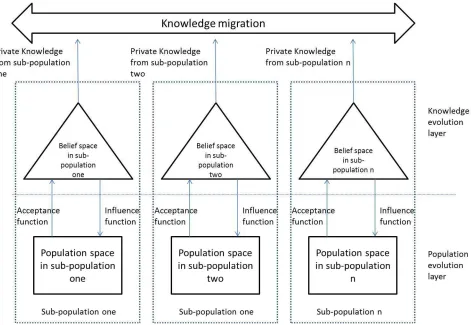
following diagram describes an MPCA framework proposed by Guo et al[13].
As the Figure 2.3 shown, an MPCA system contains n sub-populations. Each
sub-populations is a basic CA system that consists of belief spaces and population
spaces. Each sub-population evolves independently for a certain generations, and then
the knowledge sources in the sup-populations will be migrated to each other. The
migrated knowledge source from the other sub-population will blend with the private
knowledge sources, as so to form the new private knowledge sources. By the way
of knowledge migration, the evolutionary information extracted from different
sub-populations will be shared with all the individuals. It is noted that, the knowledge
migrations happen at a certain generation interval. The details of the migration
strategies of different knowledge sources are discussed in Chapter 3.
The brief review of some current MPCAs is presented as follows:
• Digalakis and Margaritis[34] proposed an MPCA called the parallel co-operating
cultural algorithm (PARCA). The PARCA consists of several sub-components
and each of the them runs a CA with different hehaviour. Local search is
adopted by each sub-component. They claimed that the exchange of
informa-tion among the sub-CA systems allows them to co-operate and explore
promis-ing areas of the search space found by the other populations, and also to
rein-troduce previously lost cultural material in the population. However, the
sub-populations in PARCA exchange the information extracted only from the best
solution individual. This may reduce the accuracy and stability of the
algo-rithm.
• Alami et al.[35] proposed an MPCA using fuzzy clustering. The proposed
MPCA uses the fuzzy clustering technique to divide the initial population into
sub-populations, and each sub-population can be managed by their own local
CA. Besides, it introduces the cultural exchange concept that can be useful
to mining new cultural. They declared that the experimental results indicated
fitness technique on four known multi-modal test functions. However, their
model cannot support multiple types of knowledge sources for being migrated
among sub-populations.
• MPCA-KM is a novel MPCA framework that was developed by Guo et al[13].
Guo et al. declared that MPCA-KM has faster convergence speed and better
solutions than CA and PARCA for the high-dimensional static optimization
problems. In MPCA-KM, the information is shared among sub-populations in
the forms of different knowledge types. They introduce the knowledge
coopera-tion strategy of topographic knowledge, but more cooperacoopera-tion strategies need to
be developed for the other categories of knowledge sources. Moreover, the model
does not consider the knowledge selection strategies when the MPCA-KM uses
more than one knowledge source. They illustrated that the MPCA-KM requires
a dynamic knowledge migration interval among sub-populations for the future
work.
We have reviewed many EAs in this section. In summary, a GA has a simple
structure that cannot store the individuals’ knowledge over long time; For PSO, the
individuals can communicate with each other, but only in one form where the
individ-uals gather toward to the best solution; ACO is mainly used for discrete optimization
problems that are not the domain that our work focuses on; CA can store and utilize
various forms of knowledge, but the social contact is restricted to a single
commu-nity. MPCA models have not only individual-to-individual social interaction, but
community-to-community social interaction as well, that is more fit to natural
sys-tem than single-population CA models. Therefore, our heuristics are built on the
3
PROPOSED ALGORITHM
In this chapter, we introduce the flowcharts of the proposed MPCA and the
pro-posed MPCA will be compared with MPCA-KM. We subsequently discuss the design
of knowledge sources that used in the proposed MPCA and how these knowledge
sources migrate among the sub-populations. Last, the four heuristics that apply to
the proposed MPCA are presented.
3.1
Algorihtm Flowchart
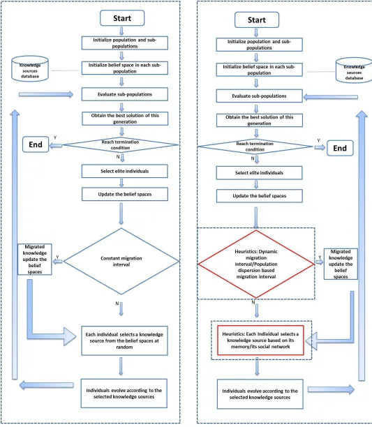
Figure 3.1 shows the flowcharts of both the MPCA-KM and the proposed MPCA. The
parts wraped by the dotted line are the components to which the heuristic strategies
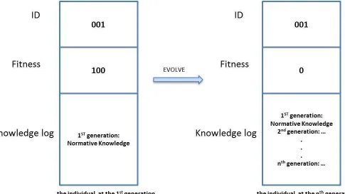
To observe the influence of the proposed heuristic strategies, each solution
(indi-vidual) in the proposed MPCA is assigned with a unique ID that will not be changed
during the whole process of the evolution as well as a knowledge-log that can record
which and how the knowledge source impact the evolution of the individual in each
generation. Figure 3.2 shows the sample of an individual in the proposed MPCA.
Fig. 3.2: Solution individual
Algorithm 5MPCA with the proposed heuristics 1: Parameters initialize;
2: Generate random population of n solutions (individuals);
3: Initial population is divided into M sub-population denoted by Pi, i=1,2,...,M;
4: for each belief space∈ Pi do 5: Initialize knowledge sources;
6: end for
7: for each individual x∈ Pi, i=1,2,...,M do 8: calculate fitness(x);
9: end for
10: for each Pi do
11: Sort the individuals according to fitness value;
12: Select p% top individuals;
13: for each private knowledge source do
14: Update according to Formula (6)(7)(8)(9)(12)(17) in Section 3.2;
15: end for 16: end for
[Heuristics about knowledge migration interval ]
17: g←dynamic interval heuristics or population dispersion based interval heuristics [Heuristics about knowledge migration interval ends ]
18: if generation = g then
19: for each sub-population having adjacent sub-populations do
20: knowledge sources to be migrated to the adjacent sub-populations←private knowledge sources;
21: new private knowledge sources ←blend(private knowledge, migrated knowl-edge from the adjacent sub-populations) according to Formula (11)(15); 22: end for
23: end if
[Heuristics about knowledge selection ] 24: for each individual x∈ Pi, i=1,2,...,M do
25: Select one knowledge source from the belief space; [ Heuristics about knowledge selection ends ]
26: x¯ ← evolve(x, the selected knowledge source) according to Formula (10)(14)(18);
27: if fitness(¯x) is better than fitness(x) then 28: x¯ replaces x;
29: end if 30: end for
3.2
Knowledge Sources
The CA enables the evolutionary information to be collected, stored and updated in
the belief space as knowledge source. Along with the development of CAs, it was
concluded that five knowledge sources are are able to express all available knowledge
for a given domain[36]. Each of these five knowledge sources is suitable to specific
optimization problems. In our thesis, normative knowledge, topographic knowledge,
and historic knowledge are used for the proposed MPCA, as the heuristic strategies
primarily focus on the static environment. The update of the knowledge sources is
discussed in this section, which refers to the 14th step in Algorithm 5. The evolution
of individuals that controlled by the three knowledge sources refers to the 26th step
in Algorithm 5 and the process of knowledge sources blend is related to the 21ststep
of Algorithm 5.
3.2.1 Normative Knowledge
Normative knowledge is used to define the feasible search space to an optimization
problem. According to [31], the normative knowledge of the ith sub-populationPi is
described as follows:
N Ki =< Iji, Lij, Uji > (5)
Here, j = 1,2, ...m, m denotes the number of variable of the optimization problem.
Ii
j = [lij, uij] records the bound of feasible search space to the jth variable, andlji and
ui
j express lower bound and upper bound, respectively. For instance, I11 = [−10,10] means that lower limit and upper limit of the first variable in the first sub-population
are -10 and 10. Lij expresses the fitness score of the lower bound of the jth variable.
Similarly, Uji denotes the fitness value of the upper bound of the jth variable.
elite individuals as follows[31]:
lij(t+ 1) =
xilj(t) if xilj(t)< lij(t) or f(xil(t))< Lij(t)
lji(t) else
(6)
Lij(t+ 1) =
f(xilj(t)) if xilj(t)< lii(t) or f(xil(t))< Lii(t)
lij(t) else
(7)
uij(t+ 1) =
xilj(t) if xilj(t)> uij(t) or f(xil(t))< Uji(t)
uij(t) else
(8)
Uji(t+ 1) =
f(xilj(t)) if xilj(t)> uji(t) or f(xil(t))< Uji(t)
Uji(t) else
(9)
Here, formula(6) and (7) represent the update for lower bound for thejthvariable
and its lower fitness value at the (t+1)th generation. Then equation(8) and (9)
represent the update for upper bound of the jth variable and update of the upper
bound’s fitness value. Within these formulas, xilj(t) denotes value of the jth variable
of the lthindividual in the ithsub-population, andf(xil(t)) indicates the fitness score
of individual, xi l(t).
Suppose xi
lj(t) select normative knowledge at the tth iteration; it is induced to
evolve by the normative knowledge source in the following way[31]:
¯ xilj(t) =
xikj(t) + δ 2(u
i j(t)−l
i
j(t)) if x i
lj(t)∈I i j
δ(uij(t)−lji(t)) +lij(t) if xilj(t)∈/ Iji
(10)
Here, ¯xilj(t) is the value of the jth variable to the individual xilj(t) after evolving,
and δ is a random number between 0 and 1. As the formulas shown, normative
knowledge utilizes the information that is carried by the elite individuals to reduce
space, thereby avoiding inefficient search outside the dominant landscape.
In our proposed MPCA, each sub-population evolves independently. Therefore,
the belief spaces of different sub-populations have varying degree of development. To
increase the efficiency of the algorithm, sub-populations need to share their private
knowledge with each other. Thereby the knowledge sources of more developed
populations need to cooperate with the knowledge sources of less developed
sub-populations.
Suppose the normative knowledge source N Km in the belief space of the mth
sub-population migrates to the belief space of the ith sub-population and cooperates
with the normative knowledge source N Ki. This will cause the N Ki to be updated
as follows:
N Ki =
N Km if ∀j ∈[1, m], Iji ∈Ijm and Lmj ≤Lij and Ujm ≤Uji
N Ki else
(11)
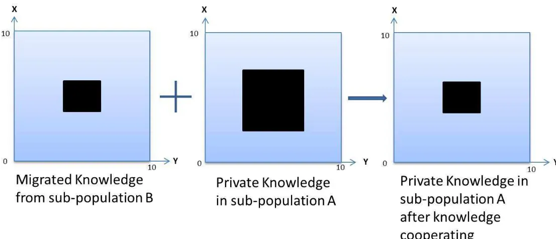
Figure 3.3 shows an example of normative knowledge sources that come from two
populations blend. The black boxes represent the feasible search space in
sub-population A and sub-sub-population B. Obviously, the sub-sub-population B has a more
developed normative knowledge source, which has narrowed the feasible space to
a smaller region. After blending with the normative knowledge source from
sub-population B, the normative source in sub-sub-population A will evolve to the same range
as the normative knowledge source in sub-population B. The migration of normative
knowledge can speed up the evolution of the belief spaces in sub-populations so as to
Fig. 3.3: Cooperate mechanism of normative knowledge (m = 2)
At the early stage of evolution, normative knowledge can guide the population
explore the whole search space and quickly identify the dominant regions. However,
after the individuals gather at the regions with the most potential, normative
knowl-edge is unable to drive them into exploiting the regions more precisely.
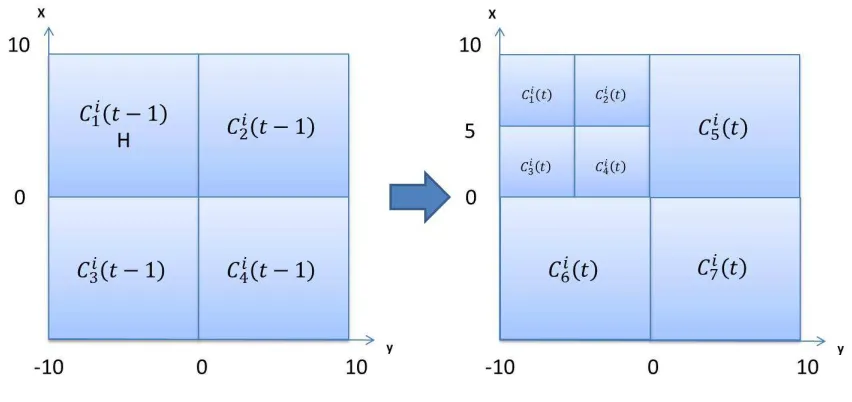
3.2.2 Topographic Knowledge
Topographic knowledge describes the distribution of good solutions in the feasible
search space. Within the search space recorded by normative knowledge, the area
containing the best solution is uniformly divided into subspaces along each dimension
by a binary tree. Thereby, the m-dimension hypercubes with the same size are formed.
The hypercubes are called cells. Obviously, there are 2m cells. Assume the best
solution at the t−1 iteration is located in a 2-dimension area [(-10,10),(-10,10)], and
four cells are obtained in this area, noted by C1i(t−1), ..., C4i (Figure 3.4). Then, if
four cells again, as shown in Figure 3.4.
Fig. 3.4: Topographic knowledge(2-dimension)
Topographic knowledge composed of cells is described as follows[32]:
T Ki(t) =< C1i(t), C2i(t), ...Cki(t), ... > (12)
Each cell is assigned an attribute about the potential to get the optimal solution.
Cell attribute =
High(H) f(xik∗)>f¯(xik∗)
U nknown(#) xi(t)∈/ Cki(t)
Low(L) f(xik∗)≤f¯(xik∗)
(13)
In formula 13, f(xi∗
k) denotes the fitness value of the best individual in the kth
cell and then ¯f(xik∗) expresses the average performance value of the best individuals
from all cells. The cell attribute shows the possibility of a cell containing the global
optimal solution. H means the cell is a possible subspace finding the better solutions.
# means a cell has not been explored. In order to determine whether good solutions
Topographic knowledge is used to induce individuals to exploit certain cells,
namely local search. Topographic knowledge evolves the individuals in the
follow-ing way[32]:
¯ xilj(t) =
xikj(t) +δ f(x
i l(t))
Pn
l=1f(xil(t))
(uij(t)−lij(t)) if (xilj(t)∈/ Cki(t))∩(attributeik 6=L)
xilj(t) + δ m
q f(xi
lj(t)) if (x i
lj(t)∈C i
k(t))∩(attribute i k =H)
(14)
As above mentioned, cells with H or # attribute shall be mainly searched. If the
individuals are located in the cells with H, they will search for the optimal solutions
amongst these cells. If the individuals are located in cells with L attribute, they will
move towards the cells with better potential.
Topographic knowledge directly influences the exploitable ability of the individuals
to the dominant region. Different sub-populations may have topographic knowledge
sources of different development. A reasonable strategy of cooperating topographic
knowledge sources from different sub-populations is important. [13] provides a
cooper-ate mechanism to topographic knowledge. Suppose T Kj =< Cj
1(t), C
j
2(tC
j
3(t), C
j
4(t), C5j(t), C6j(tC7j(t), >is the topographic knowledge in the jth sub-population at the tth
generation as shown in Figure 3.5, andT Ki =< Ci
1(t), C2i(tC3i(t), C4i(t), C5i(t), C6i(tC7i(t) >is the topographic knowledge from the ith sub-population as shown in Figure 3.5.
Then, if the knowledge migration condition is satisfied at the the tth generation,T Kj
and T Ki will mix to form the new topographic knowledge T Kij(t).
Fig. 3.5: Cooperate mechanism of topographic knowledge (m = 2)
3.2.3 Historic Knowledge
In this thesis, historic knowledge is designed to record the good solutions that have
been found, which can be represented as follows:
HKi(t) =< E1i, E2i, ...Eji, ....Esi > (16)
Here, s is maximum length ofHKi,Ei(t) = [xi
t] ,xit denotes the best individual of
theith sub-populationtiterations ago and t≤s. The historic knowledge database can
be described as a queue. Once the queue is full, the new coming record will replace
the most recent record which has been stored in the queue. The update of historic
knowledge is shown as follows:
HKi(t+ 1) =
< Ei(1), Ei(2), ...Ei(t), Ei(t+ 1)> if t < s
< Ei(1), Ei(2), ...Ei(s)> if t ≥s
(17)
To avoid missing potential region, historic knowledge induce individuals to search
sources work, Gaussian mutation[37] will be adopted in the vicinity of the best
solu-tions at the early stage of the evolution. The influence function relevant to historic
knowledge is given in Equation 18, Si denotes a random individual selected from
SKi, and w
1, w2 represent the weight parameters, w1, w2 ≥0 and w1+w2 = 1. δ is a random number between 0 and 1.
3.3
Heuristic Strategies
In order to improve the weakness in current MPCAs, which are the random
knowl-edge sources selection mechanism and the constant knowlknowl-edge migration interval, four
heuristic strategies applied to the different components of MPCAs are proposed. The
four heuristic strategies are knowledge selection based on individual memory,
knowl-edge section based on social interaction, dynamic knowlknowl-edge migration interval and
population dispersion based knowledge migration interval.
3.3.1 Strategy One (S1): Knowledge Selection Based on Individual
Mem-ory
Utilizing more than one type of knowledge sources enable MPCAs to solve more
complex optimization problems. However, different categories of knowledge sources
have different effectiveness for the entire population from early time to latter time
of the evolution. Furthermore, for an individual, the effectiveness of every type of
knowledge source will change along with the evolution, since the individual’s position
will change over the evolution. For example, an individual that has been very close to
the optimal solution can get more benefit from topographic knowledge sources than
normative knowledge sources, since the topographic knowledge sources can guide the
individual search for the space more precisely.
The individuals in existing MPCAs cannot identify the importance of knowledge
sources, thereby they choose random knowledge sources to evolve the population,
which may reduce the efficiency of MPCAs. Therefore, a novel knowledge selection
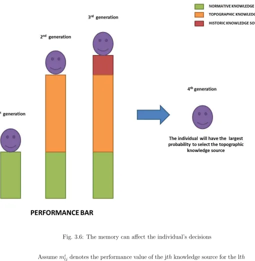
heuristic strategy is introduced in this thesis. It is assumed that the individuals have
memory of the knowledge source’s performance, due to which they are more likely to
select the knowledge source that has better performance. Figure 3.6 shows an example
of how an individual that has memory selects the better knowledge source. The
normative knowledge source, topographic knowledge source, and historic knowledge
source in order. The height of the bar represents the fitness value of the individual.
The topographic knowledge source gain the height fitness bar most. Therefore, the
individual is most likely to select the topographic knowledge at the fourth generation.
It is noted that:
• The individuals only have short-term memory. That is only the most recent
performance of each knowledge source can be kept for the individuals;
• The higher performance value one knowledge source has, in the larger possibility
the individual will select the type of knowledge source in the next round;
• The initial performance value of all knowledge sources are zero;
• If the performance value of all three types of knowledge sources for the individual
are zero, the individual will select each of the three types of knowledge sources
Fig. 3.6: The memory can affect the individual’s decisions
Assume mi
lj denotes the performance value of the jth knowledge source for the lth
individual in the ith sub-population. Then the update of mi
lj is shown as follows:
milj =|f itness(xil(t+ 1))−f itness(xil(t))|
if xil selects the jth knowledge source at the tth generation
(19)
next generation is defined as:
pilj = m
i lj
Pn
j=1m
i lj
(20)
where n denotes the total number of available knowledge sources.
Algorithm 6 describes the MPCA with knowledge selection based on individual
memory. Algorithm 6 refers to [Heuristics about knowledge selection ] in
Algorithm 5.
Algorithm 6MPCA with knowledge selection based on individual memory 1: for each individual x∈ Pi, i=1,2,...,M do
2: update(mi lj)
3: if ∀j ∈[1, n], milj = 0 then
4: xi
l will select normative knowledge source, topographic knowledge source,
and historic knowledge source in order in the next three generations; 5: else
6: xi
l selects the one knowledge source j according to probability pilj;
7: end if 8: end for
3.3.2 Strategy Two (S2): Knowledge Selection Based on Social
Interac-tion
Knowledge selection strategy based on social interaction is proposed for the same
purpose as knowledge selection strategy based on individual memory. It is assumed
that the individuals have social connections with each other in the population. The
individuals’ choices can be affected by their “neighbours” in the population[40]. For
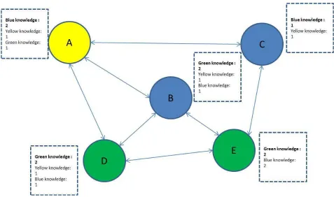
example, as the Figure 3.7 shown, it is a simple social network for a 5-individual
population. The circle with different colours represents the individual that want to
suggest the knowledge source of that color to its neighbours. Then, the individuals
will transit their knowledge suggestions to their neighbours(adjacent individuals).
For instance, individual A will transit the suggestion of selecting yellow knowledge
the network. Then every individual counts up the knowledge source suggestion bids
collected (include the original knowledge suggestion hold by the individual itself ).
The knowledge source type that has most votes will be selected by the each individual
in next iteration. In the example of figure 3.7, individual A has collected two blue
knowledge suggestions, one yellow knowledge bid and one green knowledge suggestion,
so A will select blue knowledge source.
Fig. 3.7: Individuals select knowledge source based on social influence
For this heuristic strategy, it is noted that:
• Which knowledge source the individuals suggests to its neighbors is determined
by the individual memory developed in strategy one;
• If there are ties between knowledge sources bids, the individual will select the
• There are different types of social network topology. The efficiency of different
social network used in the algorithm will be discussed in the next chapter;
• Each sub-population has independent social network;
Algorithm 7 shows the MPCA with knowledge selection based on social
inter-action. Algorithm 7 refers to [Heuristics about knowledge selection ]
in Algorithm 5.
Algorithm 7MPCA with knowledge selection based on social interaction 1: for each individual x∈ Pi, i=1,2,...,M do
2: update(milj) 3: if ∀j ∈[1, n], mi
lj = 0 then
4: xil will suggest normative knowledge source, topographic knowledge source, and historic knowledge source in order over next three generations;
5: else
6: xil suggests the knowledge source j according to pilj 7: end if
8: end for
9: for each Pi do
10: for each Individual do
11: Transmits the suggested knowledge source to the adjacent individuals.
12: Counts the bids of collected knowledge sources
13: if There are ties between knowledge sources then 14: Selects the suggested knowledge source
15: else
16: Selects the knowledge source that has most votes 17: end if
18: end for 19: end for
3.3.3 Strategy Three (S3): Dynamic Knowledge Migration Interval
As discussed in section 1.2, constant knowledge migration rate that apply to the
exist-ing MPCAs may result in premature convergence and more convergence generations
for optimization problems. At the latter time of evolution, the diversity to individuals
up the pace on convergence. On the other hand, the frequent migration of knowledge
at the early time decrease the diversity of individuals, this may lead the algorithm
trapping in the local optima.
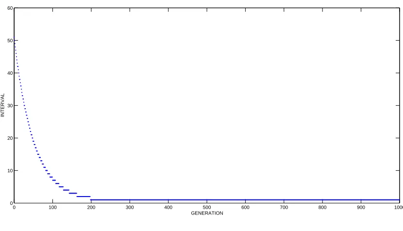
Therefore, a dynamic knowledge migration rate is introduced as followed[38]:
η(t) =f loor(ηmaxN−t+ 1) (21)
Here, η denotes the number of iteration between two knowledge migrations ,ηmax
denotes the maximum interval,η∈[1, ηmax] and N reflects the rate of interval change,
N >1.
Figure 3.8 shows an example of knowledge migration interval. The maximum
interval is 50 generations at the beginning of evolution; then the interval gradually
decreases to 1 at around the 200th generation.
0 100 200 300 400 500 600 700 800 900 1000
0 10 20 30 40 50 60
GENERATION
INTERVAL
Fig. 3.8: Dynamic knowledge migration interval (ηmax = 50, N = 1.02)
Algorithm 8 describes the MPCA with dynamic knowledge migration interval and
5.
Algorithm 8MPCA with dynamic knowledge migration interval 1: update(η);
2: g← η+generation of previous knowledge migration
3.3.4 Strategy Four (S4): Population Dispersion Based Knowledge
Mi-gration Interval
This strategy is put forward for the same purpose as strategy three. MPCAs need an
indicator to determine when to migrate the knowledge sources among sub-populations.
Therefore, we use population dispersion rate to decide the timing of knowledge
mi-gration. Population dispersion was proposed by Lisis [39]. It is used to measure the
intensity of the population.
P D(t) =
n X j=1 [ 1 popsize popsize X i=1
(xij(t)−
1 popsize
popsize
X
i=1
xij(t))2] (22)
In formula 22, P D(t) refers to the dispersion rate of the entire population at
the tth generation, xlj(t) represents the jth variable of the lth individual at the tth
generation.
It is assumed that:
• If P D(t) > τ, τ is a positive number. The distribution of individuals in the
population space is scattered, the knowledge sources of each sub-population do
not migrate at the tth iteration. This will maintain the high diversity of the
population.
• If P D(t) ≤ τ, the distribution of individuals in population space is
concen-trated, the private knowledge of each population will migrate to other
Algorithm 9 shows the MPCA with dynamic knowledge migration interval and
refers to [ Heuristics about knowledge migration interval] in Algorithm
5.
Algorithm 9MPCA with population dispersion based knowledge migration 1: update(P D(t));
2: if P D(t)> τ then
3: g ← 0;
4: else
4
EXPERIMENT AND RESULT ANALYSIS
In this chapter, we first introduce the test functions for the experiment. Then we
explain the detail of the experimental setup. Last, the summary results of the tests
along with the analysis will be presented.
4.1
Benchmark Optimization Functions
Many commonly used benchmark optimization functions are used to evaluate and
compare the performance of optimization algorithms. In our experiments, five static
minimal optimization functions[5] with different characteristics are taken to test the
proposed heuristic strategies. All of these test functions are dimension-wise scalable.
1. F1(x) = PD
i=1x 2
i
2. F2(x) = (PDi=1(Pij=1xj)2)
3. F3(x) = −20exp(−0.2 q
1
m
PD
i=1x 2
i)−exp[
1
m
PD
i=1cos(2πxi)] + 20 +e
4. F4(x) = PD
i=1(x 2
i −10cos(2πxi) + 10)
5. F5(x) =
PD−1
i=1 (100(x2i −xi+1)2+ (xi−1)2)
Table 4.1: Dimensions, search ranges,and global optimum values of the test functions
Function Dimension Search range Optimal solution Global
minima
F1:Sphere f unction 10/50 xi∈[−100,100] [0,0, ...,0] 0
F2:Schwef el problem 10/50 xi∈[−100,100] [0,0, ...,0] 0
F3:Ackley f unction 10/50 xi∈[−30,30] [0,0, ...,0] 0
F4:Rastrigin f unction 10/50 xi∈[−5.12,5.12] [0,0, ...,0] 0
F1 (Sphere Function) : As the figure 4.1 shown, sphere function is simplest
uni-modal function in the test functions. It is featured with uniuni-modal, separable
and dimension-wise scalable.
Fig. 4.1: 3-D image for 2-D Sphere Function[5].
F2 (Schwefel Problem 1.2 Function) : As shown in figure 4.2, the global minimal
solution is located in narrow and long area. Schwefel problem 1.2 function is
Fig. 4.2: 3-D image for 2-D Schwefel Problem 1.2 Function[5].
F3 (Ackley Function) : Ackley function is a multi-modal optimization function
which has a lot of local minima. A large number of modals(local minima) are
located in a very flat area(figure 4.3) due to modulation of added amplified
cosine wave. It is featured with multi-modal, non-separable, and
Fig. 4.3: 3-D image for 2-D Ackleys Function[5].
F4 (Rastrigin Function) : Rastrigin function has lots of local minimas in the range
[-5.12,5.12], seen from figure 4.4. It is featured with multi-modal, separable,
Fig. 4.4: 3-D image for 2-D Rastrigin Function[5].
F5 (Rosenbrock Function) : Rosenbrock function is a multi-modal optimization
function which the global minima is located in a very narrow and long bar-type
area. It is featured with multi-modal,non-separable,dimension-wise scalable,
Fig. 4.5: 3-D image for 2-D Rosenbrock Function[5].
These different types of benchmark optimization test functions with different
char-acteristics are appropriate for evaluating the performance of the proposed algorithm.
4.2
Experimental Setup
We perform the experiments to compare the performance between MPCA with the
proposed heuristics and MPCA without the heuristics (MPCA-KM) on the five test
functions. Furthermore, we compare the efficiency of different heuristic strategies.
The combinations of the strategies explained in Chapter 3 and their abbreviations
• M1: Basic MPCA without heuristics
• M2: MPCA with knowledge selection based on individual memory heuristics
• M3: MPCA with knowledge selection based on social interaction heuristics
• M4: MPCA with dynamic knowledge migration interval
• M5: MPCA with population dispersion based knowledge migration interval
• M6: MPCA with knowledge selection based on individual memory heuristics
and dynamic knowledge migration interval
• M7: MPCA with knowledge selection based on individual memory heuristics
and population dispersion based knowledge migration interval
• M8: MPCA with knowledge selection based on social interaction heuristics and
dynamic knowledge migration interval
• M9: MPCA with knowledge selection based on social interaction heuristics and
population dispersion based knowledge migration interval
The nine algorithms listed above fall into 3 sets: M1 vs M2 vs M3, M1 vs M4 vs
M5 and M1 vs M6 vs M7 vs M8 vs M9. For a fair comparison, the algorithms in the
same set use the same parameters given in Table 4.3, Table 4.5 and Table 4.7 . All
the experiments are carried out with JAVA language. For the purpose of reducing
statistic error, sixty trial runs are performed for each function. The performance of
the different algorithms was compared using the following criteria:
1. Mean fitness: mean value of the solutions got at the maximum generation in 60
runs.
3. Interval number: The average value of iteration number to reach the target
so-lution value in 60 runs. The target soso-lution value is usually within an acceptive
tolerance of the known global optima for an optimization function. The target
values to the five test functions are summarized in table 4.2.
Table 4.2: Target values of 5 test problems [1]
Function Target
F1(10-Dimension) 1× 10⁻⁸
F1(50-Dimension) 1× 100
F2(10-Dimension) 1× 10⁻¹
F2(50-Dimension) 1× 10³
F3(10-Dimension) 1× 10⁻¹²
F3(50-Dimension) 5× 100
F4(10-Dimension) 1× 101
F4(50-Dimension) 3× 10²
F5(10-Dimension) 1× 10⁻¹
F5(50-Dimension) 1× 10²
It is noted that the different topologies used in the social network model for
connection between individuals have the different effect on the efficiency of strategy
two. There are three commonly used topologies supported in population-based EAs
[40]. The efficiency of using the three topologies in Strategy two is discussed in the
next chapter. The three topology types are:
• Ring topology: Each individual has two connections to other individuals in the
population. (figure 4.6 b)
• Square topology: Each individual has four connections to other individuals in
• Square topology: Each individual has connections to all other individuals in the
population. (figure 4.6 a)
4.3
Experimental Results and Analysis
4.3.1 M1 vs. M2 vs. M3
Table 4.3: Main parameters for M1 vs. M2 vs. M3
Parameter Value
Population size 200
Sub-population amount 8
Sub-population amount size 25
Selection proportion 0.3
w1: weight parameter in Formula 18 0.7
w2: weight parameter in Formula 18 0.3
Constant knowledge migration interval 3
Run times 60
Maximum iterations 1000
Dimension 10
Table 4.4 show the test result of M1, M2, M3 using ring topology, M3 using square
topology and M3 using mesh topology on benchmark optimization functions F1-F5.
The best results got in 60 runs are typed in bold. It can be observed that the
pro-posed two heuristic strategies in term of knowledge selection improve the performance
of original MPCA in mean fitness value, standard deviation, and iteration number.
Furthermore, all three M3s outperform M2 on the five test functions. For the
compar-ison of the M3s adopting different topologies, M3(Square topology) can get the best
fitness value and the smallest standard deviation in 1000 generations, and M3(Mesh
topology) can use the minimal generations to reach the target fitness value on all the
five optimization problems. However, the difference of test results between the M3s
using different topologies is minor.
Figure 4.7 - Figure 4.11 show that over 1000 generations, how many times an
for F1 test function, by average, an individual select normative knowledge 563 times,
topographic knowledge 425 times and historic knowledge 12 times, in M3. Obviously,
without knowledge selection strategies, the individual select almost same amount of
three knowledge sources in original MPCA(M1). The two knowledge selection
heuris-tics can drive the individuals to select more normative knowledge and topographic
knowledge, and much less historic knowledge. This can improve performance of the
MPCA, as normative knowledge, and topographic knowledge can give the individual
much greater probability to find a better solution than historic knowledge. In the
other word, historic is the weak knowledge compared with normative knowledge and
topographic knowledge.
Fig. 4.7: Number of times three different knowledge sources being selected by
Fig. 4.8: Number of times three different knowledge sources being selected by
indi-viduals for F2
Fig. 4.9: Number of times three different knowledge sources being selected by
Fig. 4.10: Number of times three different knowledge sources being selected by
indi-viduals for F4
Fig. 4.11: Number of times three different knowledge sources being selected by
![Fig. 2.2: CA framework[4]](https://thumb-us.123doks.com/thumbv2/123dok_us/1396766.1172375/26.612.116.555.253.554/fig-ca-framework.webp)
![Fig. 4.1: 3-D image for 2-D Sphere Function[5].](https://thumb-us.123doks.com/thumbv2/123dok_us/1396766.1172375/54.612.134.521.156.473/fig-d-image-for-d-sphere-function.webp)