Error Compensation Using Inverse Actuator Dynamics

(1)

ABSTRACT

PANUSITTIKORN, WITOON Error Compensation Using Inverse Actuator Dynamics (Under the direction of Thomas A. Dow.)

The use of Non-Rotationally Symmetric (NRS) optical surfaces has increased significantly in recent years. These surfaces can be quickly machined using a diamond turning lathe and a Fast Tool Servo (FTS). However, the dynamic response of the actuator influences the output tool motion resulting in form errors. This dissertation describes an open-loop command modification technique, also know as a deconvolution operation, that can significantly reduce tool motion errors. The technique uses knowledge of the gain and phase response of the dynamic system and the information content of the driving command to modify the amplitude, phase and shape of the input command signal. The modified command signal creates the desired tool motion.

(2)

The tool trajectory of an FTS is dependent on the spindle speed and the cross-feed rate which may drift over a long fabrication time and an NRS feature can contain varying amplitude. To address these issues, two adaptive modification schemes using the Short-Time Fourier Transform (STFT) and an equivalent inverse dynamics filter were proposed. These schemes can account for the changing frequency and amplitude content of the driving command using the most recent machining conditions and the appropriate transfer function.

(3)

ERROR COMPENSATION USING INVERSE ACTUATOR DYNAMICS

by

WITOON PANUSITTIKORN

A dissertation submitted to the Graduate Faculty of North Carolina State University

In partial fulfillment of the Requirements for the Degree of

Doctor of Philosophy

MECHANICAL AND AEROSPACE ENGINEERING

Raleigh 2004

(4)

(5)

BIOGRAPHY

(6)

ACKNOWLEDGEMENT

I wish to express my most sincere gratitude and appreciation to my advisor. Prof. Thomas A. Dow, for his guidance, support and insights he has towards research, which made this dissertation possible. I admire the persistent attitudes and his sense of humors, which may be some of the most valuable lessons that I take with me from my tenure in NC State. He is one of the most accessible and open-minded advisors one can ever find.

My heartfelt gratitude goes to Ken Garrard for his side-by-side assistance and valuable advice in a lot of ways. I always respect him as another advisor of mine. Appreciation is also extended to Alex Sohn for his enthusiasm, technical assistance on the ASG 2500 DTM and instrumentation. Special thanks go to Chris Wildsmith and Matias Heinrich of Vistakon, who initiate this research.

I am grateful to Dr. Paul Ro, Dr. Jeffrey Eischen and Dr. Gregory Buckner, for serving on my Advisory Committee. Their time, patience and encouragement along the way is certainly appreciated. Thanks also go to Dr. Gail Jones and Dr. Zhilin Li, who acted as Grad School representatives.

(7)

I The fellowship I’ve received from the FRIDAY GANG is a rare gift one can possess. always consider myself as a lucky one who is surrounded by great people. Thanks for all prayers, encouragement and patience that allows me to be me.

(8)

LIST OF TABLE

(13)

LIST OF FIGURES

1-1 Diamond turning machine (orthogonal stages and air bearing spindle) and a fast tool servo ...3

1-2. The base machine generates a cylindrical surface while the FTS

superimposes a sine wave feature ...3

1-3. The FTS inscribed a 10µm P-V sine wave into a brass cylinder ...4

1-4. Geometric description of the ring gauge...4

1-5. The FTS axis trajectory composes a relatively higher frequency than the

base machine axes ...6

1-6. A spiral path overlaid the part represents a tool excursion associated with a

spindle speed and a cross feed ...7

1-7. An attenuated output excursion with a phase angle of an actuator due to its

dynamic characteristics ...9

1-8. Dynamics of the FTS influences form errors of the machined surface ...9

2-1. Spring-mass-damper system ...19

2-2. Dynamic response of a FTS can be presented in either the frequency or the

time domain ...20

(14)

2-4. An example of aliasing where a 21 Hz sine wave (solid line) is sampled at 21 Hz (dots) and the reconstructed signal (dashed line with dots) is a 1 Hz

sine wave...23

2-5. Superposition shows how the final output is generated...24

2-6. Impulse response is the outcome of a normalized impulse to a system...25

2-7. Input decomposition to different forms of the components...26

s s 2-8. The vector repeats itself at f =…, −F (or –20Hz),0, F (or 20Hz),… ...28

2-9. Discrete Fourier Transform of a normalized impulse...30

2-10. Frequency response of the desired excursion ...32

3-1. Variform fast tool servo ...34

3-2. Diagram of frequency response measurement ...35

3-3. Frequency response of the Variform at 20µm P-V amplitude...36

3-4. The complex number form of the frequency response at 20µm P-V...38

3-5. Impulse response of the Variform fast tool servo...38

3-6. Desired signal yd[n] and modified input signal xm[n] obtained by deconvolution...39

3-7. Path error associated with a modified input and unmodified input ...39

3-8. Modified and unmodified inputs at low amplitude (±4 volts) ...40

3-9. Path error due to modified and unmodified inputs at low amplitude (±80 µm)...40

(15)

3-11. Path error due to modified and unmodified inputs at high amplitude

(±200µm) ...41

3-12. The slope of the modified command signal response reaches the maximum value due to the physical limits...41

4-1 FTS response associated with a 200 Hz, 300µm P-V input signal and its velocity...43

4-2 Frequency analysis of the distorted output trajectory ...44

4-3 3D frequency response as a function of input amplitudes ...45

4-4 Operating range of the Variform...45

4-5 Phase of the tool motion measured by the LVDT and a capacitance gauge (inverted) with respect to a 100 Hz input signal ...46

4-6 Dynamic response measured by the LVDT with respect to the capacitance gauge ...46

4-7 Single-pass laser interferometer configuration ...48

4-8 Acquisition sequence of the Axiom 2/20 series...48

4-9 Acquisition the Axiom 2/20 series using the dSPACE...50

4-10 The measurment setup on an optical table ...51

4-11 A wrapped around profile of a swept sine wave...52

4-12 An unwrapped profile of the FTS motion with respect to the desired and the signal measured by the LVDT ...52

(16)

4-14 Dynamic characteristics of the Variform position sensor...54

4-15 Nonlinearity of the Variform to various amplitudes of input command signals ...55

4-16 Amplitude dependent modified input signals ...57

4-17 Influence of the nonlinearity to the path differences with respect to the desired trajectory...58

4-18 Comparison of the desired and the actual tool trajectory associated with the amplitude of the desired trajectory...59

5-1 Rectangular and triangular windows draw a short piece out of a long signal ...62

5-2 Overlap-add method reconstructs the original signal from small pieces ...63

5-3 Schematic of the short-time Fourier transform...64

5-4 Reconnection process of complete modified input signals...65

5-5 Simulation results of the STFT deconvolution ...67

5-6 Experimental results of the STFT deconvolution in real-time ...68

5-7 Frequency spectrum of the equivalent inverse dynamic filter ...69

5-8 Block convolution using the overlap-add method ...71

5-9 Modified input command signal reconstruction using the overlap-add method...72

5-10 Block convolution using the overlap-save method ...73

(17)

5-12 Comparison of a sinc function and a sine wave...76

5-13 The inverse Fourier transform of the frequency response ...77

5-14 Group delays of all FTS responses are less than 4 samples...78

5-15 Shifted impulse response of the FTS ...79

5-16 Shifted inverse dynamics filter ...79

6-1 Tool cutting motion along spiral path to create a concave sphere ...82

6-2 Create an amplitude map of the desired surface ...84

6-3 The tool radius compensation for an off-axis sphere...85

6-4 Comparison of the desired surface and the tool path due to tool radius compensation ...86

6-5 Generate a spiral pattern over the machined part...86

6-6 Acceleration reduction at sharp corners...87

6-7 On-axis sphere diamond turned on copper-plated blocks...88

6-8 Interferometer shows the form error of 12.6 nm RMS ...89

6-9 The roughness of the on-axis sphere is 3.5 nm RMS ...89

6-10 An input command signal and its frequency response of the off-axis sphere ...90

6-11 Comparison of the deconvolution and the gain and phase correction ...91

6-12 Path differences associated with modified and unmodified input signals ...92

(18)

6-14 Comparison of the profiles of the machined surfaces in the tool trajectory

direction ...93

6-15 With a lower spidle speed, the modification yielded even better form

fidelity ...94

6-16 The shape of the reflection at the center of the spherical features clearly

show the form error of the machined surfaces...95

6-17 Figure error when measuring the modified surface in cross feed direction...97

6-18 A cylinder cavity with a full cosine wave cross section ...98

6-19 The cosine profile of the test part has a frequency component close to the

peak of the gain response and near the physical limits of the Variform...99

6-20 A simulated output tool path associated with a modified input command

signal yielded the path difference of 200 nm P-V ...99

6-21 Comparison of the path differences associated with the modified and

unmodified input commands...100

6-22 The velocity profiles of the modified and unmodified tool path ...101

6-23 The machined surface associated with the modified and unmodified input

commands ...102

6-24 Direction of the profile measurement with respect to the reference flat...103

6-25 The surface profile measurements of the modified and unmodified

surfaces ...105

6-26 The cause of the form errors in the machined surface is the wrong spindle

(19)

A-1 Schematic of input command modification using the pole-zero

cancellation ...119

A-2 Comparison of desired and modified input command using pole-zero A-3 Phase response of the output excursion with respect to the desired tool A-5 Steady state path difference as applying the closed loop pole-zero cancellation ...119

path...120

A-4 Schematic of the pole-zero cancellation in a feedback loop...120

cancellation (model)...121

B-1 Diagram of a reference capacitor loop...123

B-2 Control diagram of the Variform FTS ...125

B-3 Force directions on the T-lever ...125

C-1 Schematic of an inverse amplifier...130

E-1 Tool center is shifted in x and w direction to compensate for the nose radius...133

G-1 Desired and modified input command signals...145

G-2 Difference of the modified input command signals...146

(20)

G-4 Modified input command signal using a block deconvolution and gain

scheduling scheme ...147

G-5 Velocity of the modified input signal exceeds the physical limits of the

Variform...148

G-6 Tool trajectories associated with transfer functions of 120 and 240 µm P-V...149

(21)

CHAPTER 1 INTRODUCTION

The use of high precision components with more advance, and more complex geometry has increased significantly in both military and civilian applications, particularly for optical systems [1]. A turning process with a diamond cutting tool can produce machined surfaces with high form fidelity and short production time in which traditional sequential processes of milling, grinding, and polishing hardly accomplish. In lights of the development of fluid-mechanic systems, laser interferometers, temperature and vibration controlled environments, and axes feedback controllers, the improved quality of diamond turned surfaces can be advantageous to all optics industry.

1.1 D

IAMOND

T

URNING AND

F

AST

T

OOL

S

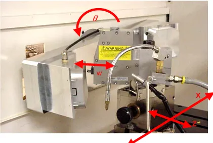
ERVO

(22)

the workpiece on a spindle causes a symmetric surface to be machined. Advantages of diamond turning are reduced process time as compared to fly-cutting due to the continuous high cutting speed achieved via rotation of the workpiece, excellent form fidelity and optical quality surface finish. It is desirable to produce optical systems with the diamond turning process that have high spatial frequency features or are non-rotationally symmetric (NRS). The addition of a high-bandwidth actuator is one technique [2-4] that has been used to add low amplitude, sub-revolution features to an asphere or sphere. Examples include torics and off-axis segments of a conic machined on center. Figure 1-1 illustrates a configuration of machining a NRS feature; a DTM is moving its orthogonal axes in x and z directions, and spinning an arm that holds a part off the rotational axis while a FTS is moving in and out in

w direction as a function of θ to generate a high spatial frequency component.

Another demonstration of machined part realized by rotation of a diamond turning machine (DTM) and sinusoidal motion of a fast tool servo (FTS) is a fabrication of inertial confinement fusion targets [13]. These parts were for an investigation of a physics phenomenon at Los Alamos National Labs. Sine wave feature with constant amplitude and frequency was produced on the OD of a brass cylinder as depicted in Figure 1-2.

Challenges of this fabrication were the small size of part, as shown in Figure 1-3, and the

(23)

X

Z

θ

w

Figure 1-1. Diamond turning machine (orthogonal stages and air bearing spindle) and

a fast tool servo

Figure 1-2. The base machine generates a cylindrical surface while the FTS superimposes a

(24)

Figure 1-3. The FTS inscribed a 10µm P-V sine wave into a brass cylinder

(a) A ring gauge measurement artifact (b) A sine wave feature with varying spatial frequencies inscribed on the ID of the gauge

(25)

Another demonstration of high precision fabrication is a metrology artifact (or a ring gauge) for a Coordinate Measuring Machine (CMM) [14]. An aluminum ring as shown in Figure 1-4(a) was inscribed with a varying-spatial-frequency sine wave on the ID to determine any anomalies on a surface that contribute to a measurement. The sine wave feature had fixed

amplitude of 5µm P-V and continuously increasing wavelength from 0.00125” to 0.250”

over the first quadrant of the ring. The other 3 quadrants had mirror images of the first quadrant as shown in Figure 1-4(b).

1.2 NRS F

ABRICATION

The examples of the last section illustrate a range of possible surface shapes feasible using a FTS on a diamond turning machine. Some use the FTS to create the surface on a cylindrical face (fusion targets and ring gauges.) Others require coordinated motion of the FTS and the axes as a function of x, w, and θ to produce the desired surface shape, such as the off-axis

conic machined on axis. In this case, the NRS component is superimposed on the best fit asphere.

(26)

1.2.1 Static Decomposition

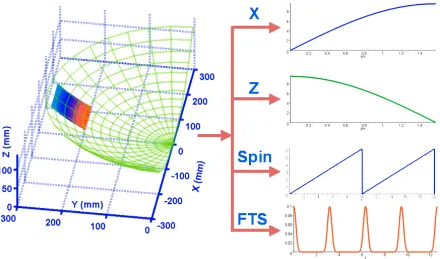
The motion commands for each axis of the base machine and the FTS must be generated from a 3D geometric description of the desired part. While the fusion targets and the ring gauges are on the cylindrical surface, the features must be located, in some cases, with respect to some reference angle on the part. The part shape must be decomposed into a rotationally symmetric (RS) surface of revolution (i.e., a cross section) for the diamond turning machine (DTM) and a spindle angle dependent motion path of a non-rotationally symmetric (NRS) surface for the FTS. In Figure 1-5, while the DTM axes move to machine an asphere (or RS surface), the FTS superimposes a high frequency feature (or NRS surface).

Figure 1-5. The FTS axis trajectory composes a relatively higher frequency than the base

(27)

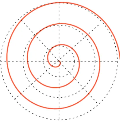
The knowledge of a desired trajectory is available in advance by decomposing a 3D geometric description and superimposing a spiral pattern to describe a trajectory of a tool center as shown in Figure 1-6.

Figure 1-6. A spiral path overlaid the part represents a tool excursion associated with a

spindle speed and a cross feed

The principle difficulty is that while the FTS has a high relative bandwidth, it has a limited range of motion when compared to the other axes of the DTM. This surface decomposition process has been solved for a variety of shapes and will not be addressed.

1.2.2 Dynamic Convolution

(28)

small lag time associated with an FTS will result in poor form fidelity for off-axis surfaces and improper placement of NRS features with respect to the rotationally symmetric (RS) base surface and any fiducial. The heterogeneous nature of the axes can result in phase errors in the recomposition of the decomposed command signals. The example in Figure 1-5 shows that the decomposed FTS motion changes direction at least once on each rotation of the spindle whereas the axis motions are almost always in one direction (a waxicon being a notable exception). The phase errors of the base machine axes can usually be ignored as the axis accelerations are moderate and velocity tracking performance of the control system is quite good. However, the FTS usually requires higher acceleration and velocity.

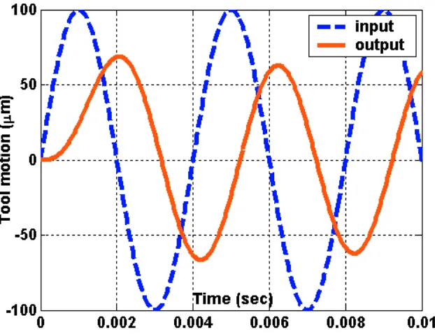
All linear systems including actuators exhibit gain and phase response to varying input command signals. In Figure 1-7, an output response (a solid line) associated with a 250 Hz sinusoidal input signal (a dash line) is a sine wave with its input frequency, but with attenuated amplitude and a phase delay.

(29)

Figure 1-7. An attenuated output excursion with a phase angle of an actuator due to its dynamic characteristics

(30)

A first order correction of the FTS phase error is to apply a constant lead time to its motion commands. The magnitude of this phase advance depends only on actuator bandwidth and spindle velocity. However, for motion paths that use a substantial portion of the bandwidth range or contain frequency components close to the bandwidth of the axes, this simple technique yields poor results. The response of a dynamic system to an applied signal is a function of the frequency of that signal. In general, the response results in an attenuated and out-of-phase motion of the output with respect to the input signal. When the system is a fast tool servo and the dynamic input signal is made up of a variety of frequencies, the result is form error in the machined surface.

1.3 R

EVIEW OF

L

ITERATURE

(31)

Implementation using stable poles and zeros approximates known resonance, attenuation modes and damping factors of the dynamic system to shape the closed-loop characteristics. As a result, it is sensitive to unknown dynamics, and the unity gain response is limited to the resonant frequencies of the unstable zeros.

Zero Phase Error Tracking Control (ZPETC) [6-10] is a digital feedforward and look-ahead control algorithm that modifies the pole-zero cancellation to reject the dynamic response of stable poles and well-damped zeros. Using knowledge of (entire or partially-known in advance) desired trajectories compensates phase responses of lightly damped.

Feedforward ZPETC has been used in many control schemes such as digital tracking control [6-7] because knowledge of the entire tool excursion is available. A series of feedforward corrective gains expressed by the unstable zeros of the system was attached to exponentially reduce the ZPETC tracking error [8]. A continuous-time control algorithm of the ZPETC [9] was developed with a series of gain compensation for a sinusoidal trajectory. An adaptive control cascading a digital prefilter (DPF) to the ZPETC [10] improves gain and phase response with a low computation cost.

(32)

resonate an input command signal at harmonic frequencies and eliminate the path error. This control scheme is limited to periodic input command signals.

Another breakthrough of an input command modification technique is an input shaping technique [13] that reduces residual vibration of a flexible mechanical system when following an instantaneous change direction trajectory such as a step. The scheme has been applied to many systems such as a computer disk drive, nanopositioners, etc. Though it seems to be a promising command modification scheme for many applications, the technique does not meet a fundamental requirement of a precision machining; the scheme does not correct errors due to the phase response.

(33)

1.4 O

BJECTIVES

O

F

T

HE

R

ESEARCH The objectives of the research are as follows:

1. To investigate the dynamic response of a tool axis to an input command signal and construct an algorithm to characterize the inverse of the FTS dynamics

2. To improves the form fidelity of non-rotationally symmetric (i.e., spindle angle dependent) surfaces machined on a diamond turning lathe by incorporating knowledge of the desired surface and the dynamics of a tool axis into the tool path generation process.

3. To discover the range and quality of features that can be fabricated using the tool axis and then to use that information to select the cutting conditions that optimize the desired surface.

1.5 O

UTLINE OF

D

ISSERTATION

(34)

Chapter 3 introduces a procedure of measuring the dynamic response of an actuator. Then, the FTS will make use of this measurement to perform a preliminary test on the deconvolution. Frequency components of a desired trajectory will be chosen close to the FTS bandwidth, which a output motion is nearly an inverse of its applied input signal. Summary of a significant improvement will, consequentially, be drawn from both simulation and experimental results.

The implementation issues that have came across in the test will be discussed in Chapter 4. Physical limitation plays an important role to describe an operating range of the modified algorithm. Another issue is a hidden dynamic response of an internal position sensor of the Variform FTS. Accordingly, the fault monitored tool motion clouded the true performance of the inverse dynamics algorithm. A use of an laser interferometer will be discussed in detail to identify the actual characteristic of the actuator.

The feedforward and look-ahead scheme can also use a small sliding window of trajectory data to improve tracking performance and to reduce the overshoot of an accelerated axis. Chapter 5 will discuss practical implementation methods of block convolution. Short-Time Fourier Transform and equivalent inverse dynamics filter break a long signal of a desired input command into short pieces before performing the inverse dynamics algorithm.

(35)

(36)

CHAPTER 2 CONVOLUTION AND DECONVOLUTION

This chapter describes the fundamental mathematics that relates the input command signal, the system dynamics, and the gain and phase response of the output motion. Based on specific assumptions to establish an operating range, the inverse of this input/output operation can be used to create a modified input command that will produce the desired output. Digital Signal Processing (DSP) and Discrete Fourier Transform (DFT) can be used to transfer time-based signal into the frequency domain. Note that the technique can be applicable to any dynamic system; however, for the application in this dissertation (diamond turning of non-rotational symmetric surfaces), the system are electro-mechanical linear and rotary axes. These include a fast tool servo, a long range tool servo, and a rotary tool servo.

2.1 L

INEAR

, T

IME

-I

NVARIANT

S

YSTEM

(37)

characteristics between an output and input signal when the form of the output signal is a copy of the input, but with different phase and amplitude. And it also means that transfer function of the system does not change with time. Figure 1-7 is a good illustration of this property. To its input signal, the response conforms with the same frequency though it is out of phase and has smaller amplitude. Note that the command modification techniques discussed in Section 1.3 also require this assumption.

In addition to the homogeneity, another property of a linear system is the superposition principle; a signal can be decomposed into a number of sub-signals which when applied to the system produce the same result as their sum. These homogeneity and superposition yield an alternative way to determine an output signal by decomposing the input signal into sub-signals, applying the signals individually to the system resulting in sub-output sub-signals, and finally recomposing them to the output.

Mathematically, when a linear system is driven by a periodic function x(t) with an amplitude A and a frequency of ω radians per second, the steady-state output motion y(t) is attenuated by a gain factor a and is phase shifted by an angle φ.

Input: x(t) = Asin(ωt)

Output: y(t) =a Asin(ωt +φ)

(38)

frequency components each of which will be attenuated and delayed. The response of the system y(t) will be the sum of these frequency components.

Input: x(t) =

∑

A_isin(ω_it) i

Output: y(t) =

∑

ai Ai sin(ωi t +φi ) i

To machine a desired surface profile with high fidelity, the amplitude attenuation and phase related delay must be eliminated. To achieve this, the input signals are modified prior to applying them to the system such that the attenuation is canceled and the phase is compensated. After the dynamics of the system are identified and the desired motion is

decomposed into sinusoids, amplitude ( ai) and phase (φi) adjustments can be found to manually construct a modified command that moves the actuator in the desired manner.

Modified Input: x(t) =

∑

Ai

sin(ω_it −φ_i) i ai

Desired Output: y(t) =

∑

a_iAi

sin(ω_it +φ_i−φ_i) i ai

This manual method is slow and cumbersome if the signal contains many frequency components. However, the DSP and DFT can be used to minimize the effort. A technique for system identification and an input signal modification algorithm have been developed and applied to a tool axis to produce the desired output response for high frequency inputs.

(39)

Fast Tool Servo (FTS)) implements a reference capacitor loop control (discussed in detail in Appendix B) to linearize its closed-loop performance with a broad bandwidth. Despite achieving the linear characteristics, the FTS output shows gain and phase response of a second-order system and is equivalent to a response of a spring-mass-damper system as shown in Figure 2-1. An input command is influenced by the dynamics of the system resulting in an output excursion with an attenuation and a phase delay.

Figure 2-1. Spring-mass-damper system

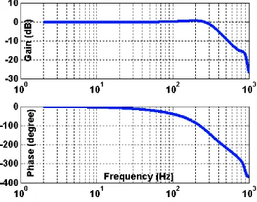
The dynamic response of an FTS can be presented in either the time domain (impulse response) or the frequency domain (frequency response). They are both shown in Figure 2-2 and are mathematically equivalent and complete for a linear system. On the left in Figure 2-2(a), the top graph shows the ratio of the amplitude of the output to the input (in dB1 units) as a function of frequency. At low frequency, the output is equal to the input and the ratio is unity giving a dB value of zero. As the frequency is increased, the amplitude response peaks

dB=20 log10

⎛ ⎜⎜ ⎝

output⎞

⎟⎟ ⎠

input

(40)

at about 200 Hz and then drops rapidly for higher frequencies. The lower graph in Figure 2-2(a) shows the phase angle between the input and the output. At lower frequencies these signals are nominally in phase, but even a small lag of less than a degree represents a significant length of arc if the actuator is used at a large radius from the axis of spindle rotation. As the frequency rises, the output increasingly lags the input. At 100 Hz this lag is about 45º and at 340 Hz it is about 180º.

The impulse response is shown on in Figure 2-2(b) and describes the response of the system with respect to time for an impulse at time zero. The Fourier transform of the impulse response is exactly equal to the frequency response and the inverse Fourier transform of the frequency response is the impulse response.

(a) Dynamic response of a Variform FTS (b) expressed in the time domain expressed in the frequency domain

Figure 2-2. Dynamic response of a FTS can be presented in either the frequency or the time

(41)

2.2 D

IGITAL

S

IGNAL

P

ROCESSING

(DSP)

The DSP was originally used in signal processing applications such as noise-rejection in a communication signal. As digital data acquisition systems have become faster and more powerful, the methodology has been fully developed in wide areas such as communications, feedback control, imaging, sensors, and high fidelity music reproduction [1].

2.2.1 Analog to Digital Conversion

The motions of electro-mechanical systems are characterized by continuous time-dependent variables. For example, exerting a small movement input x(t) to a spring-mass-damper system results in a small output motion y(t). Although both movements change continuously with respected to time, a digital data acquisition system cannot measure this continuity because it contains infinite number of points, and the acquisition system has a limited memory. Rather, the acquisition system produces a finite representation of that motion in the discrete time domain. Accordingly, the continuous time t becomes,

t

=

n

δ

t

(42)

y(t)

t

(a) Analog signal

y[n

δ

t]

n

δ

t

(b) Digital signal

Figure 2-3. Analog and digital of the same signal

2.2.2 Sampling Theorem

The basis for digital technology was provided by the Nyquist or sampling theorem and applied to communication theory in 1949 by Shannon and Weaver [2]. It establishes a formal mathematical link between the physical world of continuous signals, both periodic (Fourier series) and aperiodic (Fourier transform), and the reality of modeling physical phenomena based upon discrete and finite observations. The theorem states that a discrete time sequence obtained by sampling a continuous function contains enough information to reproduce the function exactly, provided that the sampling rate is greater than twice the highest frequency contained in the original signal. Furthermore, it provides a means of reconstructing the bandwidth limited signal given the sampled data. Equation (2.1) is an

interpolation formula that reconstructs the value of the function f at any time t∈ ℜ from the sequence of samples of f at the discrete time intervals, k.

f t +∞

[ ]

sin

(

π

(

k−t

)

(2.1)

( )

=

∑

f k

(43)

The derivation of Equation (2.1) from a Fourier series yields an infinite sum. Its value is zero for all terms outside the time range of the sample, so it can be computed by adding up the values where f[k] exists. Note however that if t is outside the time range of the sampled data, then there will still be a value for the reconstructed function. The result is that the sample is repeated both forwards and backwards in time. That is, the sample represents exactly one period of a continuous periodic function.

The sampling process cannot detect any frequency higher than one-half of the sampling frequency (known as the critical frequency), but it obtains amplitude values from the signal nonetheless. Since the reconstruction formula, or any other Fourier series based analysis, can only consider frequencies less than the critical frequency, the total energy of the sampled signal is represented within the frequency band of the sample. If the signal being sampled is not bandwidth limited, then aliasing will occur and the reconstruction will fail to recreate the signal as illustrated in Figure 2-4.

Figure 2-4. An example of aliasing where a 21 Hz sine wave (solid line) is sampled at 20 Hz

(44)

2.2.3 Superposition

For a linear-time discrete system, the principle of superposition can be used to break a complicated digital signal into a series of individual impulses2 as shown in Figure 2-5. These impulses can be applied to the dynamic system and the output resulting from each impulse charted according to its magnitude and time of application. Figure 2-5 shows the input signal decomposed into a series of impulses, each sent through and influenced by the dynamic system and finally added together to produce the final output signal. The effect that the system has on each input impulse is called the Impulse Response of the system.

Signals h[n]

y[n]

Sum Decomposed

Input Signals

Individual Output System

Final Output Signal,

Figure 2-5. Superposition shows how the final output is generated

2

(45)

2.3 I

MPULSE

R

ESPONSE

The impulse response of a system describes the time response to a normalized impulse applied at t = 0. Figure 2-6 depicts the dynamic responses of the system as a result of attenuation and phase shift. Therefore, it is very important to know the exact impulse response to construct a modified signal to cancel those effects.

Time Time

Normalized Impulse

Linear

System

Impulse Response Output

Input

Figure 2-6. Impulse response is the outcome of a normalized impulse to a system

2.4 C

ONVOLUTION

(46)

equivalent to polynomial multiplication and can be directly calculated from Equation (2.2) in the time domain.

x n

[

]

∗h n

[ ]

= y n

[ ]

. (2.2)

M−1

[ ]

=

∑

h m

[

y k

[ ]

x k −m

]

(2.3)

m=0

Input signal

sinusoids Decompose to

Decompose to impulses

Figure 2-7. Input decomposition to different forms of the components

2.5 D

ISCRETE

F

OURIER

T

RANSFORM

(DFT)

(47)

with different frequency and magnitude.) Performing the convolution operation in the frequency domain can reduce amount of memory required and the computation time.

Since only a finite length of signal can be processed, the DFT assumes that an entire signal is made up of the input signal collected over the given time period but repeated again and again. The DFT represents all signals as a sum of sine and cosine components, which facilitates analysis in the frequency domain. The DFT converts N samples in time to N samples in frequency. The more samples that are collected in a fixed time period, the finer the frequency resolution, ∆f, of the resulting frequency analysis. The sampling time δt determines the highest frequency that can be represented by the transform, as was discussed in Section 2.2.2.

1 frequency

sampling F _s=

= time

sampling δt

F_s 1 resolution

frequency ∆f = =

N N δt

The DFT decomposes a signal into its constituent sinusoids and typically presents the results in terms of complex sine and cosine components as shown by Equation (2.4). Lowercase letters indicate a signal in time domain (e.g. h[n]), while uppercase (e.g. H[k]) represents the transformed signal at a specific frequency.

N−1

[ ]

= DFT h n

H k

( )

[ ]

=

∑

h n

[ ]×

[

cos 2

(

π

(

k∆f

)

nδt

)

− jsin 2

(

π

(

k ∆f

)

nδt

)

]

n=0

N−1 ⎛ ⎛ ⎛ ⎛⎜

1 ⎞ ⎞⎤

⎜ ⎜

[ ]

_{× ⎢}⎡ cos 2π⎜k 1 ⎞ nδt⎟ − jsin 2π k (2.4) =

∑

h n

⎣ ⎝ ⎝ Nδt⎠ ⎠ ⎞

⎝ ⎝ Nδt⎠nδt⎠ ⎟

⎥⎦ n=0

N−1

⎞ ⎛ k n _⎞⎞ =

∑

h n ⎛ _⎝

N

[ ]

×

⎝cos⎛

2πk n

⎠ − jsin⎝ 2π_N ⎠⎠ n=0

(48)

Mathematically, the vector of the frequency content resulted from the DFT algorithm in Equation 2.4 is repeatable and symmetric every N samples where f = 0, Fs, 2Fs, and so on. The property is also applicable to the negative time (or n<0). As a result, the vector repeats itself about f = −F s,−2F s , and so on. These negative frequencies lead to the exact copies of the vectors from −F s / 2 to 0 and Fs/ 2 to Fs. When the sampling theorem limits the highest detectable frequency to one-half of Fs over the N input samples, the DFT expresses the frequency content from 0 to Fs/ 2 with a mirror image (or alias) from either −F s / 2 to 0 or Fs/ 2 to Fs.

N

Figure 2-8. The vector repeats itself at f =…, −F (or –20Hz),0, F (or 20Hz),…

samples

(49)

The cosine (real) and sine (imaginary) parts of the DFT of a normalized impulse function repeat themselves for every N samples as illustrated in Figure 2-8. The sampling time in this case is 50 ms to produce an Fs of 20 Hz. In this frequency domain, the data consists of 20 points distributed over the frequency range from the negative half (-Fs / 2) to the positive half (Fs / 2) with a frequency resolution of 1 Hz. The negative frequencies have no physical meaning but are a mirror image, or conjugate pair, of those in the positive frequencies. Their real, even parts (cosine) are the same but the imaginary, odd parts (sine) are inverted to avoid a discontinuity (i.e., cos(-x) = cos(x) and sin(-x) = -sin(x).) Since the response is periodic, the distribution in negative frequencies reappears to the right of 10 Hz. As a result, the frequency range can also be thought of as the positive frequencies starting at 0 up to the sampling frequency Fs, which in this case is 20 Hz.

If the sampled input and impulse signals are transformed to the frequency domain, convolution becomes a complex multiplication (element by element) of two vectors. The DFT is commonly implemented by the fast Fourier transform (FFT) algorithm which exploits the symmetries in Equation (2.4) to accelerate this calculation. Equation (2.2) can thus be restated in the frequency domain using an FFT operator as shown in Equation (2.5).

x n

[ ]∗

h n

[ ]

=y n

[ ]

(time domain)

x n

[ ]

(

[ ]

)

=Y k

FFT

( )

×FFT h n

[ ]

(frequency domain) (2.5)

(50)

2.6 F

REQUENCY

R

ESPONSE

In the time domain, the impulse response of a mechanical system shows how it reacts to a normalized impulse (unity magnitude) applied at time zero. A different picture is created if viewed in the frequency domain. The DFT of the normalized impulse yields an array of frequency coefficients all of which have a magnitude of one as illustrated in Figure 2-9. The frequency content of a swept sine wave is identical to that of a normalized impulse. This implies that the impulse response can be obtained by applying a swept sine wave to the system. Consequently, the frequency response H[k], or transfer function of the system, can be determined by

H k

[ ]

= Y

[

k

]

.

X k

[ ]

X[k] is the DFT of a swept sine wave signal used to excite a system, while Y[k] is the DFT of the time sampled response of the system. X[k] should be unity for all frequencies, but is usually calculated from x[n] (the swept sine wave) so that effects of quantization, noise and the finite range of sine frequencies are included in the analysis.

Impulse Normalized

Time Frequency

(51)

2.7 D

ECONVOLUTION

Deconvolution is the inverse of the convolution operation. Knowledge of a desired output Yd[k] and a frequency response of the system H[k] can determine a pre-compensated input command signal X[k]. While the convolution operation is a complex multiplication in frequency domain, the deconvolution is a division, or

X k

[ ]

= Yd

[

k

]

.

H k

[ ]

When the output signal yd[n] is a desired excursion and H[k] is the frequency response of an active machine tool axis, the resulting X[k] (in frequency domain) can be used as an open-loop control signal to the actuator. This X[k] is, then, efficiently transformed back to the time domain x[n] using the Inverse Fourier Transform (IFFT command in MATLAB). In short, the input signal x[n] is obtained from Equation (2.6).

[ ]

=IFFT X k

[ ]

⎠

x n

(

[ ]

)

=IFFT ⎛⎜FFT

(

yd

[

n

]

)

⎞⎟ (2.6)

⎝ H k

As an example, let the desired excursion consist of two 1.0 µm amplitude sinusoidal profiles

with frequencies of 100 and 300 Hz. The digitized signal can be written as

−6

(

−6

(

[

n δt δ δ

(52)

The transformed excursion Yd[k] using a sampling frequency of 6000 Hz is illustrated in Figure 2-10. The two peaks in the left half frequency range correspond to the given input frequencies, whereas the others (in the right half range) are their conjugate pairs required to perform the inverse transformation.

Figure 2-10. Frequency response of the desired excursion

(53)

CHAPTER 3 DYNAMIC SYSTEM IDENTIFICATION AND PRELIMINARY TEST

As a key element of the deconvolution operation, the dynamic response of a system must be precisely identified to create a new input command that yields a desired output. Tomizuka [6-7] addressed issues of unmodeled dynamics that can significantly reduce performance of inverse dynamics schemes. This Chapter will introduce a method that accurately acquire the dynamic characteristics of the system.

3.1 V

ARIFORM

F

AST

T

OOL

S

ERVO

(FTS)

The Variform is a piezoelectrically driven servo with 400 µm range over a bandwidth of 350

(54)

amplifier. Not only does power the PTZ stacks, the amplifier system of the Variform FTS also implements a reference capacitance to reduce inherit hysteresis, eliminates disturbances by using a feedback controller and shapes the dynamic characteristics of the FTS with analog filters. The tool motion is measured using an LVDT, which completes the loop of the feedback controller.

Differential input signal

Variform FTS

LVDT

T-lever

Output signal

PZT

Amplifier

Command

system

Figure 3-1. Variform fast tool servo

3.2 F

REQUENCY

R

ESPONSE

M

EASUREMENT

(55)

input signal to the actuator as shown in an experimental setup in Figure 3-2. A spectrum analyzer (Stanford SRS 780) generates the swept sine wave from which an inverted signal is generated and both are sent to the Variform. The motion of the tool is measured by an internal LVDT and sent back to the analyzer to compare with amplitude and phase of the input signal at each input frequency.

The frequency response can be displayed in different formats but the most widely used form is the amplitude and phase of the output with respect to the input signal. Figure 3-3 illustrates the amplitude and phase form of the frequency response of the Variform to a 20 µm P-V swept sine input signal. The top graph shows the ratio of the amplitude of the output to the input (in dB units) as a function of frequency.

AR_dB =20 log(AR)

OUT

IN

Stanford

Analyzer

Transfer Function Inverting Amplifier

Variform FTS _{pt Sine Wave}

Mode: Swept Sine Inverted Swept Sine Wave

Swe

LVDT

(56)

At low frequency, the output is equal to the input and the ratio is unity leading to a dB value of zero. As the frequency is increased, the AR peaks at about 200 Hz and then drops rapidly for higher frequencies. The lower graph shows the phase angle between the input and output. At lower frequencies, these signals are nominally in phase but as the frequency rises, the

output lags the input. At 100 Hz this lag is about 45°. The gain and phase responses

represents the closed loop dynamic characteristics of mechanical and electrical components inside the Variform and the control system.

(57)

3.3 I

NVERSE

D

YNAMICS

A

LGORITHM

V

ALIDATION

3.3.1 A

NALYTICAL

A

PPROACH

Figure 3-4 shows the complex number form of the Variform frequency response1 depicted in Figure 3-3. As with the response shown in Figure 2-10, dynamics of the actuator distribute the gathered frequency response in one half of the sampling frequency range and its conjugate in the other. The frequency response is normalized to cancel out the gain mismatch between the Stanford SRS 780 and the LVDT. If it is transformed back to the time domain, the impulse response is the result as shown in Figure 3-5. The response to the normalized impulse input command signal has the peak amplitude of 0.14 and rapidly decays to zero in less than 8 msec.

A modified input command xm[n] that will produce a desired motion of the Variform is determined using the deconvolution operator on a desired excursion yd[n] and the frequency response of the system H[k] as expressed in Equation 2.6.

1

The complex number form is an alternative way to present the more familiar frequency

2 2

tan

response where the amplitude is Real +Imaginary and the phase is

−1⎛_⎜Imaginary _⎟⎞

that was in shown in Figure 3-3.

(58)

Figure 3-4. The complex number form of the Figure 3-5. Impulse response of the Variform

frequency response at 20µm P-V fast tool servo

Figure 3-6 shows a comparison of two command signals; the top graph shows an unmodified command that is a result from a 160 µm P-V desired trajectory with 100 and 300 Hz

frequency components, and the lower graph shows the modified signal. The modified trajectory is advanced to compensate for the phase response of the Variform and the delay through the computer system that was used to command the FTS and acquire the LVDT signal demonstrating its response. All of those adjustments are carried out simultaneously in one deconvolution.

(59)

command without the deconvolution (a dashed line) is 200 µm P-V which is greater than the

amplitude of the desired path.

Figure 3-6. Desired signal yd[n] and modified Figure 3-7. Path error associated with a

input signal xm[n] obtained by deconvolution modified input and unmodified input

3.3.2 I

NITIAL

E

XPERIMENTAL

R

ESULTS

Test input signals as shown in Figures 3-8 and 3-10 were sent to the Variform. Both modified and unmodified input commands are padded zeros so that each experiment starts from a stationary state and inverted to account for the negative gain of the LVDT. To correct the phase, the modified signal leaps at the start. However, the Variform filters this discontinuity with a built-in filter and rapidly “catches up” to the desired waveform.

Figure 3-9 illustrates the path error in the Variform response corresponding to a small

(60)

signal eliminates actuator path errors due to the attenuation and phase after about 4 ms. A

high amplitude input command signal varying between ±10 volts is shown in Figure 3-10. In

Figure 3-11, a significant path error appears in the response associated with the modified input command, although it is much smaller than the error produced by an unmodified command signal. The problem is that the system is saturated by the modified command signal and cannot accelerate to the desired velocity. Figure 3-12 shows that the Variform response (a solid line) cannot follow the desired excursion (a dashed dotted line) when the velocity exceeded the maximum. The speed of the actuator response is dictated by hardware limitations. The slew rate of the amplifier and natural frequency of the mechanical system constrain the velocity resulting in a path error in the Variform motion.

Figure 3-8. Modified and unmodified inputs Figure 3-9. Path error due to modified and

(61)

Figure 3-10. Modified and unmodified Figure 3-11. Path error due to modified and inputs at high amplitude (±10 volts) unmodified inputs at high amplitude

(±200µm)

Figure 3-12. The slope of the modified command signal response reaches the maximum

(62)

CHAPTER 4 IMPLEMENTATION ISSUES

4.1 V

ELOCITY

S

ATURATION AND

O

PERATING

R

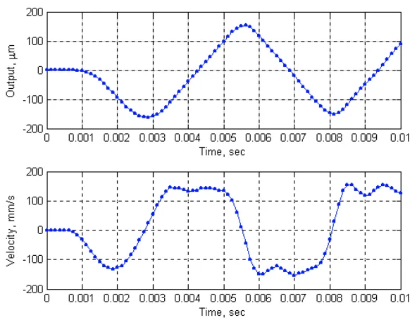
ANGE

(63)

Figure 4-1. FTS response associated with a 200 Hz, 300µm P-V input signal and its velocity

(64)

Output

(a) Shape of the FTS response and its frequency (b) Assembly of the frequency components with

spectrum respect to the FTS output

Figure 4-2. Frequency analysis of the distorted output trajectory

(65)

Figure 4-3. 3D frequency response as a Figure 4-4. Operating range of the Variform function of input amplitudes

4.2 D

YNAMICS OF THE

V

ARIFORM

P

OSITION

S

ENSOR

(LVDT)

The Variform FTS uses an LVDT as a position sensor that closes the feedback loop of its tracking controller. To eliminate disturbances in the measurement, the displacement measuring system implements an internal filter that, however, modifies the dynamic response of the monitored axis motion. Therefore, the tool path measured by the LVDT cannot be used for the FTS dynamics measurement technique in Section 3.2. To this end, the actual tool motion was measured with an external capacitance gauge (Lion Precision) placed in front of the tool holder, whose bandwidth is much higher than the LVDT’s. Time-based signals of the Variform axis position measured by the LVDT and the capacitance gauge are

displayed on a monitor as shown in Figure 4-5. The actual path was delayed by 21° with

(66)

gauge that was determined using the same measurement technique as the actuator dynamic

response. Note that the phase response started at 180° because the two sensors were

measuring in opposite directions. Therefore, the LVDT signal was ahead of the signal of the

capacitance gauge by 18° at 100 Hz. As with the inverse dynamic response of the FTS, the deconvolution algorithm can also compensate for the feedback sensor's dynamic response.

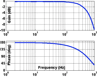
The transfer function showes that the LVDT implements a second order filter with 500 Hz bandwidth where the amplitude dropped off by 0.707 (of 3 dB) and a filtered output signal was 90o out of phase. Another note was that the gain at high frequencies descended about 40 dB over ten increments of the LVDT natural frequency range (500 – 5000 Hz). This implied that the Variform implemented a 2nd order internal filter in its displacement sensor.

Figure 4-5. Phase of the tool motion measured _{Figure 4-6.}_{Dynamic response measured by}

(67)

LVDT dynamics measurement using a laser interferometer

Despite its high bandwidth, a measurement with a capacitance gauge is limited to a small range (± 25µm). It cannot be used to identify the dynamics of the LVDT over the entire

range (± 200µm) of the Variform. Thus, new instrumentation was needed to characterize the response of the Variform’s position sensor. A laser interferometer makes use of a Doppler effect to create interference between two polarized beams. Since resolution of the measurement is proportional to the wave length λ of He-Ne laser (633 nm), it offers a high

accuracy with a long range and a high bandwidth.

4.2.1 Laser operation

A single pass interferometer divides a laser beam which composes of two orthogonal linear-polarization (squares for horizontal and dots for vertical as illustrated in Figure 4-7) into two separate beams. Note that the polarized beams are originally generated with a fixed frequency difference. These polarized beams are then re-combined after directed by a beam-splitter, shifted to circular polarization by ¼ wave plates, reflected by two retroreflectors, and re-shifted to the linear polarization. One polarized beam heads to a stationary, while the other to a moving object, at which Doppler effect modulates the beam frequency and generates interference with the other beam at an external receiver. Afterward, an Axiom 2/20

series interpolates the measurement data to achieve a high resolution of λ1 /256 or 2.47 nm per count.

1 _Α

(68)

Figure 4-7. Single-pass laser interferometer configuration

(69)

An output position data (or an accumulated laser count) of the Axiom 2/20 series is refreshed at the register interface with a constant rate of 10 MHz, but can be read at a rate up to 2 MHz. An access of the position data in this constant data rate mode; as illustrated in Figure 4-8 is to send a sample signal to pause the data transfer between a accumulator and a register interface so that the position data can be transmitted out of the 2/20 series, while the counter still keeps updating the measured position of the moving object. Note the accessed data in a 16-bit unsigned format.

4.2.2 Data acquisition system

This research made use of the dSPACE 1104 series to control the hardware systems, such as a control board of the Axiom 2/20 series, an axes controller of a diamond turning machine, and the Variform FTS, from a model in the MATLAB/simulink module. The dSPACE can access in real-time either analog, digital, or encoder signals, and operate on synchronous or asynchronous tasks from various interrupt sources such as timer chips, software, external sources, PWM interrupts. The interface under the constant data rate mode of the laser interferometer system can be implemented at a fixed sample rate (or a synchronous task) for a measurement of FTS dynamic response.

As the most common scheme for a synchronous task in MATLAB/simulink, a timer interrupt service routine can be used to acquire a measured position data from the Axiom register

(70)

Axiom register interface and also recorded an FTS command signal. Second, since the 2/20 series needs at least 200nsec before the data in the register becomes available, the dSPACE waited for another cycle, then acquired the tool position data. Third, one more cycle delay was needed to release the position held. The Axiom then refreshed new position data from the accumulator to the interface. Since the acquisition sequence took 3 cycles of a 50kHz

sample rate, the position data can be updated every 60µsec.

Figure 4-9. Acquisition the Axiom 2/20 series using the dSPACE

(71)

only a positive number from 0 to 65535 (or 216-1) when converted to a decimal format. The

total count covers only a distance of 161.87µm (65535 counts × 2.47 nm.) The excess

displacement is then wrapped around where the count hits the limit (either 0 or 65535) and starts over at the other end. In Figure 4-11, a position data after the format conversion decreases to zero count and continues its profile from the other end. Consequently, an additional process is needed to smooth the wrapped around position profile so that the unwrapped results can be illustrated as Figure 4-12.

(72)

The result of the measurement agreed with the response observed by the capacitance gauge (in Figure 4-5); the actual tool trajectory had less attenuation and smaller phase lag than what the LVDT displays.

Figure 4-11. A wrapped around profile of a swept sine wave

Figure 4-12. An unwrapped profile of the FTS motion with respect to the desired and the

(73)

The format conversion and the unwrap operation can be proceeded in real-time using the dSPACE. The adjusted position data is then transferred to the Stanford spectrum analyzer to determine the dynamic response of the FTS as shown in a schematic in Figure 4-13.

Figure 4-13. Data flow of the FTS dynamics measurement using a laser interferometer

(74)

a) Gain response of the LVDT

b) Phase response of the LVDT

(75)

4.3 N

ONLINEAR

C

HARACTERISTICS OF

T

HE

V

ARIFORM

FTS

To shape its characteristics to a linear system, the Variform FTS implements a reference capacitor loop to deal with inherent hysteretic behavior of the PZT driving system, constructs a feedback controller to reduce influences of disturbances, and integrates additional filters. Nevertheless, the actuator still exhibits nonlinearly response to varying amplitude input command signals.

Figure 4-15. Nonlinearity of the Variform to various amplitudes of input command signals

(76)

combined with large amplitudes. The pre-compensation for the FTS dynamics now becomes more complicated since the response is not only a function of frequency, but also a function of amplitude. While the input amplitude is growing, the peak of the gain response at the

natural frequency is decreasing. The peak of the gain response associated with 80µm P-V

amplitude is 1.16 at 200 Hz whereas the peak associated with 240µm P-V is only 1.05 at 130

Hz. Note that the established operating range (in Figure 4-4) eases this complication by avoiding conditions when the velocity of a command exceeds the physical limits of the FTS.

4.3.1 Gain scheduling scheme for 3D deconvolution

When a desired machined surface is a non-rotationally symmetric (NRS) feature such as torics, the tool trajectory occasionally displaces in aperiodic manner, and changes its amplitude at least once a revolution. A tool excursion of a toric feature is the square of a sine wave with twice the frequency of the revolution. Its amplitude is linearly decreased as the tool moves toward the center. To modify such a desired excursion with the inverse dynamics algorithm, the transfer function associated with the appropriate amplitude must be selected. To this end, the nonlinearity of the Variform FTS was investigated with a series of modified input command signals which pre-compensate for the responses of different amplitude. Then, the actual excursion that matches the desired path became the basis for the amplitude selection scheme.

In Figure 4-16, a full-period of a 240µm P-V (or 12 volts P-V) cosine wave with a frequency

(77)

desired excursion for a nonlinearity test, and modified into different input command signals

using the dynamic responses associated with the input amplitudes from 80 to 380µm P-V.

The modified input signals associated with small amplitude of 80 and 160µm P-V resemble

each other while the remainder had bigger amplitude and more leading phase angles. This means that the selection of the appropriate dynamic response is critical when the desired trajectory has large amplitude (great than 160µm P-V.)

Figure 4-16. Amplitude dependent modified input signals

Since the dynamic response measurement makes use of sinusoids to determine the dynamic characteristics of a system, it is reasonable to base a modified input command for a cosine wave on a value equal to the magnitude. Consequently, the series of the modified input

(78)

The operation was performed in MATLAB resulting in a series of the simulated output trajectories

Figure 4-17 illustrates the path differences of the modeled output paths with respect to the desired excursion. Since the dynamic response canceled out with its inverse, the path

difference of 240µm P-V was a flat line (a solid line). The differences of the gain and phase response influenced the degree of the path difference. In particularly for the amplitude of

380µm P-V, the path difference (a dotted line) was 60µm P-V or a quarter of the amplitude

of the desired excursion.

Figure 4-17. Influence of the nonlinearity to the path differences with respect to the desired

(79)

The Variform FTS was commanded to displace a tool axis in the air while mounted on an optical table using a series of modified input command signals. As expected, it appeared that

the transfer function of the 240µm P-V yielded a close match to the desired trajectory. In Figure 4-18, the actual tool trajectories (x marks) was identical to the desired path (a solid line) except at the transition from a sinusoidal profile to a flat line. The path difference was limited at 2µm P-V for the most part of the cosine wave. At the edges, the difference was

less than 10µm. Thus, the gain scheduling scheme will select a transfer function associated with the amplitude of the desired tool path for the inverse actuator dynamics algorithm.

Figure 4-18. Comparison of the desired and the actual tool trajectory associated with the

(80)

CHAPTER 5 BLOCK DECONVOLUTION

The preceding chapters have shown the potential of a deconvolution algorithm that can pre-compensate the dynamic response of an actuator to reduce form errors in a machined part. The amplitude of the tool excursion was scaled and its phase was shifted forward to account for gain and phase response of the actuator [16]. However, as discussed in Section 4.3, the Variform FTS has a different gain response to various amplitudes of input signal. Accordingly, the modification of a whole tool trajectory with one dynamic response may not correctly produce a non-rotationally symmetric (NRS) surface whose the depth-of-cut is changed at particular r and θ.

Error Compensation Using Inverse Actuator Dynamics

ABSTRACT

ERROR COMPENSATION USING INVERSE ACTUATOR DYNAMICS

BIOGRAPHY

ACKNOWLEDGEMENT

TABLE OF CONTENTS

LIST OF TABLE

LIST OF FIGURES

CHAPTER 1

INTRODUCTION

1.1 D

T

F

T

S

X

Z

θ

w

1.2 NRS F

1.2.1 Static Decomposition

1.2.2 Dynamic Convolution

1.3 R

L

1.4

O

O

T

R

1.5 O

D

CHAPTER 2

CONVOLUTION AND DECONVOLUTION

2.1 L

, T

-I

S

∑

∑

∑

∑

2.2 D

S

P

(DSP)

2.2.1 Analog to Digital Conversion

t

=

n

δ

t

y(t)

t

y[n

δ

t]

n

δ

t

2.2.2 Sampling Theorem

[ ]

(

(

)

)

( )

∑

2.2.3 Superposition

2.3 I

R

2.4 C

[

]

[ ]

[ ]

[ ]

∑

[

[ ]

]