Development of MEMs Micro-Bridge Mechanical Resonators Interrogated By Microcavity Interferometry

(1)

ABSTRACT

SHELTON, WILSON ANDREW. Development of MEMs Micro-Bridge Mechanical Resonators Interrogated By Microcavity Interferometry. (Under the direction of Leda M. Lunardi and John F. Muth.)

Miniature resonators such as microelectromechanical systems (MEMS) cantilevers

have found multiple uses including development of mass resonant sensing. In this thesis, by

the microcavity interferometer technique, we investigate the properties of bulk

micromachined silicon nitride membranes that are wafer bonded to a substrate to form a

Fabry-Perot cavity.

Photothermal actuation is used to drive the motion of the bridges by frequency

modulating a 980nm diode laser, while the shift in Fabry-Perot resonance is detected by

monitoring the intensity using of a continuous wave 1550nm tunable laser. Using this

technique, 100 femtometer deflections can be easily monitored.

A variety of double clamped beam structures were investigated as a function of beam

width and length. Depending on the dimensions of the micro-bridges, resonance frequencies

from 10kHz to 5MHz were observed. For smaller bridges of dimensions 30μm length and

10μm width, resonance frequencies near 1MHz, quality factors of Q ~ 150 were observed in

air at room temperature. However in vacuum, the quality factors on the order of Q ~ 7000

were observed, verifying air damping as the main source of energy loss.

Moreover, in air at room temperature, the Brownian motion of the bridge was

observable without any photothermal driving force suggesting the possibility of using this

structure as an un-powered chemical sensor and demonstrating the sensitivity of the optical

(2)

The sensitivity of the bridge to chemical exposure was not quantified, but

environmental perturbations were observed to change the resonant frequency of the bridge by

(3)

DEVELOPMENT OF MEMS MICRO-BRIDGE MECHANICAL RESONATORS INTERROGATED BY MICROCAVITY INTERFEROMETRY

by

WILSON ANDREW SHELTON

A thesis submitted to the Graduate Faculty of North Carolina State University

in partial fulfillment of the requirements for the Degree of

Master of Science

ELECTRICAL AND COMPUTER ENGINEERING

Raleigh, North Carolina 2006

APPROVED BY:

________________________________ Leda M. Lunardi

Chair of Advisory Committee

_________________________________ John F. Muth

Co-Chair of Advisory Committee

(4)

BIOGRAPHY

Wilson Andrew “Andy” Shelton was born in Martinsville, Virginia on November 10,

1981 and grew up in Stoneville, North Carolina. He attended Dalton L. McMichael High

School where he played football, basketball, and baseball. After graduating high school in

June 2000, he attended Wake Forest University. While there, he played on the football team

and participated in undergraduate research in the physics department. This research dealt

with optical trapping and micromechanics, in both of which he took great interest. His

undergraduate research honors thesis, entitled “Nonlinear Motion of Optically Torqued

Nanorods” was published in Physical Review E in March 2005. After receiving his

Bachelors of Science degree in Physics from Wake Forest in May 2004, he attended North

Carolina State University to pursue graduate work in Electrical Engineering. While there, his

thesis research was an optical MEMS project which was a perfect fit considering his optics

and micromechanics background. He was married on July 29, 2006 to his high school

sweetheart Katherine Leigh Morrison. He received his Masters degree in Electrical

(5)

ACKNOWLEDGEMENTS

I would first of all like to thank Dr. Leda Lunardi for taking me under her wing and having the faith to let me work with her. Her support for me as a graduate student is greatly

appreciated.

I also want to thank Dr. John Muth for letting me work a great project which really utilized by previous experiences. While always working with a large group of graduate students, he always found time to help me with or talk to me about this project any time. His enthusiasm and willingness to give a hand in the lab made this project quite enjoyable.

The amount of help that Joe Matthews put into this project can never be quantified. His assistance in the clean room was always valued, whether assisting with the equipment or simply answering fabrication questions.

I want to thank Dr. David Nackashi for always being both a knowledgeable source of information and a source of stress-relieving humor. Whether wanting some information about silicon nitride membranes or a quick cheap laugh, David was always the guy with which to talk.

A special thanks goes out to Jonathan Holland whose modeling was very helpful in understanding the mode structures of the devices created.

I want to send special thanks out to a few guys in Dr. Muth’s group. I want to especially thank Jason Kekas, Anuj Dhawan, and Patrick Wellenius for being great friends. They each were always willing to drop anything to help if the need arised and their friendship,

assistance, and lunchtime appetites were always appreciated.

(6)

LIST OF TABLES

Table 2.1 – Real and imaginary refractive indices of aluminum ... 26

Table 2.2 - Table showing thickness and refractive index of each layer... 28

Table 3.1 – Various material properties used in the resonant frequency analysis ... 36

Table 3.2 - Various constants associated with the first four transverse modes ... 37

(9)

LIST OF FIGURES

Figure 1.1 – General structure of a chemical or biological sensor ... 2

Figure 1.2 – A change in the Stokes shift denotes a change in the concentration ... 4

Figure 1.3 - A broadband source sends light into a multipass sealed Herriott cell... 5

Figure 1.4 - A surface plasmon resonance based sensor ... 6

Figure 1.5 - An interference method based sensor ... 7

Figure 1.6 - Schematic showing the mass-loading technique... 8

Figure 2.1 – The optical beam deflection technique... 14

Figure 2.2 - Laser Doppler vibrometry schematic. ... 15

Figure 2.3 - Net reflectance of an ideal Fabry-Perot interferometer... 18

Figure 2.6 - Plot of real and imaginary refractive indices of aluminum... 26

Figure 2.7 - Each layer in the stack for the analysis ... 27

Figure 2.8 - Plot of net reflectance (using transfer matrix method)... 28

Figure 2.9 - Plot of the net reflectance (using transfer matrix method)... 29

Figure 2.10 - Plot of the net reflectance (using transfer matrix method)... 30

Figure 3.1 - Simple model of a double-clamped beam. ... 34

Figure 3.2 – Double log scale plot of the theoretical fundamental resonant frequency ... 36

Figure 3.3 - Deflected double-clamped beam... 39

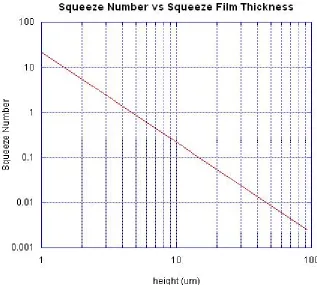
Figure 3.4 - Double log scale plot of the squeeze number... 41

Figure 3.5 - Squeeze inertia number and squeeze damping number ... 42

Figure 3.6 - Plot of the Q factor as a function of the squeeze film thickness ... 43

Figure 3.7 - Plot of the relative frequency as a function of the squeeze film thickness ... 44

Figure 3.8 – Frequency spectrum of dissipation-induced amplitude noise ... 47

Figure 4.1 - Image of a piece of silicon which has been anisotropically etched ... 50

Figure 4.2 - Visible and Near Infrared Transmittance of Silicon Nitride ... 51

Figure 4.3 - Infrared Transmittance of a 200nm thick layer of Silicon Nitride... 52

Figure 4.4 – The membrane creation process ... 55

Figure 4.5 - A top-view of a silicon nitride membrane... 56

(10)

Figure 4.7 - Schematic of the wafer after the RIE process ... 58

Figure 4.8 - Image of 1000μm long silicon nitride double-clamped beams ... 58

Figure 4.9 - Plot of the percent transmission for 2mm thick Borofloat® plate glass. ... 59

Figure 4.10 - Plots of the bonding strength of various patternable materials ... 60

Figure 4.11 - Image of a simple microcavity... 60

Figure 4.12 – Shape of bonding pad created with the SU-8 ... 61

Figure 4.13 – Image of a completed device... 62

Figure 5.1 - The HP 8168F C-band tunable laser ... 64

Figure 5.2 - The fiber coupler plus the 980nm pigtail laser source ... 65

Figure 5.3 - Schematic of the optical interrogation setup... 66

Figure 5.4 - Image of the optical interrogation setup... 68

Figure 5.5 - Screenshot of the front end of the LabView code... 69

Figure 5.6 - Image of the Tektronix oscilloscope. ... 70

Figure 5.7 - Image of the Agilent E5100A network analyzer... 71

Figure 5.8 - Screenshot of the front end of the LabView code... 72

Figure 6.1 – Devices tested... 75

Figure 6.2 – SEM image of 30μm long, 5μm wide bridges... 76

Figure 6.3 – SEM images of bridges ... 76

Figure 6.4 - Scans at center of 50μm long bridges of various widths... 77

Figure 6.5 – Plots of the frequency response... 79

Figure 6.6 – Plots of the frequency response of 30μm, 40μm, and 50μm wide bridge ... 80

Figure 6.7. By taking scans along lines a,b,c, and d ... 82

Figure 6.8 – Schematic of a 120μm long 50μm wide bridge... 83

Figure 6.9 – Series of ten scans along width of 120μm long 50μm bridge ... 83

Figure 6.10 Drawing of the transverse fundamental mode... 84

Figure 6.11 – Series of scans along length of 120μm long 50μm wide bridge. ... 84

Figure 6.12 – Fundamental Resonant Frequency of 10μm wide bridges ... 85

Figure 6.13 - Fundamental Resonant Frequency of 50μm wide bridges. ... 86

Figure 6.14 – Fundamental Resonant Frequency of 120μm Long Bridgs... 87

Figure 6.15 – Linear scale frequency response of 120μm long bridges. ... 88

(11)

Figure 6.17 – Log scale frequency response of the unclamped transverse mode... 90

Figure 6.18 – Relationship between the resonant frequency and interrogation laser power. . 91

Figure 6.19 - Quadratic dependence of signal amplitude on the interrogation laser power. .. 91

Figure 6.20 - Shift in the resonance as the driver laser diode current is varied... 92

Figure 6.21 - Relationship between frequency and 980nm driver laser diode current. ... 93

Figure 6.22 - Relationship between amplitude and the 980nm driver laser diode current. .... 93

Figure 6.23 – Resonant frequency as a function of the wavelength ... 94

Figure 6.24 – Resonant frequency vs. time as illumination lamp is powered off and on... 95

Figure 6.25 – Pressure chamber connected to a dry vacuum pump... 96

Figure 6.26 – Plots of resonance in air (left) and vacuum (right)... 97

Figure 6.27 – Mechanical quality factor as a function of chamber pressure. ... 97

Figure 6.28 – Noise spectrum of an un-driven bridge ... 98

Figure 7.1 – Employing ball lens to create microcavity. ... 101

Figure 7.2 – Employing a fiber-based system to create Fabry-Perot microcavity... 102

Figure 8.1- Mask used to create the membrane arrays ... 104

(12)

1 OPTICAL ELECTRONIC NOSES

1.1 Introduction

All living organisms from bacteria to humans respond to chemicals in the

environment. In more developed organisms such as animals and humans, chemicals are most

often detected by using the taste or olfactory senses. The human sense of smell is a very

sensitive system able to respond for some compounds at parts per billion (ppb)

concentrations. However it is unreliable because it can vary between different noses from nil

to highly sensitive1.

The need to detect deadly explosive or chemical agents has become very important

for homeland security and defense applications. While explosive agents may not be

detectible by the human noses, animals such as dogs and rats have been used successfully to

perform the detection task, requiring sophisticated handling and training besides the short

lifetime. Among the most toxic and rapidly acting of the known chemical warfare agents are

nerve agents such as sarin gas, so human and animals noses would not be used to detect these

agents. Another alternative is to use a mechanical olfaction system.

The generalized detection of volatile organic compounds (VOCs) is most often

referred to as electronic nose technology. The electronic nose has generally been based on

(13)

Figure 1.1 – General structure of a chemical or biological sensor. The transducer produces a signal response when the analyte binds to the selective layer.

The first artificial nose created by Persaud and Dodd used semiconductor transducers

to detect various chemicals2. There are currently several electronic nose sensor

technologies3. Included are metal oxide and conducting polymer sensors, both of which use

conductivity as the principle of operation. There are also quartz crystal microbalances and

surface acoustic wave sensors which work on piezoelectricity. Metal Oxide Substrate Field

Effect Transistor (MOSFET) electronic noses use capacitive charge coupling as a means of

detecting gases. Gas chromatography, mass spectrometry, and light spectrum sensors rely on

molecular spectra, atomic mass spectra, and transmitted light spectra respectively. The

ultimate electronic nose sensor technology is the optical sensor which could work in a variety

of methods. Optically based artificial noses have only been introduced in the last few years.

Much advancement in optics in the last fifty years, including lasers, laser diodes,

light-emitting diodes, optical fibers, and very sensitive optical detectors have led to the

ability to sense trace gases optically. An optical sensor is a device that measures change in

one of the properties of light: absorbance, fluorescence, polarization, refractive index,

(14)

components: a light source to interrogate the sensor, optics for directing the light to/from the

sensor, a detector to measure the light from the sensor, and the sensor itself1.

1.2 Optical Sensing Methods

There are five methods of optical vapor sensing: luminescent methods, colorimetric

methods, surface plasmon resonance methods, interference and reflection based methods, and

finally mass-loading methods1. Luminescence is among the most popular method of optical

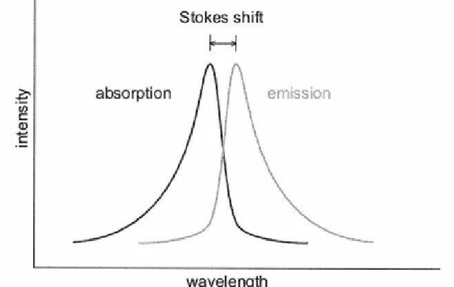
vapor sensing4. Fluorophores are molecules that absorb light at one wavelength and emit

light at another longer wavelength. Photoluminescence is a type of electromagnetic

spectroscopy that uses a beam of light, usually in the ultraviolet wavelengths, to excite the

electrons in molecules of certain compounds to emit light of a lower energy. This lower

energy emission is often in the visible spectrum. This change in absorption and emission

wavelength is referred to as a Stokes shift and the size of this shift represents the energy lost

by the fluorophore during absorption, as shown in Figure 1.2. The efficiency of photon loss

after absorption is referred to as the quantum yield. Luminescence is a popular means of

sensing because of high quantum yields, large separation between excitation and emission

wavelengths, and its intrinsic sensitivity. One example of the mechanisms by which the

fluorophores work is twisted intramolecular charge transfer (TICT). These fluorophore

molecules are designed to be highly polarized in the excited state. When the excited states

(15)

Figure 1.2 – A change in the Stokes shift denotes a change in the concentration of analyte vapors present when bound to the fluorophores.

The second method of optical vapor sensing is the colorimetric method5,6.

Colorimetric sensors measure a change in absorbance or refractive index resulting from

indicator color changes. They rely on changes in the color of an organic sensing material.

These can be small colored beads placed at the ends of an optical fiber bundle, or colored

spots on a chip imaged by a camera. Another type of colorimetric sensor employs a

multi-pass absorption cell such as in the schematic shown in Figure 1.3. Gas is pumped into the

cell which is a gas-tight two mirror cell and allows multiple reflections of laser light, much

like a laser cavity. During these multiple passes, certain wavelengths are absorbed by the gas

molecules and a spectrometer is able to detect these absorbed wavelengths. The input beam

is directed into an iris in one sealed face of the cell and after multiple reflections the beam

exits from the same iris located at the bottom of the left face of the cell in Figure 1.3. From

the absorbed wavelength and the intensity of the output signal, some quantification of the

(16)

Figure 1.3 - A broadband source sends light into a multipass sealed Herriott cell which contains the gas to be analyzed. The output light is sent to a spectrometer where adsorption wavelengths can be detected.

The next type of sensing method is surface plasmon resonance based sensing7. This

technique uses the free conducting electron gas found at the surface of conductive metal

films such as gold and silver. If the interface between two media of differing refractive

indices is coated with a thin layer of gold, the intensity of monochromatic reflected light

decreases at a precise, resonant incident angle. This surface plasmon resonance is due to the

resonance energy transfer between evanescent wave and surface plasmons. The resonance

conditions, specifically angles and wavelengths, are influenced by the material adsorbed onto

the thin metal film. The resonant angle is dependent upon the refractive index of the

dielectric medium, so any changes in refractive index at the surface, caused by the absorption

of vapor molecules into the chemoselective polymer on the surface, can be monitored in real

time by measuring the value of the resonant angle as shown in Figure 1.4. Some drawbacks

of the surface plasmon resonance method are that it is not very sensitive and the response and

(17)

Figure 1.4 - A surface plasmon resonance based sensor. With no analyte vapors present, the incoming beam experiences a reflection minima at a particular angle (solid line). The angle of minimum reflection shifts (dotted line) as the analyte vapor is captured and adheres to the sensor surface.

Interference and reflection based methods employ reflectometric interference

spectroscopy (RIfS)8. Some polymeric films when exposed to specific chemical vapors

experience a large change in optical thickness. The films also experience a change in

refractive index, but the index change is quite small relative to the optical thickness change.

This technique which uses light incident at the interface of two planar optical layers is known

as reflectometric interference spectroscopy. The light reflects from both the top and bottom

of the film, setting up an interference pattern that is very sensitive to changes in the optical

thickness of the polymer sensing film, as shown in Figure 1.5. The adsorption of the analyte

vapors onto the surface gives rise to shifts in the Fabry-Perot interference fringes, which can

be detected with a spectrometer. Also, one can monitor the emission at a specific wavelength

and observe the sharp decreases in intensity as the interaction with the analyte vapors takes

(18)

Figure 1.5 - An interference method based sensor. When a vapor analyte is adsorbed into the top layer, the optical thickness of the body changes thus producing a shift in the interference fringes.

The final method of optical vapor sensing is referred to as mass loading9,10,11,12,13,14.

This method makes use of resonating microcantilever transducers, much like what is used on

an atomic force microscope (AFM) for molecular level imaging. In mass loading, the

cantilever transducers are coated with a polymeric film which reacts with a specific analyte

vapor. As the analyte vapors contact the polymeric film on the cantilever, the mass and/or

strain of the cantilever could change. The general idea behind these sensors is that the

physical, chemical, or biological stimuli are able to affect the mechanical characteristics of

the resonating transducer so that the change can be detected by electrical or optical means.

Many polymeric films today are able to be synthesized so that they react with a single

chemical. These polymeric films remain noble until the chemicals contained within the gas

to be detected come into contact with the sensor. The selectivity of these polymers removes

some uncertainty in the detection process. They can be chosen to detect specific airborne

hydrocarbons or discern between humidity and other similar polar molecules. The

(19)

detected. This change in mass or strain as the analyte vapors are adsorbed can be detected

optically by measuring the deflection of an incident laser beam, as shown in Figure 1.6. This

deflection could be a static deflection in which the adsorption simply causes the cantilever to

bend or the deflections could also be dynamic in scope, where the frequency at which the

cantilever is oscillating is the measured quantity. As the analyte vapors adsorb onto the

cantilever in this method, the added mass and variation of strain will produce a shift in the

resonant frequency of the cantilever.

Figure 1.6 - Schematic showing the mass-loading technique. The analyte vapors change the mechanical properties of the cantilever which causes a shift in the resonant frequency at which the cantilever oscillates.

This optical method of detecting a change in the resonant frequency is the method

used in this research. Cantilever transducers continue to improve as methods of chemical

sensing because of the ever-changing and improving technology. As the size of MEMS

devices continues to decrease, the ability to detect smaller masses become a definite

possibility. The mass loading/resonant cantilever platform was chosen because of the

continuing areas of improvement due to technological advancements in MEMS fabrication

(20)

1.3 Goals of This Research

Most chemical sensors require a great deal of signal processing and amplification at

the source besides having a large area and lots of interconnects1. This project uses an

optical-based chemical sensor that is a micromachined Fabry-Perot microcavity. The goal is

to build sensors that are able to be remotely modulated and interrogated without any

electrical connections or signal processing at the sensor level by both modulating the signal

and directing that modulated light back to the detector. Remote interrogation will make this

type of sensor much safer to use as a means of detecting deadly gases.

Silicon nitride is the material of choice for the cantilever in this project. This material

is attractive because it has been used for many years in atomic force microscope (AFM)

probes with pre-existing technology and knowledge as a resonator.

Chapter 2 includes the use of optical micro electromechanical systems (MEMS)

interferometry as a technique for detecting small mechanical deflections, discussing the

basics of Fabry-Perot interferometry and how small mechanical deflections are used to

change the interference characteristics of the device.

In Chapter 3, the mechanical theory of the double-clamped beam is presented. This

analysis includes the material properties of silicon nitride, the Euler-Bernoulli theory of

motion for the double-clamped beam, and the effects that air damping has on its motion.

Thermal-mechanical noise within the system is also discussed.

In Chapter 4, the steps to fabricate the devices are given in detail. From the bare

double-side polished silicon wafer, the final 1cm2 chips contained over 800 double-clamped

(21)

In Chapter 5, the setup for optical interrogation and data acquisition are presented.

The setup includes light sources, fiber and free space optics, detection devices, network and

spectrum analyzers, and data acquisition routines.

Chapter 6 is devoted to the analysis and discussion of the experimental results. Data

for characterization included resonant frequency measurements as functions of bridge length

and width as well as clamped and unclamped mechanical modes. The effects of various

experimental conditions such as source intensity and wavelength on the resonant frequencies

were studied.

(22)

1.4 References

1

T.C. Pearce, S.S. Schiffman, H.T. Nagle, and J.W. Gardner, Handbook of Machine Olfaction: Electronic Nose Technology, KGaA, Weinheim: Wiley-VCH, 2003.

2

K. Persaud And G. Dodd, “Analysis of Discrimination Mechanisms In The Mammalian Olfactory System Using A Model Nose,” Nature, volume 299, pp.352-355, Sep. 1982.

3

H.T. Nagle, R. Gutierrez-Osuna, S.S. Schiffman, “The How and Why of Electronic Noses,” IEEE Spectrum, volume 35, pp. 22-34, Sep. 1998.

4

D.R. Collingridge, W.K. Young, B. Vojnovic, P. Wardman, E.M. Lynch, S.A. Hill, D.J. Chaplin, “Measurement of Tumor Oxygenation: A Comparison between Polarographic Needle Electrodes and a Time-Resolved Luminescence-Based Optical Sensor,” Radiation Research, volume 147, pp. 329-334, Mar. 1997.

5

K.S. Suslick, N.A. Rakow, A. Sen, “Colorimetric sensor arrays for molecular recognition,” Tetrahedron, volume 60, pp 11133-11138, Nov. 2004.

6

P. Werle, R. Mücke, F. D´Amato, T. Lancia, “Near-infrared trace-gas sensors based on room-temperature diode lasers,” Applied Physics B: Lasers and Optics, Volume 67, pp. 307-315, Sep. 1998.

7

B. Liedberg, C. Nylander, I. Lundstroem, “Surface plasmon resonance for gas detection and biosensing,” Sensors and Actuators, volume 4, pp. 299-304, 1983.

8

D. Reichl, R. Krage, C. Krumme, G. Gauglitz, “Sensing of Volatile Organic Compounds Using a Simplified Reflectometric Interference Spectroscopy Setup,” Applied Spectroscopy, volume 54, pp. 583-586, April 2000.

9

G. Y. Chen, T. Thundat, E. A. Wachter, and R. J. Warmack, “Adsorption-induced surface stress and its effects on resonance frequency of microcantilevers,” Journal of Applied Physics, volume 77, pp. 3618-3622, Apr. 1995.

10

N. Lavrik, M. Sepaniak, P. Datskos, “Cantilever transducers as a platform for chemical and biological sensors,” Review of Scientific Instruments, volume 75, pp. 2229-2253, Jul. 2004.

11

A. Clark, L. Whitehead, C. Haynes, A. Kolicki, “Novel resonant-frequency sensor to detect the kinetics of protein adsorption,” Review of Scientific Instruments, volume 73, pp. 4339-4346, Dec. 2002.

12

(23)

13

A. Zribi, A. Knobloch, and R. Rao, “CO2 detection using carbon nanotube networks and micromachined resonant transducers,” Applied Physics Letters, volume 86, 2005.

14

(24)

2 OPTICAL MEMS INTERFEROMETRY

2.1 Introduction

In the past ten years, micromachined Fabry-Perot interferometers have been an area

of extensive development in MEMS processing1,2,3. Some of these include sensing elements

in the form of accelerometers4, microphones5, capacitive switches6, and pressure sensors7,8,9.

They have also found their way into optical communications systems and are being used as

tunable filters in wavelength division multiplexing (WDM) fiber optic systems because of

their ability to be low loss, narrow linewidth, and tunable at low-voltages10. There are

several advantages to using optical interferometry to characterize micromachined systems

including immunity to electromagnetic interference, the non-destructive and non-contact

nature of the measurement, the very high bandwidth limited only by the photodetector

response, and the high precision of the measurement. This section addresses the principles of

microcavity interferometry and how it can be used to detect mechanical motion.

2.2 Optical Detection of Micromechanical Deflections

One main goal of this project is to detect the frequency, amplitude, and phase at

which a driven micromachined beam is vibrating. Several optical methods have been used

for detecting deflections of micromachined devices but the main methods include the optical

beam deflection, laser Doppler vibrometry, and interferometric techniques11. These

techniques allow for interrogation of the sample with no physical contact. In the optical

beam deflection technique12, which is used in atomic force microscopy, a laser beam is

directed at a microcantilever with a mirrored surface. The reflected beam is directed at a

detector called a position sensitive photodetector which consists of four quadrants. The

(25)

from one quadrant dominates and allows the position of the cantilever to be determined.

Figure 2.1 demonstrates how the incident and reflected beams are unable to be oriented along

the same direction in an optical beam deflection setup.

Laser

Reflective Surface Membrane or

Cantilever

Position Sensitive Photodetector

Figure 2.1 – The optical beam deflection technique such as is used in an atomic force microscope.

The advantages of this system are the absence of any bulk electrical connections to

the microcantilever and the simplicity of the design. Some disadvantages of this type of

optical system are that changes in the optical properties of the surrounding material may

cause unwanted refraction of the laser beam. Also, current position sensitive photodetectors

have very low bandwidths on the order of a few hundred kilohertz due to their relatively

large size. Also, incoming and reflected beams cannot be oriented along the same path at

normal incidence when deflections are only along the z-axis. This prevents the transmitter

and receiver from being near each other if interrogated at long distances.

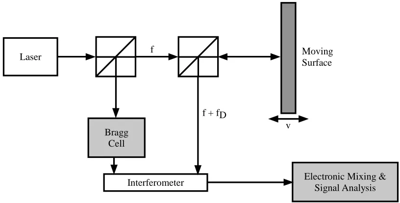
Another vibrometry technique is laser Doppler vibrometry13 which relies on the

detection of a Doppler shift in the frequency of coherent light scattered by a moving target.

(26)

technique does allow for the incoming and outgoing beams to be aligned along the same axis,

but it suffers from many drawbacks. One drawback is that the Doppler shift gives no

information on the static position of the structure. Shown in Figure 2.2, the Doppler

vibrometry information is very dependent on the position of the reference optics and requires

that they be damped and stationary at all times. Any vibration or misalignment of the

reference optics will introduce unwanted noise into the system.

Electronic Mixing & Signal Analysis v

Laser

Bragg Cell

Interferometer f

f + fD

Moving Surface

Figure 2.2 - Laser Doppler vibrometry schematic.

2.3 Optical Microcavity Interferometry

The technique used for this research is an interferometric technique known as optical

microcavity interferometry14,15. Optical microcavity interferometry is a technique which uses

the optical interference between two surfaces as the means of detecting motion. Microcavity

interferometry allows for high-bandwidth, high-resolution measurements of the nanoscale

deflections of the device under test. The interference not only allows for the incoming and

reflected beam to be aligned atop each other, but requires it. The splitting of the incoming

(27)

the need for complex optics. Also any small vibrations of the reference optics have no effect

on the measured properties of the device because all interference depends on the separation

between the two surfaces of the cavity. The microcavity in effect becomes a Fabry-Perot

interferometer which consists of a pair of parallel, partially-reflective surfaces. When light is

incident upon a Fabry-Perot interferometer, the light between the two surfaces interferes and

produces a very characteristic reflection or transmission spectrum. The reflected intensity for

a Fabry-Perot cavity is given by the following equation16:

) / 2 ( sin 4 ) 1 ( ) / 2 ( sin 4 ) ( 2 2 1 2 2 1 2 2 1 2 2 1 2 λ π λ π nd R R R R nd R R R R E E R i r net + − + − = ⎥ ⎦ ⎤ ⎢ ⎣ ⎡

= (2.1)

where Er and E are the reflected and incident electric fields, i R1 and R2 are the reflectances

of each plate, n is the index of the material between the plates, d is the separation between

the plates, and λ is the wavelength of the incident beam. There are many interesting details

about this equation which can and must be analyzed for use in the interferometer. These

include the effect each variable in the above equation has on the resulting spectrum. The

effect of different reflectance values are addressed in the analysis including whether or not

the reflectance values of each surface be the same and if so, how high those reflectances

should be. The optimal plate separation is addressed based on the tunability of the laser

source and finally, the effect a changing or oscillating plate separation has on the spectrum is

also addressed.

2.4 Effects of Variables on Fabry-Perot Spectrum

The following section uses several plots to show the effect each variable within the

Fabry-Perot equation has on the reflection spectrum, including the reflectances R₁ and R₂

(28)

1625nm. The appropriate plate separation based on the wavelength separation between each

resonance of the curve is given by the following equation

λ λ

Δ =

n d

2 2

(2.2)

where λ is the center wavelength between the peaks, n is the index of the cavity material,

and Δλ is the wavelength separation between each peak. For the 100nm tuning range of the

laser centered at 1575nm, the minimum plate separation needs to be 12.4μm in order to see at

least one resonance over that tuning range. For simplicity, each of the following analyses

assume a cavity separation of 15μm. Another equation relating the plate separation to the

spectral location of each resonant minima is given by the following:

1 2

+ =

j nd j

λ

(2.3)

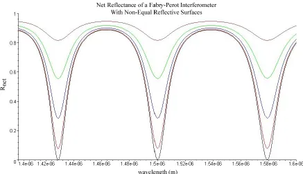
for j=0, 1, 2, …. Each of these resonant minima occurs when the argument of the sin

function within the net reflectance equation equals any multiple of π. The plot in Figure 2.3

(29)

Figure 2.3 - Net reflectance of an ideal Fabry-Perot interferometer considering non-equal reflective surfaces. From top to bottom, the respective reflectances are [R1,R2] = [0.1,0.9], [0.2, 0.8], [0.3,0.7], [0.4, 0.6], and [0.5, 0.5]. The plate separation d=15μm and index n=1.

When the reflectance of each plate is matched, the reflection minimum is zero.

Therefore, matching the reflectance values of each surface is necessary to achieve the

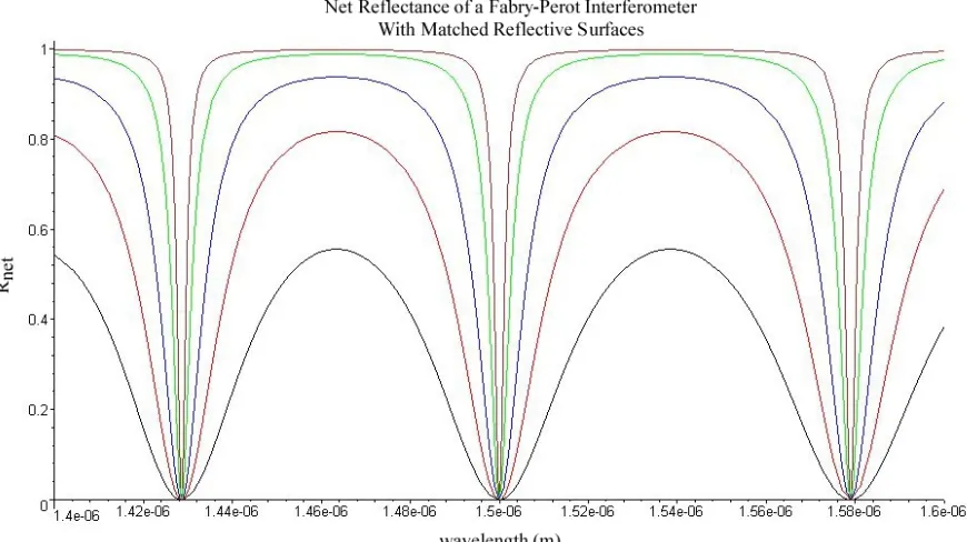
difference between the maximum and minimum values. The plot in Figure 2.4 demonstrates

(30)

Figure 2.4 - Net reflectance of an ideal Fabry-Perot interferometer with identical reflective surfaces (R1=R2). From top to bottom, the respective reflectances are R =0.9, 0.8, 0.6, 0.4, and 0.2. The plate separation d=15μm and index n=1.

As the reflectance values of each face increase, the reflection maximum gets closer to

one. For very high reflectance values, the slope of the curve at each resonance increases

dramatically. Having a sharp slope is very important in terms of sensor sensitivity as will be

discussed later. The term characterizing the sharpness of each optical resonance is known as

the finesse. Assuming the reflectances of each surface are equal, the finesse of a Fabry-Perot

interferometer is given by the following equation:

2 ) 1 (

4

2 R

R F

− =π

(2.4)

where R is the reflectance of each face of the etalon. There are many factors which can have

a detrimental affect on the effective finesse of a cavity. These include spherical bowing,

surface roughness, and departure from parallelism/tilt17,18,19. The overall defect finesseND is

(31)

2 2 2 3 7 . 4 2 1 ⎟ ⎟ ⎠ ⎞ ⎜ ⎜ ⎝ ⎛ + ⎟ ⎠ ⎞ ⎜ ⎝ ⎛ + ⎟ ⎠ ⎞ ⎜ ⎝ ⎛ = λ δ λ δ λ

δ s G P

D

t t

t

N (2.5)

where δts, δtG, and δtP are measures of the spherical bowing, surface roughness (RMS

deviation) and tilt respectively. The resulting overall cavity finesse NE is given by

2 2 1 1 1 F N N D E +

= (2.6)

where F is the finesse derived from Equation 2.4. In the case of this research, the main

defect to worry about was the tilt. To keep the tilt defect finesse factor from dominating the

overall effective finesse of the cavity, the reflectance values were kept low enough so that the

reflectance finesse F dictated the finesse. The tilt was often very apparent because of the

effect a small change in cavity separation had on the Fabry-Perot spectrum. The spectral

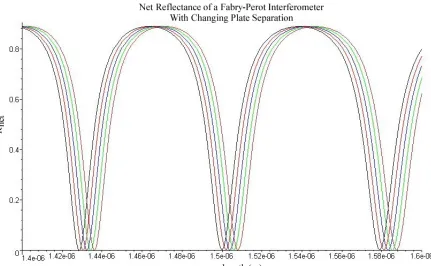
location of each resonance changes with the cavity separation. The plot in Figure 2.5 shows

(32)

Figure 2.5 - Net reflectance of an ideal Fabry-Perot interferometer with changing plate separation. From left to right, the plate separation d=15μm+j20nm with j=0, 1, 2, 3, and 4 respectively. The reflectance values are R1=R2=0.5 and n=1 for simplicity.

As the cavity separation increases, the spectrum makes a shift to the right. If the

mode index j is known from Equation 2.3, the following equation gives an exact value for the

spectral shift due to a change in cavity separation Δd:

d j

n

j Δ

+ = Δ

1 2 λ

(2.7)

The most important things learned from the above equations and plot analyses are that the

reflectances of each face need to be matched and also fairly high. The reflectance cannot be

made too high because a small beam deflection or misalignment would lead to the resonant

minimum being moved easily off of the set interrogation laser wavelength. Though the

above net reflectance equation for a Fabry-Perot interferometer is based on ideal boundary

conditions and only two partially reflective surfaces, practical applications do not involve

(33)

2.5 Transfer Matrix Method

Practical problems usually involve waves propagating in bounded regions in which

different stratified media may be present, and require that account be taken of the

complicating effects at boundary surfaces. Typical boundary surfaces lie between regions of

different permittivities, conductivities, or permeabilities. When an electromagnetic wave

comes into contact with a boundary, part of its energy is reflected back into the incident

medium and the rest of the energy is transmitted through to the next medium. Using

Maxwell’s equations with the appropriate boundary conditions, mathematical expressions for

these reflected and transmitted waves can be found. For both simplicity and practicality of

the application, only waves at normal incidence on planar interfaces will be considered in

this analysis.

The following analyses use the matrix method to describe wave propagation in

stratified media. The stratified media in this analysis are layers in which the properties are

constant throughout each plane perpendicular to the optical axis of propagation. Some

applications of stratified media include antireflection coatings, dielectric mirrors, chromatic

filters, and beam splitters. An analysis by Born and Wolf20 uses Maxwell’s equations to

derive a 2x2 matrix method for determining the net reflectance and transmission of a stack of

stratified media. A 4x4 matrix method by Berreman21 would also work but is unnecessary

due to the polarization independence of the stratified layers. The following describes the 2x2

transfer matrix method and in turn a wavelength-dependent reflectance of the stack of media

used in this experiment is determined.

Derived from Maxwell’s equations, the characteristic matrix of a stratified medium is

a convenient method of expressing solutions to those equations. Born and Wolf find a

(34)

analysis, only the transverse electric waves are considered. The following equations are for a

homogenous dielectric film. The refractive index n is given by the following equation:

r r

n= ε μ

(2.8)

where ε_r is the relative electric permittivity and μ_r is the relative magnetic permeability.

Another value used in the analysis is p given by the following equation:

) cos(θ μ ε r r p= (2.9)

where θ is the angle of incidence for the wave with respect to the normal of the stack. For a

film at normal incidence (θ =0) and relative magnetic permeability 1, the variable p and the

refractive index n are equal. There are no magnetic materials used in this experiment so for

all films in the stack, μr =1. Also, the wave number for a dielectric film is given by the

equation 0 0 2 λ π ω ₌ = c k (2.10)

The 2x2 characteristic matrix for a TE beam in a layer of thickness d is given by the

following equation. ⎥ ⎥ ⎦ ⎤ ⎢ ⎢ ⎣ ⎡ − − = )) cos( cos( )) cos( sin( )) cos( sin( )) cos( cos( 0 0 0 0 θ θ θ θ nd k nd k ip nd k p i nd k M_TE (2.11)

The characteristic matrix for the jth film in which the electric permittivity ε and the magnetic

permeability μ are assumed constant in the layer, the characteristic matrix is given by

(35)

The overall characteristic matrix for a number of stratified media packed together is found by

multiplying the characteristic matrix of each layer together to yield the overall characteristic

matrix, given by the following relationship

∏

₌ = n j j M M 1 (2.13)

The reflection and transmission coefficients are given by the following equations

) ( ) ( ) ( ) ( ' 22 ' 21 0 ' 12 ' 11 ' 22 ' 21 0 ' 12 ' 11 f f f f p m m p p m m p m m p p m m r + + + + − + = (2.14) ) ( ) ( 2 ' 22 ' 21 0 ' 12 ' 11 0 f f p m m p p m m p t + + + = (2.15)

where m_ij' is the i,j element of the characteristic matrix, p is the p-value for the incident ₀

medium (before the stack) and p is the p-value for the terminating medium (after the _f

stack). In terms of r and t , the net reflectance and transmittance for the stack is given by

the following equations

2 r R= (2.16) 2 0 t p p T = f

(2.17)

2.6 Non-Dielectric Media

This matrix analysis remains valid for non-dielectric media within the stratification.

This matrix method can also be used with thin metallic films by considering the metal film to

have a complex dielectric constant. This can simply be done by replacing the refractive

(36)

2.7 Aluminum Optical Properties

For this experiment, aluminum was chosen as the partial reflector for a number of

reasons. The metal of choice had to possess a number of qualities including a high imaginary

index of refraction, low density, and ease of use. Aluminum had all of these qualities. The

importance of the imaginary index is that a very thin film will produce a large reflectance.

Aluminum is also very easy to apply using an electron beam evaporator. Also because

aluminum is non-magnetic, the p-value for that layer can be replaced with the refractive

index also because the μr for aluminum is very close to one. One negative to aluminum is

its ease of oxidation. The electron beam deposition system used, even though pumped down

to near 10-5 torr, still has enough residual oxygen and water vapor to oxidize the first several

nanometers of the aluminum film. The aluminum oxide layer, a dielectric, thus reduces the

reflectance of the film so the aluminum thickness before and after oxidation must be

considered. The thickness measured by the crystal monitor, the physical thickness and the

metal thickness are all different because of the oxidation process within the chamber. The

thickness of the oxide layer can approach about 10nm if given enough time. This thickness

is taken into account and the thickness of the reflective aluminum is reduced. The

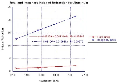
wavelength-dependent refractive index of aluminum was found using data from Ordal et.

al22. The plot in Figure 2.6 gives the real and imaginary indices for aluminum as a function

(37)

Figure 2.6 - Plot of real and imaginary refractive indices of aluminum as a function of wavelength22. Included is a linear fit of the data and the equations for those lines.

A linear approximation for the indices in the above plot yields the following relationship for

the index:

) 0.68104984

-89 i(0.010687

-) 0.48239341

-0.00131012

( λ λ

=

Al n

. (2.18)

where λ is the wavelength in nm. The following table gives the real and imaginary indices

of aluminum at different wavelengths in the tuning range.

Table 2.1 – Real and imaginary refractive indices of aluminum for wavelengths in the tuning range of the laser.

wavelength (nm) n k

1525 1.52 -15.62

1550 1.55 -15.89

1575 1.58 -16.15

1600 1.61 -16.42

(38)

At λ=1575nm, the center wavelength of the tuning range for the laser, the refractive

index for aluminum is approximated as nAl = 1.58-j16.15. To keep computation complexity

to a minimum by removing the wavelength dependence, this index at 1575nm was used as

the index value over the total tuning range.

2.8 Transfer Matrix Theory Applied to Stacks in this Work

The drawing in Figure 2.7 shows the stacks of materials used for this experiment.

Included in the stack are the glass substrate, the first aluminum film, an air-filled

microcavity, the second metal film, and a silicon nitride film.

(39)

Table 2.2 - Table showing thickness and refractive index of each layer.

Layer Identity Thickness Refractive Index

1. Borosilicate Plate Glass 1588μm 1.472

2. Aluminum Film 15nm 1.58-j16.15

3. Aluminum Oxide 10nm 1.746

4. Optical Microcavity 15μm 1

5. Aluminum Oxide 10nm 1.746

6. Aluminum Film 15nm 1.58-j16.15

7. Silicon Nitride 200nm 2.0

The characteristic matrix for the stack in Figure 2.7 is given by the following equation

SiN Al AlO y microcavit AlO

Al

glass M M M M M M

M

M = ⋅ ⋅ ⋅ ⋅ ⋅ ⋅ (2.19)

Equation 2.14 was applied to find the reflection coefficient for the stack, then Equation 2.15

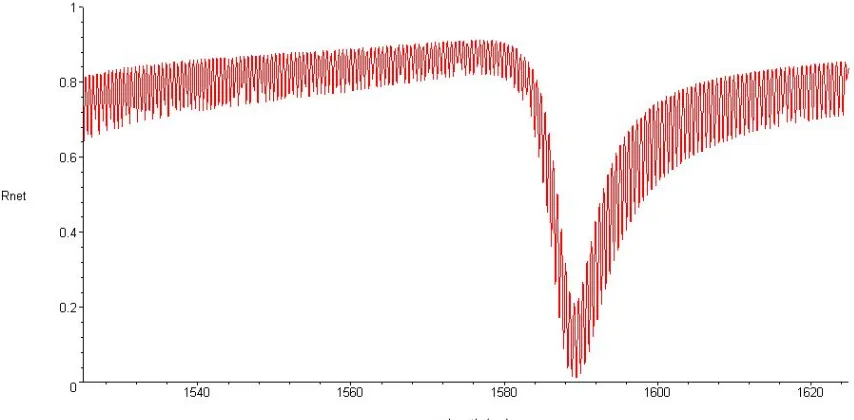
were used to determine the net reflectance of the stack. The plot in Figure 2.8 shows the net

reflectance of the stack using the characteristic matrix analysis.

Figure 2.8 - Plot of net reflectance (using transfer matrix method) of the stack of various materials as a function of the incident wavelength.

From the plot, two sources of interference can be seen. The large dip in the plot is

(40)

used in the experiment. The shorter period interference pattern that modulates on top of the

longer period interference pattern comes from the interference of the thick plate glass

substrate. One way to minimize this unwanted interference is to apply an anti-reflection

coating to the bottom of the plate glass. This will reduce the magnitude of the unwanted

interference and will yield only the desired reflection interference minima caused by the

microcavity. An ideal anti-reflection coating would have index

213 . 1 472 .

1 =

= = nairnglass

n and thickness d =λ₀ /4n= 1575/4(1.213) = 324.6nm. The

reflectance of the same stack as in Figure 2.8 but with an AR coating of index 1.213 and

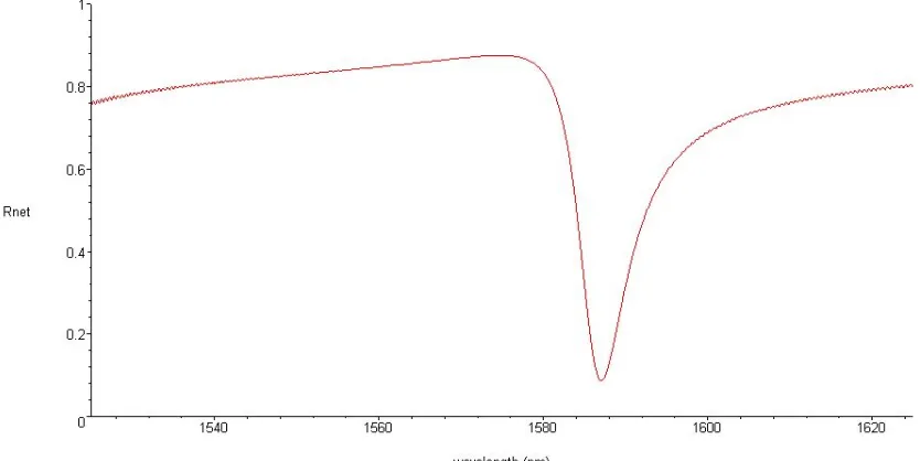
thickness 324nm is shown in the Figure 2.9.

Figure 2.9 - Plot of the net reflectance (using transfer matrix method) of the stack of materials with an ideal AR coating on the bottom of the plate glass to prevent optical interference of the glass layer.

The curve is much smoother because interference from the glass substrate is

minimized. The AR film with index closest to the desired 1.213 is MgF2 with a refractive

(41)

because of its low refractive index. A plot of the net reflectance of the same stack with a

293nm thick AR coating of MgF2 is shown in Figure 2.10.

Figure 2.10 - Plot of the net reflectance (using transfer matrix method) of the stack of materials with a 293nm thick AR coating of MgF2 (n=1.346).

Though the AR coating is not needed, it is preferred in order to get the maximum

amount of light to the cavity. Any bridge motion can still be seen but the signal may not be

as clean and strong as it would if there was an AR coating. Most of these fast oscillations

within the reflectance scans will not be seen due to the size of the laser spot. Even for very

high quality optical flats, most of this interference will get cancelled out over the round trip

within the stack.

When the interrogation laser is tuned to the wavelength of sharpest slope, small

movements of the beam can be detected optically. As the microcavity separation changes,

the intensity of the reflected light will change correspondingly. Any resonant motion of the

(42)

2.9 References

1

M. Xiang, Y. Cai, Y. Wu, J. Yang, Y. Wang, “Fabrication and analysis of Fabry-Perot cavity with a micromechanical wet-etching process,” Applied Optics, volume 43, pp. 3258-3262, Jun. 2004.

2

D. Hohlfeld, M. Epmeier, H. Zappe, “A thermally tunable, silicon-based optical filter,” Sensors and Actuators A, volume 103, pp. 93-99, 2003.

3

J. Correia, M. Bartek, R. Wolffenbuttel, “Bulk-micromachined tunable Fabry-Perot

microinterferometer for the visible spectral range,” Sensors and Actuators A, volume 76, pp. 191-196, 1999.

4

M., Stephens, “A Sensitive Interferometric Accelerometer,” Review of Scientific Instruments, volume 64, pp. 2612-2614, Sep. 1993.

5

C. Zhou, S. Letcher, and A. Shukla, “Fiberoptic Microphone Based On A Combination Of Fabry-Perot Interferometry And Intensity Modulation,” Journal of the Acoustical Society of America, volume 98, pp. 1042-1046, Aug. 1995.

6

J. Huang, K. Liew, C. Wong, S. Rajendran, M. Tan, A. Liu, “Mechanical design and optimization of capacitive micromachined switch,” Sensors and Actuators A, volume 93, pp. 273-285, 2001.

7

Y. Kim and D. Neikirk, “Micromachined Fabry-Perot Cavity Pressure Transducer,” IEEE Photonics Technologies Letters, volume 7, pp. 1471-1473, Dec. 1995.

8

A. Baldi, W. Choi, B. Ziaie, ”A Self-Resonant Frequency-Modulated Micromachined Passive Pressure Transensor,” IEEE Sensors Journal, volume 3, pp. 728-733, Dec. 2003.

9

X. Wang, B. Li, O. Russo, H. Roman, K. Chin, K. Farmer, “Diaphragm design guidelines and an optical pressure sensor based on MEMS technique,” Microelectronics Journal, volume 37, pp. 50-56, 2006.

10

JS Harper, PA Rosher, S Fenning, SR Mallinson, “Application of Miniature

Micromachined Fabry-Perot Interferometer to Optical Fiber WDM System,” Electronics Letters, volume 25, pp. 1065-1066, Aug. 1989.

11

N. Lavrik, M. Sepaniak, P. Datskos, “Cantilever transducers as a platform for chemical and biological sensors,” Review of Scientific Instruments, volume 75, pp. 2229-2253, Jul. 2004.

12

(43)

13

X. Liu, S.F. Morse, J.F. Vignola, D.M. Photiadis, A. Sarkissian, M.H. Marcus, and B.H. Houston, “On the modes and loss mechanisms of a high Q mechanical oscillator,” Applied Physics Letters, volume 78, pp. 1346-1348, Mar. 2001.

14

T. Stievater, W. Rabinovich, H. Newman, J. Ebel, R. Mahon, D. McGee, and P. Goetz, “Microcavit”y Interferometry for MEMS Device Characterization,” J.

Microelectromechanical Systems, volume 12, pp. 109-116, Feb. 2003.

15

T. Stievater, W. Rabinovich, H. Newman, J. Ebel, R. Mahon, D. McGee, and P. Goetz, “Measurement of thermal-mechanical noise in microelectromechanical systems,” Applied Physics Letters, volume 81, pp. 1779-1781, Sep. 2002.

16

J. Verdeyen, Laser Electronics. Englewood Cliffs, N.J.: Prentice Hall, 1994, pp. 123-139.

17

E. Eklund and A. Shkel, “Factors affecting the performance of micromachined sensors based on Fabry-Perot interferometry,” Journal of Micromechanics and Microengineering, volume 15, pp. 1770-1776, Sep. 2005.

18

C. Denker, A. Tritschler, “Measuring and Maintaining the Plate Parallelism of Fabry-Perot Etalons,” Publications of the Astronomical Society of the Pacific, volume 117, pp. 1435-1444, Dec. 2005.

19

D. Jones, J. Bland-Hawthorn, “Parallelism of a Fabry-Perot Cavity at Micron Spacings,” Publications of the Astronomical Society of the Pacific, volume 110, pp. 1059-1066, Sep. 1998.

20

M. Born and E. Wolf, Principles of Optics: Electromagnetic Theory of Propagation, Interference and Diffraction of Light. New York: Cambridge University Press, 1999.

21

D.W. Berreman, "Optics in Stratified and Anisotropic Media: 4X4-Matrix Formulation," Journal of the Optical Society of America, volume 62, pp. 502-510, Apr. 1972.

22

(44)

3 MICROMECHANICAL THEORY

3.1 Introduction

The emerging field of micro-electromechanical systems (MEMS) has rapidly evolved

in recent years. One of the benefits came from years of integrated circuits processing

technologies such as photolithography, thin-film deposition, and chemical/plasma etching1,2.

For the most part, the characterization of MEMS consists of the mechanical properties of

these devices. Following these lines, one of the primary goals of this work is to understand

the mechanics of the micromachined double-clamped beam, the desired device type for the

cavities. This section contains the theory of the motion of the double-clamped beam

including the effect air-damping has on its motion.

It is important to note that the measurements for the resonant frequencies derived in

this analysis will not be taken as the theoretical values for the devices in this work. Much of

the mechanical theory is complicated by the aluminum coating on the bridges. This analysis

will simply be used as a means of getting a first-order idea of the frequencies to be expected.

Also, by using the estimated frequencies, this analysis can be used as a means of determining

the dimensions and scale of the devices to be created.

3.2 Double-Clamped Beam

A double-clamped beam, displayed in Figure 3.1, is a microscale device which is held

on its ends to create a bridge.

(45)

Figure 3.1 - Simple model of a double-clamped beam of width w, thickness t, and length L. The length of the beam is along the x-axis and the width is along the y-axis. Each side of the beam is supported by a spacer of a known height h.

3.3 Euler-Bernoulli Theory

The Euler-Bernoulli theory, a simplified analysis from the theory of elasticity, can

describe the dynamics of a double-clamped beam provided that the beam obeys the following

properties: a) the length is significantly greater than both the width and thickness, b) the

cross-sectional area of the beam is constant along the total length, c) the beam is loaded in its

plane of symmetry, without any torsion, d) any deflections of the beam are small compared

to the length, e) the material used for the beam is isotropic, and f) the plane sections of the

beam remain plane. The motion along the z-direction Y( tx, )as a function of both

longitudinal displacement and time is described by the differential equation3

(46)

whereρ is the density of the beam material, t is the thickness of the beam, w is the width of

the beam, E is Young’s Modulus of Elasticity, I =wt3/12 is the bending moment of

inertia for a double-clamped beam, and q( tx, ) is the external force per unit length on the

beam. The external forces include any driving forces plus any damping terms due to air

resistance. The boundary conditions at x=0 and x=L are given by the equations:

0 ) ( ) 0

( =Y L =

Y _(3.2)

0 ) ( ) 0

( =Y L =

Y& & _(3.3)

where the overdot denotes a time derivative. The solution of the differential equation, which

assumes that there are no external forces, thus q(x,t)=0, is given by the following equation:

t i n n n n n n n n e x k x k C x k x k C t x

Y ( , )=[ ₁ (cos −cosh )+ ₂ (sin −sinh )] −Ω . (3.4)

The eigenvectors k are satisfied by the equation n cosknLcoshknL=1 after applying the

boundary conditions. The first four eigenvectors are given by the following relationships:

L

k_n =4.73004, 7.8532, 10.9956, and 14.1372. The solved values of k can be substituted _n

into the following equation to yield the angular eigenfrequencies:

2 n n k A EI ρ = Ω (3.5)

The eigenfrequencies are given by

2 2 1 2 n n n k A EI ρ π π υ = Ω = (3.6)

Solving for the fundamental frequency yields

2 1

1 1.027

(47)

Table 3.1 – Various material properties used in the resonant frequency analysis

Silicon Nitride Material Property Symbol Value Units

Mass Density ρ 3290 kg/m3

Young’s Modulus of Elasticity E 3.00x1011 N/m2

Beam Thickness t 200 nm

Substituting the silicon nitride material properties into the equation, the fundamental

frequency becomes:

2 3 1 1.961 10

− −

×

= L

υ (3.8)

A plot of equation 3.8 for a silicon nitride beam of various lengths is shown in Figure 3.2.

(48)

The frequencies of the higher order modes are given by υ2 =2.756υ1, υ3 =5.404υ1,

1 4 8.933υ

υ = . Each of these frequencies plus the eigenvectors and constants C1n and C2n are

given in the following table for each of the first four eigenvalues.

Table 3.2 - Various constants associated with the first four transverse modes of a double-clamped beam. 1

=

n n=2 n=3 n=4 L

kn 4.73004 7.8532 10.9956 14.1372

1 /υ

υn 1 2.756 5.404 8.933

L

C₁_n / -1.0000 -1.0000 -0.9988 -1.0000

L

C₂_n/ 0.9825 1.0008 0.9988 1.0000

3.4 Mechanical Quality Factor

A figure of merit describing the motion and more importantly the mechanical energy

dissipation mechanism of the microbeam is the mechanical quality factor. The mechanical

quality factor (Q) is given by the following equation:

dB BW f Q 3 0 − = (3.9)

where f is the resonant frequency and BW is the -3dB bandwidth of the resonance. The ₀

sensitivity of a mechanical oscillator depends on the ratio of the smallest resolvable resonant

frequency shift divided by the resonant frequency. The mechanical Q-factor is important

because it is a way of quantifying the sensitivity; the higher the Q-factor, the lower the

resolvable frequency shift, thus the higher the sensitivity. Because of the dissipation of

energy in a micromechanical resonator, the mechanical Q-factor has a finite magnitude.

Complexities of the motion of the microbeam are due to the length scale dependence of the

resonant frequency and the mechanical quality factor. As the lengths of the beams decrease

(49)

an increase in the air-damping effects, thus decreasing the mechanical quality factor. This

particular double-clamped beam design has two main sources of energy loss: e.c. first is the

intrinsic loss in the beam material which is given by Zener’s model for anelastic solids and

the second and more dominant source of loss is the air damping force exerted on the

resonator. These damping terms must be included in the Euler-Bernoulli theory above, thus

changing the effective resonant frequencies and causing the Q-factor to decrease in value. In

this analysis, only the more dominant air damping force is considered.

3.5 Air Damping Effects

The magnitude of the air damping depends on various physical parameters of the

beam. The type of treatment to be used depends on the separation between the beam and the

underlying substrate. If the separation h, shown in Figure 3.3, is smaller than the width of

the beam, then the type of damping is referred to as squeeze-film damping4,5,6. For any

cavity separations larger than w, an infinite gas medium treatment is more appropriate,

where the drag force shifts from squeeze film damping being the dominant force to the

simple air-damping above and below the beam. The infinite gas limit is based on the Oseen

solution for the drag force on a long cylinder moving in an incompressible fluid7. Here, only

the squeeze-film damping approach is examined since the cavity separation h is smaller than

(50)

Figure 3.3 - Deflected double-clamped beam of thickness t creating a squeezed film a height h above the substrate.

The squeeze film damping effect on a beam resonator, caused by the thin gas layer

between the structure and the supporting substrate, is analyzed on the basis of the coupled

elastic beam theory and the Reynolds equation for isothermal incompressible gas films.

Zhang et al.4,7 described a set of equations using coupled solid deformation and fluid flow

equations which depend only on various beam and fluid properties to solve for the

mechanical Q factor and the effective shift of the resonant frequency. The analysis proceeds

with the pressure distribution of a squeezed-film determined by the Reynolds equation for an

incompressible fluid: t ph y p p h y x p p h x ∂ ∂ = ⎟⎟ ⎠ ⎞ ⎜⎜ ⎝ ⎛ ∂ ∂ ∂ ∂ + ⎟ ⎠ ⎞ ⎜ ⎝ ⎛ ∂ ∂ ∂ ∂ ( ) 12 3 3 μ (3.10)

where p(x,y,z) is the position dependent pressure, μ is the gas dynamic viscosity, and h is

the separation between the beam and the substrate. The boundary conditions are:

a p t w x p t w x

p( , /2, )= ( ,− /2, )=

(51)

where p is the ambient pressure. These boundary conditions assume that the pressure on a

the edges of the beam is equal to the ambient pressure and the pressure at the ends of the

beam remains constant. The fluid properties of air are given in the following table:

Table 3.3 – Fluid properties for air used throughout the squeeze film analysis.

Constant Value Units

Gas Dynamic Viscosity of Air 1.81x10-5 kg·m/s

Ambient Air Pressure 1.013x105 N/m2

Another important term is the squeeze number, σ , given by the equation:

2 0 2 12

h p

L

a

μω

σ = (3.13)

where ω is the excitation frequency of the beam and all other constants are as previously

defined. The squeeze number is a measure of the compressibility of the fluid in the gap. A

plot of the squeeze number σ as a function of the squeeze film thickness h for a beam of ₀