Scholarship at UWindsor
Scholarship at UWindsor
Electronic Theses and Dissertations Theses, Dissertations, and Major Papers
2019
Scalable Methods and Algorithms for Very Large Graphs Based
Scalable Methods and Algorithms for Very Large Graphs Based
on Sampling
on Sampling
Roohollah Etemadi
University of Windsor
Follow this and additional works at: https://scholar.uwindsor.ca/etd
Recommended Citation Recommended Citation
Etemadi, Roohollah, "Scalable Methods and Algorithms for Very Large Graphs Based on Sampling" (2019). Electronic Theses and Dissertations. 7700.
https://scholar.uwindsor.ca/etd/7700
This online database contains the full-text of PhD dissertations and Masters’ theses of University of Windsor students from 1954 forward. These documents are made available for personal study and research purposes only, in accordance with the Canadian Copyright Act and the Creative Commons license—CC BY-NC-ND (Attribution, Non-Commercial, No Derivative Works). Under this license, works must always be attributed to the copyright holder (original author), cannot be used for any commercial purposes, and may not be altered. Any other use would require the permission of the copyright holder. Students may inquire about withdrawing their dissertation and/or thesis from this database. For additional inquiries, please contact the repository administrator via email
Very Large Graphs Based on Sampling
By
Roohollah Etemadi
A Dissertation
Submitted to the Faculty of Graduate Studies through the School of Computer Science in Partial Fulfillment of the Requirements for
the Degree of Doctor of Philosophy at the University of Windsor
Windsor, Ontario, Canada
2019
c
by
Roohollah Etemadi
APPROVED BY:
J. Huang, External Examiner York University
M. Ahmadi
Department of Electrical and Computer Engineering
M. Kargar
School of Computer Science
D. Wu
School of Computer Science
J. Lu, Advisor School of Computer Science
Y. H. Tsin, Co-Advisor School of Computer Science
I. Co-Authorship
I hereby certify that this dissertation incorporates material that is the result of my
research conducted under the supervision of my advisors Prof.s Jianguo Lu and Yung
H. Tsin. In all cases, the key ideas, primary contributions, experimental designs, data
analysis, interpretation, and writing were performed by the author.
I am aware of the University of Windsor Senate Policy on Authorship and I certify
that I have properly acknowledged the contribution of other researchers to my thesis,
and have obtained written permission from each of the co-author(s) to include the
above material(s) in my thesis.
I certify that, with the above qualification, this thesis, and the research to which
it refers, is the product of my own work.
II. Previous Publications
This dissertation includes the extended or original varsion of the papers that have
been previously published/submitted for publication in peer reviewed conferences and
journals, as follows:
• Roohollah Etemadi, Jianguo Lu, and Yung H. Tsin. 2016. Efficient Estimation of Triangles in Very Large Graphs. In Proceedings of the 25th ACM Interna-tional on Conference on Information and Knowledge Management (CIKM ’16). ACM. New York. NY. USA. pp. 1251-1260. doi:10.1145/2983323.2983849. The data and code are publicly available athttp://etemadir.myweb.cs.uwindsor.
ca/cikm2016/triangles.php(Chapter 2).
• Roohollah Etemadi, Jianguo Lu. 2017. Bias Correction in Clustering
Co-efficient Estimation, In Proceedings of the 2017 IEEE International
Confer-ence on Big Data (IEEE BigData’17). Boston. USA. pp. 606-615. doi:
10.1109/BigData.2017.8257976. The code and data are available online at
http://etemadir.myweb.cs.uwindsor.ca/cbias(Chapter 4).
myweb.cs.uwindsor.ca/cbiasstream (Chapter 4).
• Roohollah Etemadi, Jianguo Lu. 2019. PES: Priority Edge Sampling in Stream-ing Triangle Estimation, IEEE Transactions on Big Data (TBD), 2019 (Under revision). The code and data are available online athttp://etemadir.myweb.
cs.uwindsor.ca/PES (Chapter 3).
• Roohollah Etemadi, Jianguo Lu. 2019. Bias Correction in Streaming and Non-streaming Algorithms in Clustering Coefficient Estimation, IEEE Transactions on Knowledge and Data Engineering(TKDE), 2019 (Under review). The code
and data are available online athttp://etemadir.myweb.cs.uwindsor.ca/cc
(Chapter 4).
I certify that I have obtained a written permission from the copyright owner(s)
to include the above published material(s) in my thesis. I certify that the above
material describes work completed during my registration as a graduate student at
the University of Windsor.
III. General
I declare that, to the best of my knowledge, my thesis does not infringe upon
any-ones copyright nor violate any proprietary rights and that any ideas, techniques,
quotations, or any other material from the work of other people included in my
the-sis, published or otherwise, are fully acknowledged in accordance with the standard
referencing practices. Furthermore, to the extent that I have included copyrighted
material that surpasses the bounds of fair dealing within the meaning of the Canada
Copyright Act, I certify that I have obtained a written permission from the copyright
owner(s) to include such material(s) in my thesis. I declare that this is a true copy
of my thesis, including any final revisions, as approved by my thesis committee and
the Graduate Studies office, and that this thesis has not been submitted for a higher
size of networks. Direct analysis is even impossible when the network data is not entirely accessible. For instance, user networks in Twitter and Facebook are not available for third parties to explore their properties directly. Thus, sampling-based algorithms are indispensable.
This dissertation addresses the confidence interval (CI) and bias problems in real-world network analysis. It uses estimations of the number of triangles (hereafter ∆) and clustering coefficient (hereafter C) as a case study. Metric ∆ in a graph is an important measurement for understanding the graph. It is also directly related to C
in a graph, which is one of the most important indicators for social networks. The methods proposed in this dissertation can be utilized in other sampling problems.
To my parents and siblings with gratitude.
To my dear and loving wife with love.
I would like to express my sincere gratitude to my advisors, Professor Jianguo
Lu and Professor Yung H. Tsin, for their continuous support of my Ph.D. study and
research, for their extensive professional guidance, and for their immense knowledge.
I am greatly indebted to my dissertation committee, Professor Jimmy Huang,
Professor Majid Ahmadi, Doctor Dan Wu, and Doctor Mehdi Kargar for participating
in my seminars, for taking time to read my dissertation, and for providing me with
their valuable comments.
I would also like to thank the Ontario Government, and the committee of Faculty
of Graduate Studies of the University of Windsor for awarding an Ontario Graduate
Scholarship (OGS) to me.
In addition, my thanks goes to NSERC (Natural Sciences and Engineering
Re-search Council of Canada) and School of Computer Science for supporting my reRe-search
through my advisors’ grants, and for offering me GAships and TAships respectively.
I owe special thanks to the staff of School of Computer Science, Ms. Karen
Bourdeau, Ms. Christine Weisener, Ms. Melissa Robinet, Ms. Gloria Mensah, Mr.
Maunzer Batal, and Mr. Robert Mavrinac for their great support.
I would like to acknowledge Canterbury College and its outstanding staff’s
con-tribution in providing a comfortable and friendly student residence, where I always
felt supported and welcome.
It is my privilege to thank my wife, Dr. Sholaeh Hashemi Namin, for her unending
inspiration and support throughout my studies.
Last but not least, I am thankful to my parents, my parents-in-law, and my
DECLARATION OF CO-AUTHORSHIP/PREVIOUS PUBLICATION III
ABSTRACT V
DEDICATION VI
ACKNOWLEDGEMENTS VII
LIST OF TABLES XI
LIST OF FIGURES XII
1 Introduction 1
1.1 Introduction . . . 1
1.2 Challenges in network graphs analytics . . . 1
1.3 Framework of sampling methods . . . 3
1.3.1 Take samples . . . 3
1.3.2 Generalization . . . 4
1.3.3 Variance vs sample size . . . 6
1.4 Motivation . . . 7
1.5 Review of our contributions . . . 10
1.6 The structure of the dissertation . . . 13
2 Estimation of Triangles 14 2.1 Introduction . . . 14
2.2 Related work . . . 16
2.3 Methods . . . 17
2.3.1 Motivation . . . 17
2.3.2 Our method . . . 19
2.3.3 Variance of EG . . . 21
2.3.4 Variance of Eg . . . 23
2.4 Experiments . . . 26
2.4.1 Datasets . . . 26
2.4.2 Experimental setup . . . 26
2.4.3 Verification of Theorems . . . 30
2.5 Discussions and conclusions . . . 32
3 PES: Priority Edge Sampling in Streaming Triangle Estimation 35 3.1 Introduction . . . 35
3.2 Background and related work . . . 36
3.2.1 Node-based methods . . . 37
3.2.2 Edge-based methods . . . 38
3.4.2 Example . . . 43
3.4.3 The unbiased estimator . . . 45
3.4.4 The variance . . . 47
3.5 Experiments . . . 49
3.5.1 Data . . . 50
3.5.2 Comparison with GPS-In and GPS-Post . . . 50
3.5.3 Validation of Theorems 1 & 3 . . . 55
3.5.4 An implication of Theorems 1 & 3 . . . 56
3.6 Conclusions and discussions . . . 57
4 The Bias and Variance in Clustering Coefficient Estimation 59 4.1 Introduction . . . 59
4.2 Background and related work . . . 62
4.2.1 Related work . . . 63
4.3 The bias and variance in a non-streaming model . . . 66
4.3.1 The sampling scheme . . . 66
4.3.2 The bias . . . 67
4.3.3 Counting Ψ and Ω . . . 70
4.3.4 The variance . . . 72
4.4 The bias and variance in a streaming model . . . 74
4.4.1 Naive edge streaming (NES) . . . 74
4.4.2 Estimator of the variance . . . 76
4.4.3 The bias-corrected estimator . . . 78
4.4.4 The variances of ∆g and Λg and their covariance . . . 79
4.5 Experiments . . . 81
4.5.1 Datasets . . . 81
4.5.2 The bias in the non-streaming model . . . 81
4.5.3 Positive and negative bias . . . 84
4.5.4 Characterizing bias using second and third moments . . . 85
4.5.5 When the bias is large . . . 87
4.5.6 Verification of Theorem 2 . . . 87
4.5.7 Verification of Theorem 3 . . . 87
4.5.8 The bias in the streaming model . . . 92
4.6 Discussions and conclusions . . . 93
5 Conclusions and Future Directions 95 5.1 Introduction . . . 95
5.2 Discussions and conclusions . . . 95
5.3 Impact of our dissertation research . . . 97
5.4 Looking into the future . . . 97
2.1 Summary of the notations. . . 18
2.2 Properties of the networks in our experiments, sorted by graph sizeN. 25
3.1 Summary of the notations . . . 37
3.2 Properties of the networks in our experiments, sorted by graph sizeN. 49
4.1 Summary of the notations . . . 63
1.1 The framework of sampling approaches for network analytics. . . 3
1.2 Examples of sampling methods. . . 4
1.3 Examples of unbiased and biased estimators. EstimatorXb is repeated
k times and the estimation of metric X in run i = 1,2, .., k is shown
byXbi, and the expectation isE[Xb] = k1 Pk
i=1Xbi. . . 6
1.4 Examples of estimations with small (Panel A) and large (Panel B)
variances. . . 6
1.5 The Confidence Interval problem of existing methods to estimate ∆.
The properties of the input graph need to be used to construct the
confidence interval using (, σ)-approximation and the variance. . . . 7
1.6 The bias problem of existing methods to estimate C. . . 8
1.7 Overview of our contributions to estimate ∆. The estimator of variance
used to construct confidence interval. . . 10
1.8 Overview of our contributions to estimate C. The bias quantified and
the bias-corrected estimators proposed for the first time. . . 11
2.1 Illustration of Eg and EG sampling. . . 20
2.2 Dependent wedges of two shared triangles. . . 21
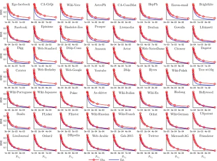
2.3 The observed and estimated RSEs of estimator EG. Estimated values
are obtained from Eq. 10. . . 28
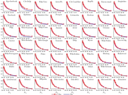
2.4 The observed and estimated RSEs of estimator Eg. Estimated values
are based on Eq. 11. . . 29
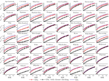
2.5 The observed and estimated ratio between the sample sizes of
esti-mators Eg and EG with the same RSE. Estimated value are obtained
based on Eq. 13. . . 31
2.6 Improvement as a function of data size M and ∆. RSE=0.1. . . 33
B), and NES (Panel C) when RSE=0.2. . . 51
3.3 Our PES usesless sample sizescompared to other methods to obtain
an estimation with the same RSE=0.2 on most of the graphs. Note
that the sample size include both the size of the subgraph and the
reservoir for our PES but for GPS methods extra memory per sampled
edge was ignored. . . 52
3.4 Our PES outperforms GPS-In in terms of RSEs when both methods
are using the same sample sizes. Note that for our PES, the sample
size includes both the size of subgraph g and reservoir size, i.e., |σ|.
For GPS-In, we only considered the size of subgraphg as a sample size,
and ignored two additional values per sampled edge ing. . . 53
3.5 The observed RSEs of∆P ESb support our estimated RSEs based on Eq.
14. . . 54
3.6 The observed RSEs of ∆N ESb fit very well our estimated RSEs based
on Eq. 3. . . 55
3.7 Our PES outperforms NES. The observed and estimated ratios between
pN and pD when the methods achieve the same RSEs between 0.1 and
0.4. The estimated ratios are obtained using Eq. 16. . . 57
4.1 Illustration of shared wedges and closed-wedges. (a) A sample graph;
(b) Wedge (l, j, i) shares with wedge (k, j, i); (c-d) Wedge (l, j, i) shares
with closed-wedges (i, j, k), (k, i, j); (e) Wedge (l, j, k) shares with
closed-wedge (j, k, i). The large node in the plot indicates the
cen-tre node of the closed-wedge. E.g., in Panel (c) the closed-wedge is
(k, j, i). . . 68
4.2 An example for computing Ψ and Ω in the sample graph in Fig. 4.1
5×10⁴ independent runs for all graphs except for the large graphs in
the last row with 104 independent repetitions. The estimated RBs are
obtained using Eq. 17. . . 83
4.4 The bias-corrected estimator Cb+ vs. biased estimator. The observed
RBs were obtained over 5×10⁴ independent runs for all graphs except
for the large graphs in the last row with 104 independent repetitions. 84
4.5 RB depends on the first term and second term of the Taylor expansion.
The outliers are the 10 smallest graphs. Observed RBs are taken when
RSE=0.2 over 105 independent runs. . . . 88
4.6 ΛΨ2 against
2hd3i
Nhd2i2 for 56 graphs. . . 89
4.7 A sample of the Stanford Web network. . . 89
4.8 The observed vs. the estimated RSEs. Estimated RSEs are obtained
based on Eq. 32 over 100 independent runs. . . 90
4.9 The observed RSEs ofCbfit perfectly the estimated RSEs based on Eq.
39 in representative graphs. . . 91
4.10 The estimated RSEs obtained based on Eq. 40 are apt estimations for
the observed RSEs of Cb. . . 91
4.11 The observed RBs of Cb(biased estimator) support our estimations of
RB based on Eq. 47. . . 92
4.12 Our biased-corrected Cb+ removes the bias perfectly. . . 92
4.13 Comparison of sample sizes, i.e. number of sampled edges, of the
methods when RSE=0.2. The sample size of NES is comparable with
Introduction
1.1
Introduction
Most of the data in real-world are in the form of networks. Online social networks
such as Facebook, Twitter, and many more are examples of such network data. In
academia, co-authorship and citation networks are other examples. Such network
data are modeled by graphs. Analyzing such network graphs attracts increasing
attention from industry and academia in recent years. However, the nature of such
network graphs bring some challenges. This chapter outlines the main challenges in
analyzing real-life network graphs. It also reviews possible solutions in this direction.
Then, the main contributions of this dissertation will be outlined. The final section
will contain the structure of the rest of this dissertation.
1.2
Challenges in network graphs analytics
Many metrics such as network size, average degree, average shortest path length,
graph centralities such as PageRank, betweenness, Katz, the number of triangles, and
clustering coefficient have been utilized to analyze the complex structure of network
graphs. Moreover, a number of tools and APIs such as NoSQL, NetworkX, and
GraphX have been developed to compute such metrics in recent years. However,
computing exact values of graph metrics are computationally an intensive task or
even impossible in the following scenarios.
• Big data: When the size of the graph is large or even medium, exact
com-puting of most of the graph metrics is infeasible or even impossible due to the
massive in their size. For example, Facebook had more than 2 billion monthly
active users as the second quarter of 2018 1. Another example is the Internet
with more than 5.48 billion web pages over the world by March 20192. Neuronal
networks, Protein-protein and DNA–protein interaction networks are other
ex-amples from the biology domain. Such network data result in constructing
graphs with millions of nodes and billions of edges. Thus, applying exact
algo-rithms on massive network graphs is computationally demanding. For example,
enumerating triangles using the best-known algorithm has a time complexity of
O(M3/2) [2, 3], where M is the number of edges in the input graph. Obviously,
applying such a method for example on Facebook network graph with billion of
edges is inefficient.
• Hidden data: The entire data are inaccessible for third parties in most of the
real networks. For example, the network data of online social networks such
as Facebook and Twitter are hidden behind search-able interfaces due to the
privacy of their users. Hence, exact computing is impossible when the data are
not entirely available.
Thus, designing efficient methods to deal with such challenges are indispensable.
One possible solution is to utilize high-speed machines, and parallel and distributed
computations. However, such a solution is costly and not available for all.
Further-more, the exact computing is not essential in many real applications. Therefore, the
accuracy can be traded against computation time and memory usage. Thus, an
es-timation with confidence interval using reasonable time and memory is desired. In
such a case, sampling techniques have largely been utilized to estimate network graph
statistics [4–13]. Sampling methods take a small amount of data from a massive
net-work graph. Then, the properties of the sampled data are generalized to the entire
network. Obviously, the sampled data is much smaller than the original one. Thus,
analyzing sample data needs less CPU time and memory usage. Furthermore, the
entire data are not required in case of hidden data.
1https://www.statista.com
1. Take Samples
3. Generalization 2. Study subgraph g
Subgraph g
Original graph G
Unknown metrics
X =N, M,∆, ... Xg : X ing
e.g. ∆g: 7 triangles in g
b
X : estimator for X
E(Xb) =?, |Xb−X|=? e.g. ∆ = 1b ,623,244, |∆b −∆|=?
FIGURE 1.1: The framework of sampling approaches for network analytics.
1.3
Framework of sampling methods
Suppose network data are modeled by graphGand metrics ofGsuch as the network
size N, the number of edges M, average degree hdi, degree distribution, the number
of triangles ∆, clustering coefficientC, average shortest path length, etc are unknown.
The goal is to design a sampling method to take subgraph g from original graph G
and study the metrics of G using statistics of sampled graph g. The framework of
such a sampling technique is shown in Fig. 1.1. It takes samples from the original
graphGto create subgraphg and generalizes the properties ofg to the original graph.
In other words, it aims to design estimatorXb for metric X inG. The following steps
need to be considered to design estimator Xb.
1.3.1
Take samples
The first step is to take sample data to create subgraphg. Different sampling methods
can be used to sample data. Such methods depend on the way to access to the original
graph G. Methods can have random or sequential access to the whole or part of the
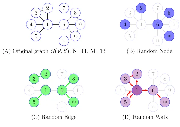
1 2 3
4
5
6 7
8
9
10 11
1
2
3
4
5
6
7
8
9
10 11
(A) Original graphG(V,E), N=11, M=13 (B) Random Node
1 2 3
4
5
6
7
8
9
10 11
1 2 3
4
5
6
7 8
9
10 11
1
(C) Random Edge (D) Random Walk
FIGURE 1.2: Examples of sampling methods.
Fig. 1.2 shows three graph sampling methods on a toy graph in Panel A. When
random access to graph G is available, Random Node (Panel B) or Random Edge
(Panel C) methods can be used to take samples. For example, 5 random nodes are
selected in Panel B. Random Walk (Panel D) is an option when the network data
is not entirely available. It starts from a node (node 1 in Panel D) at random and
explores the graph by randomly walking on the edges. Note that different sampling
schemes need to be designed to estimate different metrics. In other words, designing
a sampling method depends on the metric of interest.
Graph sampling approaches are categorized based on their access to the original
graph into two main models: streaming and none-streaming. In the former model, a
limited number of sequential passes over the stream of graph data are used to take
samples. In the later model, random access to the original graph data is available.
The goal of methods in both models is to obtain an accurate estimation using a
limited memory window to store sampled data.
1.3.2
Generalization
After taking sampled data, the next step is generalizing the properties of sampled
sampled data to the original network. Two important tasks need to be done in this
step.
• Unbiasedness vs biasness: The first task is to show that the estimation is
biased or unbiased. The desired estimator is unbiased, i.e. the expectation of
the estimations of a metric needs to be the same as the true value of the metric.
Let Xb be an estimator for metric X. Estimator Xb is unbiased if E[Xb] = X;
otherwise it is biased. For a biased estimator, the bias needs to be quantified
and corrected. Examples of unbiased and biased estimators are shown in Fig.
1.3. Suppose estimator Xb is repeated k times and Xbi is the estimation in
repetition i. Panel (A) shows an unbiased estimator. When k is large enough,
E[Xb] = 1k Pk
i=1Xbi = X. In contrast, the estimator Xb in Panel (B) is biased because the expectation of the estimations (E[Xb]) is far away from the true value
of metricX. Thus, for each estimator, one needs to prove the unbiasedness and
for biased estimators, the bias needs to be quantified and corrected.
• Confidence interval: The other important task is to construct the confidence
interval (hereafter CI) of the estimator. In other words, one needs to show that
the estimation is how far away from the true value with a specific confidence.
Suppose, for example, the number of complete subgraphs with size three
(trian-gles) in graphG needs to be estimated. As shown in Fig. 1.1, the estimation of
∆ inGis 1,623,244 using the number of triangles ing(∆g = 7). The question is
that how accurate is∆ = 1b ,623,244 or|∆b−∆|=?. To answer such a question,
one needs to construct the CI of the estimator. Thus, constructing the CI to
understand the error bound of an estimator with a certain confidence level is
an indispensable task.
Several methods have been used to form the CI. When the variance of an
es-timator is not available, Hoeffding’s inequality can be used [14]. Chebyshev’s
inequality is another option to have more accurate bound using the variance
of the estimator [15]. However, using such methods has several drawbacks on
(A) unbiasness (B) biasness
E[Xb] =X E[Xb]6=X
FIGURE 1.3: Examples of unbiased and biased estimators. EstimatorXb is repeated
k times and the estimation of metric X in run i= 1,2, .., k is shown by Xbi, and the expectation is E[Xb] = k1
Pk i=1Xbi.
(A) (B)
FIGURE 1.4: Examples of estimations with small (Panel A) and large (Panel B) variances.
the resulting bounds are not tight enough. More importantly, the properties of
the original graphGshould be known in advance to use such inequalities. Note
that the properties of G are unknown in sampling scenario. Thus, we argue
that using (, δ)-approximation is not practically useful to control the accuracy
of estimators on massive networks. In practice, the properties of sampled graph
g need to be used to construct the CI.
1.3.3
Variance vs sample size
The main goal of sampling algorithms is to achieve an estimation with a small error
bound (variance) by using a small number of samples. Let n be the sample size of
estimator Xb. The relation between the variance of Xb and its sample sizen is:
var(Xb)∝ 1
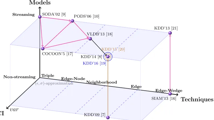
CI
Techniques Models
Triple
Edge-Node
Neighborhood
Edge
Edge-Wedge Streaming
Non-streaming
(, σ)-approximation
var
KDD’09 [7]
SIAM’13 [16] SODA’02 [9]
COCOON’5 [17]
PODS’06 [10]
VLDB’13 [18]
KDD’16 [19]
KDD’15 [20] KDD’14 [8]
KDD’13 [21]
FIGURE 1.5: The Confidence Interval problem of existing methods to estimate ∆. The properties of the input graph need to be used to construct the confidence interval using (, σ)-approximation and the variance.
According to Eq. 1, the variance of an estimator is inversely correlated with its
sample size, i.e. the variance increases by decreasingn. Thus, designing an estimator
to obtain accurate estimations (low variance) using small sample sizes is challenging.
The desired estimator needs to use a small number of samples to obtain estimations
with small variance. For example, suppose both the estimators in Panels (A) and (B)
in Fig. 1.4 use the same sample sizes to estimate X. The estimator in Panel (A) is
preferable due to the small variation of estimations.
1.4
Motivation
A number of sampling-based approaches have been proposed to estimate graph
met-rics such as network size, e.g. in [11, 12, 22–24], average shortest path length [25, 26],
the number of triangles ∆, e.g. in [1, 7–10, 19–21, 27, 28], clustering coefficient C
[1, 8, 29, 30], and many more. We visualized sampling methods to estimate ∆ in Fig.
1.5 andC in Fig. 1.6 in recent years. We make several observations as follows:
• Existing methods use properties of original network graphs to construct CI.
Bias
Techniques Models
Wedge
Neighorhood
Edge-wedge
Edge
Priority Streaming
Non-streaming
Unbiased
Biased
JGAA05 [6], SDM13 [31] VLDB’13 [18]
TKDD15 [29]
KDD’13 [21]
KDD’14 [8]
VLDB’17 [1]
TWEB15 [32]
WWW’13 [23]
FIGURE 1.6: The bias problem of existing methods to estimate C.
confidence interval. Later, the variance has been used by methods to obtain
tighter error bounds. However, both (, σ)-approximation and variance
tech-niques require the properties of the original network to construct the CI. Thus,
such techniques are not useful when the properties of the original network are
unknown which is the case in sampling scenarios.
• The random edge based methods are efficient to estimate metric C; but they
suffer from the bias problem as shown in Fig. 1.6. The bias problem was noticed
in the literature [1, 8, 29]. However, to the best of our knowledge, the bias was
not quantified and not corrected. Thus, it is left as an open problem.
• The estimation of ∆ and C is an active and hot topic in top-tier conferences
and journals. Thus, designing efficient estimators for the properties of real-life
networks is indispensable.
Motivated by those observations, this dissertation addresses the CI and bias
prob-lems in graph sampling methods. It uses two case studies, i.e. the estimation of the
number of triangles and its close metric, clustering coefficient, to study such
prob-lems. However, our techniques to construct CI and to quantify the bias can be used
Metrics ∆ and C are important to reveal the complex structure of real-world
networks specially online social networks. They have been used in many applications
such as community detection [33], graph clustering [34], link prediction [35], spam
detection [36], finding interesting individuals [37] , characterizing the structure of
balanced network [38], wireless and ad hoc networks analysis [39], blog analysis in
online social networks, DAN sequence analysis [40], prediction of essential proteins
[41], microarray data analysis for finding cancer genes [42, 43], identifying modular
formations in protein-protein interaction network [44], risk analysis in economy [45],
word-learning in education [46], and many others.
Based on the nature of real-life networks, different scenarios have been considered
to study the estimation of metrics ∆ andC [7, 10, 23]. In this dissertation, we assume
that the network data is modeled as an undirected and simple graph. Hereafter we
will use terms original and input graph interchangeably to call the input network
graph. Suppose G is an undirected and simple network graph. We will address the
following problems in the rest of this dissertation.
Firstly the estimation of ∆ andC will be discussed in a non-streaming model which
the random access to the original graph is provided. Thus, we define the problem as
follows:
Problem 1. Suppose that edges/nodes of original graph G are accessible uniformly
at random. Design a sampling method to estimate ∆ and C in graph G. What is the
best sampling method to estimate ∆ and C? How the sampled data can be used to
estimate the error bound of the estimation?
Next, we study the estimation of the metrics in a streaming model. The sequential
access to the network data is provided in this model instead of uniform random access.
The goal is to achieve an accurate estimation by storing a small fraction of data
using a single pass or a limited number of passes over the network data. Thus, our
second focus will be as follows.
Problem 2. Suppose that edges of graph G come in an arbitrary (random) order
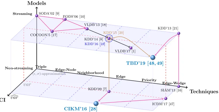
CI
Techniques Models
Triple
Edge-Node
Neighborhood
Edge
Priority
Edge-Wedge Streaming
Non-streaming
(, σ)-approximation
var
d
var
KDD’09 [7] SIAM’13 [16]
CIKM’16 [28]
ICDM’17 [47] SODA’02 [9]
COCOON’5 [17]
PODS’06 [10]
VLDB’13 [18]
KDD’16 [19]
KDD’15 [20] KDD’14 [8]
KDD’13 [21]
VLDB’17 [1]
TBD’19 [48, 49]
FIGURE 1.7: Overview of our contributions to estimate ∆. The estimator of variance used to construct confidence interval.
memory window to store the sampled data over a single pass on the stream.
1.5
Review of our contributions
This dissertation addressed the CI, and the bias problems in sampling methods to
analyze large-scale networks. The main contributions of this dissertation are
summa-rized as follows.
• To estimate ∆: We proposed two new methods to estimate the number of
triangles based on random edge sampling in both streaming and non-streaming
models (see Fig. 1.7). Our methods improve the traditional random edge
sam-pling by probing the edges that have a higher probability of forming triangles.
The methods outperform the existing methods consistently and can be
bet-ter by orders of magnitude when the graph is very large. The results were
demonstrated on 56 graphs, including the largest graphs we can find. More
importantly, we proved the improvement ratio and verified our result on all the
datasets. The analytical results were achieved by simplifying the variances of
Bias
Techniques Models
Wedge
Neighorhood
Edge-wedge
Edge
Priority Streaming
Non-streaming
Unbiased
Biased
Bias-corrected
JGAA05 [6], SDM13 [31] VLDB’13 [18]
TKDD15 [29]
KDD’13 [21]
KDD’14 [8]
VLDB’17 [1]
IEEEBigData’17 [30] TKDE’19 [50, 51]
TWEB15 [32]
WWW’13 [23]
FIGURE 1.8: Overview of our contributions to estimate C. The bias quantified and the bias-corrected estimators proposed for the first time.
that such big data assumption can lead to interesting results not only in triangle
estimation but also in other sampling problems.
• To estimateC: Biased-corrected estimators in the streaming and non-streaming
models were proposed (see Fig. 1.8). Although edge-sampling based methods
are efficient, they result in a biased estimator for C noticed in the literature,
e.g. in [1, 8, 21, 29]. However, the bias has not been quantified and not
cor-rected. Thus, we used quadratic Taylor expansion to quantify the bias of the
estimators. We found that the bias hangs on the structure of input graphs. To
the best of our knowledge, we are the first one who could quantify the bias of
such estimators. To sum up, our contributions in this direction are proposing
the estimators of the bias and the variance of the estimators for C. The bias
and variance phenomenon varies greatly from a graph to graph. To find out the
patterns behind, we conducted extensive experiments with many different kinds
of graphs. In total, we utilized 56 real-life graphs from a variety of areas such as
online social networks, web graphs, Co-authorship, and citation networks. The
graph size also varies from about 4×10³ (very small) to 65×106 (very large).
The experiments reveal that the bias ranges widely from data to data. The
streaming model or can be negative. For most of the graphs, the bias is small,
although every graph does have a bias as quantified by our analytical results.
• Analytical results: We derived the theoretical results of the proposed
esti-mators. Moreover, we quantified the performance ratio between the methods
for the first time. We demonstrated that our results are data independent, i.e.
proposed methods can be run on any real-world network graph without any
restriction on the structure of the graph.
• Big data assumption: The analytical results of the estimators were simplified
to have better insight into them by assuming that the input graph is very large.
Furthermore, we derived the estimators for the variances of the estimators. Our
estimator for the variance has two main implications. First, it can be used to
quantify the performance ratio between the estimators not only for ∆ and C
but also for other metrics. Studying the literature shows that existing methods
were compared using experimental results [1, 8, 10, 18, 19, 21, 29]. The drawback
of such a comparison is that the results are data dependent and vary from data
to data. Thus, we were motivated to give an idea to quantify the performance
ratio between the estimators. Second, it can be used to control the accuracy
of the estimators in practice which is important for practitioners. To use an
estimator in real applications, one needs to decide about the sample size to
achieve an estimation in a given confidence interval. Our simplified estimators
for the variance can be used to determine the sample size of estimators to obtain
an estimation with a given error bound.
• Publicly available data and code: Obtaining ground truth and cleaning
data for a sampling purpose for large graphs are time-consuming tasks. Two
servers with 256GB memory and 24 cores each were used to complete such tasks.
To accelerate the research in this direction, we made the data and our codes
1.6
The structure of the dissertation
The rest of this dissertation is organized as follows. Chapter 2 presents our estimator
for ∆ in a non-streaming model. It contains our analytical and experimental results
for proposed and existing estimators. Our estimator for ∆ in a streaming model will
be discussed in Chapter 3. Furthermore, it presents the derivation of the analytical
results along with their validations using extensive experiments. Our bias-corrected
estimators forC are presented in Chapter 4. The conclusions of the dissertation along
Estimation of Triangles
2.1
Introduction
Graphs are used to model interactions in many applications in online social
net-works, biology, biochemistry, and many other domains. The counts of triangles in
such graphs is an important structural property. For example, in online social
net-works, it is used to measure with what probability friends of friends are also friends
(clustering coefficient [52, 53]). Counting triangles has also various applications such
as spam detection [36] in computer networks, community detection and blog
analy-sis [33] in social networks, protein identification [54], DNA sequence analyanaly-sis [40] in
biology, study of systemic risk [45], tracking the evolution of international trade [55]
in economy, and more.
Enumerating triangles in massive graphs is not practical because the best-known
algorithm has a complexity of O(M1.41) in time and Θ(N2) in space using the fastest
matrix multiplication [3, 56], where N and M are the number of nodes and edges
in the input graph. Thus, sampling algorithms are indispensable. Substantial work
has been done on the streaming model where data items arrive sequentially and
there is a limited memory window [1, 8, 10, 17–20, 29, 57]. Many streaming algorithms
are designed specially to tackle such sampling restrictions. This research focuses
on a more generic sampling scenario without the streaming restriction. It can be
potentially applied to the estimation of triangles in very large graphs, especially when
a graph in its entirety is not available. For instance, many large networks, such as
Twitter and Facebook user network, are hidden behind searchable interfaces. Their
properties can be only estimated by taking a sample from them.
When estimating the number of triangles, the most natural, and a naive one,
is to take triplets (three nodes) uniformly at random, then check whether they form
triangles [9]. Obviously, this method is too costly to be of practical use. Most graphs,
especially the large ones, are sparse. Hence, the vast majority of the triplets have
zero to two edges. It means that the cost of observing even one triangle in this
method will be exorbitantly high. Buriol et al. ameliorate this problem by skipping
the cases for zero edges [10] called EN in this dissertation. They proposed to start
with one random edge, then check whether there are triangles surrounding this edge.
This method can be interpreted as starting with three random nodes, with the
pre-condition that there needs to be at least one edge already in the triplet. When a
random edge is given, there are numerous variations to check whether there is a
containing triangle. [10] takes a random node from the remaining set; [7] continues to
select more random edges hoping to obtain a triangle. The method proposed in [7]
can be regarded as a random edge method: it selects random edges, forms a subgraph
from the random edges. Then the count of the triangles in the subgraph is used to
estimate the number of triangles in the original graph.
Both methods in [10] and [7] still suffer from the scarcity of triangles in the
subgraph. In [10], although it skips the triplets with zero edges, it could be better
also to skip triplets with one edge only, by starting with the triplets that have at least
two edges. For [7], triangle count in the subgraph can increase if we check their edges
not only in the subgraph, but also in the original graph.
Motivated by these observations, we present a new sampling method that combines
the ideas from both [7] and [10]. The first step is the random edge sampling that is
the same as in [7]. Then, for every path of length two in the subgraph, we check the
existence of the third edge in the original graph.
In this dissertation, we give the unbiased estimator and its variance for our
sam-pling method. The variance is a long formula that involves several parameters, thereby
sampling methods. Hence, we simplify the formula based on the assumption that the
graph is very large. The simplified RSE (relative standard error) is 1/p3∆|g, where
∆|g is the number of triangles restricted to the subgraph g. Intuitively, from the
formula we can infer the 95% confidence interval by looking at the triangles in the
subgraph. After doing a similar treatment for the random edge method, we can
com-pare the performance of these two estimators analytically. The analytical analysis
demonstrates that our method is always better than the other method. This is
con-firmed by empirical experiments on 56 graphs, including the largest networks we can
find.
Our contribution is twofold, in both the result and the method. For the result,
we present a new estimator that outperforms the random edge method by orders of
magnitude; For the method, we use the big data assumption to simplify the variances
of various estimators. Thereby, performances of different triangle estimators can be
compared analytically for the first time.
In presenting our theorems, we do not use the −δ approximation notation as
most other papers do, as it is self-evident from Chebyshev’s inequality. What is more,
Chebyshev’s inequality is valid for any data distribution, hence it gives a loose range
that has little practical implication. Estimates produced by multiple runs follow a
normal distribution. This is implied by the central limit theorem and is verified
by our experiments. The central limit theorem can be applied in this case because
each estimation involves the summation (mean) of probabilities for all the triangles
being sampled. With such normal distribution, we have a much tighter confidence
interval, i.e., 95% confidence interval is within two standard deviations. Hence, in
the remaining part of the chapter only RSE and variance are discussed.
2.2
Related work
A number of methods have been proposed to estimate ∆ in streaming and
non-streaming models [1, 7–10,16–21, 29, 47,58, 59]. In a non-streaming model, methods have a
over the network data. In the later model, uniform random access to the network
data is required and the methods do not need to access the whole data. Thus, the
later model is more general and useful when the whole data are not available and this
is the case for real-life networks. Thus, in this chapter, we review methods in a
non-streaming model. We also adjusted methods in a non-streaming model to a non-non-streaming
when it is possible.
A naive method to estimate ∆ istriple sampling[9]. It selects three random nodes
to form a triplet and checks the existence of edges among the nodes. Suppose n is
the number of sampled triplets and v is identified triangles among them. Thus, an
unbiased estimator for ∆ is v N3/n and its variance is ∆ N3−∆2
/n. Obviously,
this method suffers from the paucity of triangles in the sample in sparse graphs which
is the case for real-life networks. Thus, it has been improved by decreasing the sample
space from (N3) toM(N −2) in [10] and called Edge and Node (EN) sampling here.
The idea is to construct a sampled triplet using two connected nodes (a random edge)
and a node from the remaining nodes. An unbiased estimator for ∆ using EN method
is vM(N −2)/3n and its variance is ∆(M N −2M −3∆)/3n. Although EN has a
small variance compared to triple sampling, it still suffers from a scarcity of triangles
in the sample.
To increase the chance of identifying triangles in the sample, Edge sampling was
proposed [7]. It selects edges uniformly at random to form a subgraphg. The number
of triangles in the subgraph g is used to estimate ∆. The authors proved that the
estimator is unbiased, and derived its variance.
2.3
Methods
2.3.1
Motivation
Let G(V,E) be an undirected graph, where V is the set of nodes, and E the set of
edges. The graph is not a multi-graph and does not have self-loops. SupposeN =|V|,
TABLE 2.1: Summary of the notations.
Notation Meaning
G(V,E) Original graph
N, M Number of nodes and edges in G
n Sample size
hdi Average degree
∆ Number of triangles in G
Φ Number of triangle pairs that share an edge
g A subgraph of G
∆g Number of triangles in g
∆|g Number of triangles restricted in g
Eg Random edge sampling method
EG Our method that checks wedge closure in G
of length two, where u, v, w ∈ V, u 6=w, (u, v) ∈ E, and (v, w) ∈ E. A wedge W is
closed if (u, w)∈ E. Otherwise it is open. Note that each triangle has three (closed)
wedges.
Given a subgraph g of G, we use ∆g to denote the number of triangles in g, and
∆|gthe number of triangles restricted to the wedges ing, i.e., for every wedgeu−v−w
ing, we check whether (u, w)∈ E. More formally,
∆|g = 1
3|{(u, v, w)|(u, v),(v, w)∈g,(u, w)∈G}|.
To estimate ∆, a straightforward algorithm is the random edge sampling proposed
by Tsourakakis et al. [60], which is called Doulin in [7], and called Eg in this
disser-tation because it depends on the triangles in the sample graph g. The process is as
follows: it selects random edges with an equal probability p to generate a subgraph
g. Then, the count of triangles ing is used to approximate ∆ inGwith the estimator
b
∆Eg = ∆g
p3 . (1)
The problem of the method is the scarcity of triangles in the sample graph. We
sample graphg, which is
E(∆g) = ∆p3. (2)
Because of the cubic function for a small p, we can barely see triangles in a sample
graph. This problem is more acute when the graph is very large, henceforth the
sampling probability is very small. In our subsequent experiments, ∆ can be in the
order of 1010, andp is in the order of 10−5. In this scenario, it is obvious that it is far
from observing any triangles in g, let alone enough number of triangles to guarantee
the accuracy of estimation. It is necessary to devise a new sampling method that can
increase the expected number of triangles in the sample.
2.3.2
Our method
The main idea of our method is to sample edges that have a higher probability of
forming triangles. In social networks and other information networks, it is established
that friends of a friend have a higher probability of being friends as well. Thus, it
would be beneficial to sample the edges for open wedges in a partially sampled graph.
Following this rationale, our method divides the sampling into two steps. The first
step is the same as a normal random edge sampling [60]: we take random edges with
equal probabilityp. In the second step, in addition to counting the triangles in g, we
also look at the open wedges in g, and check the closeness of these open wedges in
the original graph. The estimator is no longer the one in the Eg method. Instead, we
give the estimator for EG as
b
∆EG = ∆|g
p2 , (3)
which will be proved in the next section. Intuitively, we count the number of triangles
that are restricted to g, then multiply it by a factor of 1/p2. Compared with the Eg
method, the number of observed triangles can be larger by a factor of 1/p under
1 2 3
4
5
6 7
8
9
10 11
1 2 3
4
5
6 7
8
9
10 11
1 2 3
4
5
6 7
8
9
10 11
(A) Original graph (B) Step 1 (C) Step 2
FIGURE 2.1: Illustration ofEg and EG sampling.
Example 1. Fig. 2.1 illustrates our sampling method. In this graph G, ∆ = 3.
Suppose that the sampling probability p = 0.5, and six distinct edges are selected,
resulting in a subgraph g depicted in Panel (B). There is one triangle in g. Hence the
estimate using the random edge method Eg is
b
∆Eg = ∆g
p3 =
1
0.53 = 8. (4)
In our EG sampling, the first step is the same as Eg, i.e., six edges are selected with
an equal probability p= 0.5. Then, there is an additional step to check the closeness
of every open wedge. In the example, two wedges3−2−1and 4−1−2 are checked,
and it is found that wedge3−2−1 is closed. Recall that there is already one triangle
in the subgraph, which is equivalent to three closed wedges. Hence, all together there
are four closed wedges, or∆|g = 4/3. Note that in our sampling method,∆|g does not
have to be an integer because it is 1/3 of the closed wedges observed. The sampling
cost is 8 because it checked 8 edges in total. The estimate is
b
∆EG = ∆|g
p2 =
4/3 0.52 =
16
3 . (5)
Our method applies extra checks in return for more triangles. One question is
whether these additional triangles are worth the checking cost. Intuitively, the
check-ing cost is proportional to C (clustering coefficient), which measures the probability
of seeing a triangle for an open wedge. If w is the number of open wedges in g, we
need to conduct closeness check w times. There will be on averagew× C number of
a b
c
d
p p
1
1 wi p
wj
Case1
a b
c
d 1
p p
p wi 1
wj
Case2
a b
c
d 1
p p
1 wi p
wj
Case3
a b
c
d
p p
1
p wi 1
wj
Case4
FIGURE 2.2: Dependent wedges of two shared triangles.
that for most networks, C is well above 0.01. On the other hand, the vast majority
of the edges do not form triangles, especially when the graph is very large and the
sample size is small. In those large graphs in our experiments, we need sample edges
in the order of 105 to form one triangle. Compared with this small success ratio, the
cost of extra wedge probing is negligible.
In the following, we derive the variance of this estimator, and compare it with Eg.
2.3.3
Variance of
E
GLetwi be an indicator for the ithclosed wedge in the input graph G. wi is 1 when the
two edges in the ith closed wedge are sampled, otherwise it is 0. Since each triangle
has three wedges, there are 3∆ closed wedges. We label them from 1 to 3∆. The
number of triangles restricted tog ∆|g = 13 P3∆i=1wi. For each wedge, the probability
of sampling is p2. The expected number of closed wedges in Gthat are sampled in g
is:
3E(∆|g) =E(
3∆
X
i=1
wi) =
3∆
X
i=1
E(wi) =
3∆
X
i=1
p2 = 3p2∆.
Therefore the unbiased estimator forEG sampling is
b
∆EG = ∆|g
p2 . (6)
wedges. By definition,
var( ˆ∆EG) = var
∆|g
p2
=var 1
3
3∆
X
i=1
1
p2wi
!
= 1
9p4 3∆
X
i=1 3∆
X
j=1
cov(wi, wj)
= 1
9p4 3∆
X
i=1
var(wi) + X
i6=j
cov(wi, wj) !
(7)
Random variable wi follows a binomial distribution, whose variance is p2(1−p2).
The covariance of two independent variableswi and wj is zero. When wi and wj are
dependent, they share one edge in common. When this happens, there are four cases
as depicted in Fig. 2.2. Their covariance is cov(wi, wj) = E(wiwj)−E(wi)E(wj) =
p3−p4. LetK denote the total number of pairs of triangles that share one edge inG.
Considering that for eachcov(wi, wj) there is an equalcov(wj, wi), P
i6=jcov(wj, wj) = 8K(p3−p4). Therefore, we present the following lemma:
Lemma 1. The variance of ∆bEG is
var(∆bEG) = 1
9p4 3∆(p
2−p4) + 8Φ(p3−p4)
. (8)
This result provides little insight into the accuracy of estimator, since it depends
on a few parameters includingp,Φ, and ∆. We can transform it into relative standard
error RSE =√var/∆ as follows:
RSE(∆bEG) =
1 3∆|g
1−p2+8K 3∆(p−p
2
) 12
. (9)
When the sample size is small, i.e., whenp is small, we can see that the first term in
Eq. 9 plays a dominant role. Hence, RSE of the estimator can be approximated by
the following:
approx-imated by
[
RSE(∆bEG)≈ 1 p
3∆|g
. (10)
This result is useful for the comparison with Eg method that will be discussed in
the next section. In addition to that, it gives us a practical guidance for conducting
estimations. For example, if we want to have an estimation with 95% confidence
interval of ∆±0.1×∆, then we need to have an RSE that is approximately 0.1/1.96≈
0.05. According to Eq. 10, the number of triangles we need to see is
∆|g = 1
3×RSE2 =
1
3×0.052 = 133.
2.3.4
Variance of
E
gAlthough [7] gave the variance for the Eg estimator, it is a long formula that buries
intuitive interpretations. Similar to our previous treatment for the EG estimator, we
transform the variance to RSE and simplified it into the following theorem:
Theorem 2. When the sample size is small, RSE of the Eg estimator can be
approx-imated by
[
RSE(∆bEg)≈ 1 p
∆g
. (11)
Proof. Based on the variance of Eg, its RSE is as follows.
RSE(∆bEg) =
1
∆p3(1−p 3
+ 2Φ
∆(p
2−
p3)) 12
=
1 ∆g
(1−p3+2Φ ∆(p
2−
p3)) 12
. (12)
When a sampling probability p is small, the terms −p3+ 2Φ∆(p2−p3) is neglectable.
Thus, the RSE of Eg is estimated by √1
∆g
.
their RSE ratio given a fixed sampling percentage. This approach turns out not ideal
for two reasons: one is that given a fixed sampling probability,pis small for Eg could
be already a very large one forEG. Therefore it violates our small sample assumption.
Hence, we compare their sample size to achieve the same RSE. Comparing Eq.s
10 and 11, we obtained the performance ratio between the two methods:
Corollary 1. Let nEg and nEG be the number of sample edges of Egand EG respectively
for achieving the same RSE in the two methods. A relation between nEg and nEG is:
nEg nEG
≈
3M nEg
12
(13)
Proof. Let pEg and pEG be sampling probabilities of Eg and EG, respectively. We
aim at getting the same RSE for both methods. Therefore, for small sample sizes the
following equation holds
RSE(∆bEg) =RSE(∆bEG)
1 p
∆g
= p1
3∆|g
∆g = 3∆|g. (14)
Since ∆g = ∆p3Eg and ∆|g = ∆p2EG, we get
∆p3
Eg = 3∆p
2
EG
p3
Eg = 3p
2
EG. (15)
By substituting pEg = nEg
M and pEG =
nEG
M , in Eq. 15 the Corollary is proved.
Recall thatM is the number of edges in G, which is always larger than sample size
nEG. Therefore, Eg always needs more samples to achieve the same accuracy. When
the sample size becomes bigger and approaches the total data size, the difference
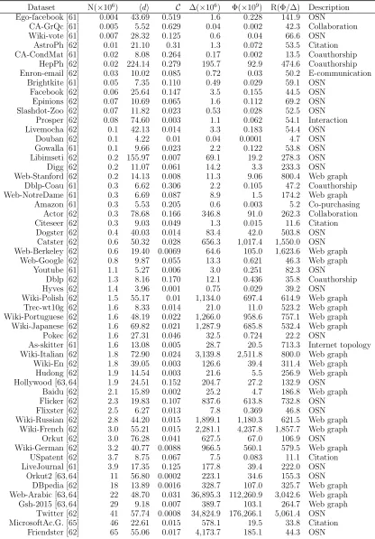
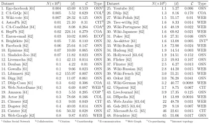
TABLE 2.2: Properties of the networks in our experiments, sorted by graph size N.
Dataset N(×106) hdi C ∆(×106) Φ(×109) R(Φ/∆) Description
Ego-facebook [61] 0.004 43.69 0.519 1.6 0.228 141.9 OSN
CA-GrQc [61] 0.005 5.52 0.629 0.04 0.002 42.3 Collaboration Wiki-vote [61] 0.007 28.32 0.125 0.6 0.04 66.6 OSN
AstroPh [62] 0.01 21.10 0.31 1.3 0.072 53.5 Citation CA-CondMat [61] 0.02 8.08 0.264 0.17 0.002 13.5 Coauthorship
HepPh [62] 0.02 224.14 0.279 195.7 92.9 474.6 Coauthorship Enron-email [62] 0.03 10.02 0.085 0.72 0.03 50.2 E-communication
Brightkite [61] 0.05 7.35 0.110 0.49 0.029 59.1 OSN Facebook [62] 0.06 25.64 0.147 3.5 0.155 44.5 OSN Epinions [62] 0.07 10.69 0.065 1.6 0.112 69.2 OSN Slashdot-Zoo [62] 0.07 11.82 0.023 0.53 0.028 52.5 OSN
Prosper [62] 0.08 74.60 0.003 1.1 0.062 54.1 Interaction Livemocha [62] 0.1 42.13 0.014 3.3 0.183 54.4 OSN
Douban [62] 0.1 4.22 0.01 0.04 0.0001 4.7 OSN Gowalla [61] 0.1 9.66 0.023 2.2 0.122 53.8 OSN Libimseti [62] 0.2 155.97 0.007 69.1 19.2 278.3 OSN Digg [62] 0.2 11.07 0.061 14.2 3.3 233.3 OSN Web-Stanford [62] 0.2 14.13 0.008 11.3 9.06 800.4 Web graph
Dblp-Coau [61] 0.3 6.62 0.306 2.2 0.105 47.2 Coauthorship Web-NotreDame [61] 0.3 6.69 0.087 8.9 1.5 174.2 Web graph
Amazon [61] 0.3 5.53 0.205 0.6 0.003 5.2 Co-purchasing Actor [62] 0.3 78.68 0.166 346.8 91.0 262.3 Collaboration Citeseer [62] 0.3 9.03 0.049 1.3 0.015 11.6 Citation
Dogster [62] 0.4 40.03 0.014 83.4 42.0 503.8 OSN Catster [62] 0.6 50.32 0.028 656.3 1,017.4 1,550.0 OSN Web-Berkeley [62] 0.6 19.40 0.0069 64.6 105.0 1,623.6 Web graph
Web-Google [62] 0.8 9.87 0.055 13.3 0.621 46.3 Web graph Youtube [61] 1.1 5.27 0.006 3.0 0.251 82.3 OSN
Dblp [62] 1.3 8.16 0.170 12.1 0.436 35.8 Coauthorship Hyves [62] 1.4 3.96 0.001 0.75 0.029 39.2 OSN
Wiki-Polish [62] 1.5 55.17 0.01 1,134.0 697.4 614.9 Web graph Trec-wt10g [62] 1.6 8.33 0.014 21.0 11.0 523.2 Web graph Wiki-Portuguese [62] 1.6 48.19 0.022 1,266.0 958.6 757.1 Web graph Wiki-Japanese [62] 1.6 69.82 0.021 1,287.9 685.8 532.4 Web graph
Pokec [62] 1.6 27.31 0.046 32.5 0.724 22.2 OSN
As-skitter [61] 1.6 13.08 0.005 28.7 20.5 713.3 Internet topology Wiki-Italian [62] 1.8 72.90 0.024 3,139.8 2,511.8 800.0 Web graph
Wiki-En [62] 1.8 39.05 0.003 126.6 39.4 311.4 Web graph Hudong [62] 1.9 14.54 0.003 21.6 5.5 256.9 Web graph Hollywood [63, 64] 1.9 24.51 0.152 204.7 27.2 132.9 OSN
Baidu [62] 2.1 15.89 0.002 25.2 4.7 186.8 Web graph Flicker [62] 2.3 19.83 0.107 837.6 613.8 732.8 OSN Flixster [62] 2.5 6.27 0.013 7.8 0.369 46.8 OSN Wiki-Russian [62] 2.8 44.20 0.015 1,899.1 1,180.3 621.5 Web graph
Wiki-French [62] 3.0 55.21 0.015 2,281.1 4,237.8 1,857.7 Web graph Orkut [62] 3.0 76.28 0.041 627.5 67.0 106.9 OSN Wiki-German [62] 3.2 40.77 0.0088 966.5 560.1 579.5 Web graph
USpatent [62] 3.7 8.75 0.067 7.5 0.083 11.1 Citation LiveJournal [61] 3.9 17.35 0.125 177.8 39.4 222.0 OSN
Orkut2 [63, 64] 11 56.80 0.0002 223.1 34.6 155.3 OSN DBpedia [62] 18 13.89 0.0016 328.7 107.0 325.7 Web graph Web-Arabic [63, 64] 22 48.70 0.031 36,895.3 112,260.9 3,042.6 Web graph Gsh-2015 [63, 64] 29 9.18 0.007 389.7 103.1 264.7 Web graph
Twitter [62] 41 57.74 0.0008 34,824.9 176,266.1 5,061.4 OSN MicrosoftAc.G. [65] 46 22.61 0.015 578.1 19.5 33.8 Citation
2.4
Experiments
Our analytical results are derived with approximations based on the assumption on
the data size and sample size. The experiments are designed to confirm the validity of
the analytical results, and empirically demonstrate how much better our method is.
In particular, analytical results do not include the cost of additional closeness check.
These experiments confirm that such cost does not affect our overall result.
2.4.1
Datasets
We used 56 real world graphs to evaluate the algorithms, whose statistics are
summa-rized in Table 2.2. We removed repeated edges and self-loops, and ignored the edge
directionality in directed networks. Therefore, some statistics may be different from
other papers working on the same datasets. For example, we found that the Twitter
contains 18% repeated edges. Such repeated edges have to be removed to guarantee
the accuracy of the sampling.
We included almost all the largest graphs that we could find. Examples are
the most recent academic citation graph released by Microsoft, which contains 46
million nodes, and the well-known Twitter user network that has 41 million nodes.
In addition to these large graphs, we also included some smaller graphs of various
scales for comparison. The types of the graphs are also diversified, covering various
areas. There are web graphs, online social networks, citation graphs, co-author and
co-purchasing relations etc.
The experiments are conducted on two servers with 256GB memory and 24 cores
each. The data and code are available on the website http://etemadir.myweb.cs.
uwindsor.ca/cikm2016/triangles.php.
2.4.2
Experimental setup
We verify Theorems 1 and 2 by comparing observed RSEs obtained from running
obtain observed RSE, we repeat the estimation k times using the same sample size,
each time obtain an estimate ∆i. Letµ= 1k Pk
i=1∆i. The observed RSE is calculated
using
RSE = 1 ∆
r 1
k
X
(∆i−µ)2. (16)
In our experiments, k = 1000 for all garphs.
For the sample size parameter, most existing methods, such as Doulion [7], use
a fixed range of sampling probability p or percentages of the edges sampled for all
graphs. Fixed percentage creates a wide variation for RSEs: one percent of sample
data may not be enough to have an accurate estimate for small graphs, but can achieve
very good (small) RSE for large graphs. Instead of fixed percentage, we target at a
fixed range of RSEs, and choose the sample size that can create the RSEs at the
desired range. RSE can reflect the confidence interval of the estimates, which is the
main concern of any estimator.
All the experiments target RSEs between the range of 0.05 and 0.4. Next, we
need to select sample sizen so that the observed RSE would be in that range. Recall
that from Eq.s 10 and 11 we can derive ∆g and ∆|g from desired RSEs. However, we
still do not know what is the sample size n to obtain that number of triangles. We
derived the following theorem to decide the sample size for EG.
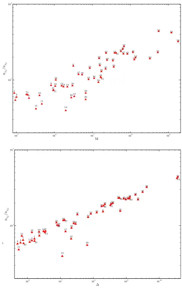
Theorem 3. In EG sampling, the relationship between nEG and ∆|g is
nEG ≈
3N∆|g 2CΓ
12
, (17)
where C is the clustering coefficient, and Γ =CV2+ 1, where CV is the coefficient of
degree variation.
1e−03 7e−03 1e−02 0.1 0.2 0.3 Ego-facebook R S E
8e−03 4e−02 7e−02
CA-GrQc
2e−03 1e−02 2e−02
Wiki-Vote
1e−03 1e−02 2e−02
AstroPh
4e−03 2e−02 3e−02
CA-CondMat
1e−04 7e−04 1e−03
HepPh
2e−03 9e−03 2e−02
Enron-email
2e−03 1e−02 2e−02
Brightkite
8e−04 5e−03 8e−03 0.1 0.2 0.3 Facebook R S E
1e−03 1e−02 2e−02
Epinions
2e−03 2e−02 4e−02
Slashdot-Zoo
2e−03 1e−02 2e−02
Prosper
8e−04 5e−03 9e−03
Livemocha
8e−03 4e−02 7e−02
Douban
1e−03 7e−03 1e−02
Gowalla
2e−04 1e−03 2e−03
Libimseti
4e−04 4e−03 7e−03 0.1 0.2 0.3 Digg R S E
7e−04 1e−02 3e−02
Web-Stanford
1e−03 5e−03 8e−03
Dblp-Coau
2e−03 7e−03 1e−02
Amazon
8e−05 4e−04 7e−04
Actor
5e−04 3e−03 5e−03
Web-NotreDame
1e−03 5e−03 9e−03
Citeseer
2e−04 8e−04 1e−03
Dogster
6e−05 5e−04 1e−03 0.1 0.2 0.3 Catster R S E
3e−04 5e−03 9e−03
Web-Berkeley
4e−04 2e−03 3e−03
Web-Google
9e−04 4e−03 7e−03
Youtube
4e−04 2e−03 3e−03
Dblp
2e−03 1e−02 2e−02
Hyves
4e−05 2e−04 4e−04
Wiki-Polish
4e−04 5e−03 1e−02
Trec-wt10g
4e−05 2e−04 4e−04 0.1 0.2 0.3 Wiki-Portuguese R S E
4e−05 2e−04 4e−04
Wiki-Japanese
3e−04 1e−03 2e−03
Pokec
3e−04 2e−03 3e−03
As-skitter
3e−05 1e−04 2e−04
Wiki-Italian
1e−04 8e−04 1e−03
Wiki-En
4e−04 3e−03 5e−03
Hudong
1e−04 5e−04 8e−04
Hollywood
3e−04 2e−03 4e−03 0.1 0.2 0.3 Baidu R S E
5e−05 2e−04 4e−04
FLicker
5e−04 3e−03 5e−03
Flixster
3e−05 2e−04 3e−04
Wiki-Russian
3e−05 2e−04 4e−04
Wiki-Franch
6e−05 2e−04 4e−04
Orkut
5e−05 3e−04 5e−04
Wiki-German
5e−04 2e−03 4e−03
USpatent
1e−04 5e−04 9e−04 0.1 0.2 0.3 LiveJournal R S E
pE G
1e−04 4e−04 7e−04
Orkut2
pE G
8e−05 4e−04 8e−04
DBpedia
pE G
8e−06 3e−05 6e−05
Web-Arabic
pE G
8e−05 4e−04 7e−04
Gsh-2015
pE G
8e−06 4e−05 6e−05
pE G
6e−05 2e−04 4e−04
MicrosoftAG
pE G
2e−05 9e−05 2e−04
Friendster
pE G
Obs. Est.
FIGURE 2.3: The observed and estimated RSEs of estimator EG. Estimated values are obtained from Eq. 10.
between N and the sample subgraph g as follows:
N = 1
wg
n
2
Γ. (18)
Here, n = 2×nEg is the total number of times the nodes have been sampled. It is
the sum of all the degrees of the sample graph g, or number of edges times two. wg
is the number of collisions in [11], which can be interpreted as the number wedges in
g. After rearranging the above formula, we have:
n2−n = 2N wg
Γ . (19)
Recall that wg = 3∆
|g