with Improved Aerosol Activation and Cloud Parameterizations. (Under the direction of Dr. Yang Zhang).
A new 3-D model testbed for air quality and climate related research over East Asia
has been established through conducting simulations using the Weather Research and
Forecasting model couple with online chemistry. January, April, July, and October 2005 that
represent four seasons have been selected for the simulation. Multiple observational datasets
from air quality monitoring agencies in China, Hong Kong, Taiwan, Japan, and satellites
have been used to perform a comprehensive evaluation for the purpose of improving model
capability and reducing uncertainties and errors in the model input files. A new modeling
system, the Weather Research and Forecasting model coupled with the Community
Atmospheric Model version 5 (WRF-CAM5) has been recently developed for regional
climate research. An advanced cloud parameterization that allows aerosol-cloud interactions
in the convective clouds has been incorporated into WRF-CAM5 by Pacific Northwest
Nation Laboratory. In this study, a comprehensive evaluation is performed to assess the
capability of WRF-CAM5 in representing current atmosphere.
An advanced aerosol activation parameterization incorporated in the WRF-CAM5. It
is based on Fountoukis and Nenes (2005) (referred to as FN05) and a series updated features
including the treatment of kinematic limitations of Giant CCN (Barahona et al., 2010)
(referred to as B10), the effect from convective entrainment (Barahona and Nenes, 2007)
(referred to as BN07), and the adsorptive activation pathway for insoluble particles (Kumar
et al., 2009) (referred to as K09). Aerosol activation that is the crucial link of cloud aerosol
and widely used Abdul-Razzack Ghan (2000) parameterization (referred to as AR-G00),
FN05 gives ~130% higher non-convective CDNC, and together with other new features
gives ~160% higher non-convective CDNC. FN05 series of parameterization also agree
better with satellite derived CDNC based on Bennartz et al. (2007). Further investigation
shows that half of the increase in non-convective CDNC could be attributed to the higher
aerosol activation fraction by FN05 series than that by AR-G00, and remaining half of the
difference could be due to the feedbacks in subsequent cloud microphysics. The changes in
cloud properties have further impact on the radiation and precipitation. Simulations with
FN05 series give ~2% lower SWDOWN and ~5% lower precipitation that those from
© Copyright 2013 by Xin Zhang
by Xin Zhang
A thesis submitted to the Graduate Faculty of North Carolina State University
in partial fulfillment of the requirements for the degree of
Master of Science
Marine, Earth and Atmospheric Sciences
Raleigh, North Carolina
2013
APPROVED BY:
_______________________________ ______________________________
Dr. Markus Petters Dr. Shaocai Yu
Co-Chair of Advisory Committee
________________________________ Dr. Yang Zhang
BIOGRAPHY
Xin Zhang was born and raised in Beijing, China. When he was young, he had developed
interest in the nature and later on the natural sciences. He went to Peking University to study
Environmental Sciences after high school. During the 3rd year of his undergraduate study
supported by the undergraduate research project he joined the atmospheric chemistry
research group at the university and began to work on atmospheric pollutant monitoring and
composition analysis. He learned the importance of scientific research to the atmospheric
pollution control through his undergraduate research project. He applied the graduate
program at NC state university in fall 2011. Since spring 2012 he started working on the
regional atmospheric modeling over East Asia with a focus on China in Dr. Yang Zhang’ Air
ACKNOWLEDGMENTS
I would like to thank my graduate committee members Drs. Yang Zhang, Shaocai Yu, and
Markus Petters for their strong support when I have difficulties during this study, and in
particular my advisor, Dr. Yang Zhang.
I would like to thanks the U.S. Department of Energy (Grant number: DE-SC0006695) and
the U.S. NSF FaSM program (AGS-1049200) for supporting this project. I also want to thank
our collaborators, including Drs. Jiwen Fan, L. Ruby Leung and K.-S. Lim from the Pacific
Northwest National Laboratory for providing the WRF-CAM5 modeling system, and Dr.
Athanasios Nenes from Georgia Institute of Technology for providing the FN05 series
aerosol activation source code.
I’ve received numerous help from members of the Air Quality Forecasting Lab group
members: Dr. Kai Wang, Dr. Brett Gantt, Dr. Shuai Zhu, Changjie Cai, Tim Glotfelty,
Ashley Penrod, Jian He, Khairunnisa Yahya, LeeAnna Chapman, Wei Wang, and Ying
Chen.
TABLE OF CONTENTS
LIST OF TABLES ... vii
LIST OF FIGURES ...x
LIST OF ABBREVIATIONS ... xvi
CHAPTER 1. INTRODUCTION ...1
1.1 Background and Motivation ...1
1.2 Overall Technical Approaches and Objectives ...3
1.3 Literature Review ...5
1.3.1 Climate Change and Aerosol Effects ...5
1.3.2 Aerosol Activation Parameterizations ...7
1.3.3 Cloud Parameterizations ...10
1.4 Model Description ...11
1.4.1 WRF/Chem ...11
1.4.2 WRF-CAM5 ...12
1.5 Domain and Episode Description ...12
CHAPTER 2. ESTABLISHMENT OF EAST ASIA SIMULATION TESTBED THROUGH WRF/CHEM SIMULATIONS ...17
2.1 WRF/Chem Model Inputs, Configurations, and Simulation Design ...17
2.2 Observational Datasets and Model Evaluation Protocols ...20
2.3 Improvements in Model Inputs and Treatments ...25
2.3.1 Adjustment of Anthropogenic Emissions ...27
2.3.2 Improvement in Online Dust Emissions ...27
2.3.4 Treatment of Secondary Organic Aerosols ...31
2.3.5 Adjustment of Ozone Boundary Conditions ...31
2.4 Model Evaluation of WRF/Chem ...32
2.4.1 Baseline Simulations ...33
2.4.2 Sensitivity Simulations ...38
CHAPTER 3. INCORPORATION OF IMPROVED AEROSOL ACTIVATION PARAMETERIZATION INTO WRF-CAM5 ...72
3.1 Representation of Aerosols in WRF-CAM5 ...72
3.2 Incorporation of FN05 and Its Updates into WRF-CAM5 ...74
3.2.1 Overview ...74
3.2.2 Steps of Calculation and Coding Structure ...75
3.3 Differences between AR-G00 and FN05 Parameterizations ...88
CHAPTER 4. WRF-CAM5 SIMULATIONS WITH DIFFERENT AEROSOL ACTIVATION PARAMETERIZATIONS ...105
4.1 WRF-CAM5 Model Configurations ...105
4.2 Evaluation Protocols and Observational Datasets ...106
4.3 Evaluation of WRF-CAM5 Simulation Results ...108
4.3.1 Meteorological Variables ...108
4.3.2 Surface Chemical Concentration ...110
4.3.3 Column Mass Abundance ...112
4.3.4 Aerosol and Cloud Variables ...113
4.4 Intercomparison of Different Aerosol Activation Parameterization ...114
4.4.2 Convective Cloud ...116
4.4.3 Radiation and Precipitation ...117
CHAPTER 5. SUMMARY AND CONCLUSIONS ...164
LIST OF TABLES
Table 2.1. WRF/Chem Model Components and Configurations ... 18
Table 2.2. Parameters and Associated Observational Databases Included in the Model Evaluation: Surface Databases ... 21
Table 2.3. Parameters and Associated Observational Databases Included in the Model Evaluation: Satellite Databases ... 23
Table 2.4. and Sensitivity Simulations Using WRF/Chem ... 28
Table 2.5. Emissions Adjustment Factors Used in ADJEMIS1 ... 29
Table 2.6. Emissions Adjustment Factors Used in ADJEMIS2 ... 30
Table 2.7. Performance Statistics for Meteorological Variables from WRF/Chem Simulation ... 43
Table 2.8. Performance Statistics for Surface and Column CO from WRF/Chem Simulations ... 45
Table 2.9. Performance Statistics for Surface and Column NO2 from WRF/Chem Simulations ... 47
Table 2.10. Performance Statistics for Surface NO from WRF/Chem Simulations ... 49
Table 2.11. Performance Statistics for Surface and Column SO2 from WRF/Chem Simulations ... 50
Table 2.12. Performance Statistics for Surface O3 and Tropospheric Ozone Column from WRF/Chem Simulations ... 52
Table 2.13. Performance Statistics for Surface PM10, PM2.5, and Column AOD from WRF/Chem Simulations ... 54
Table 3.1. Hygroscopicity and Density (kg m-3) of Aerosol Components (Liu et al. 2012) ... 92
Table 3.2. Testing Simulations to Examine Incorporation of FN05 and Explain Difference between AR-G00 and FN05 ... 96
Table 4.2. Parameters and Associated Observational Databases Included in the Model Evaluation: Satellite Databases ... 119 Table 4.3. Baseline and Sensitivity Simulations Conducted Using WRF-CAM5 ... 120 Table 4.4. 2005 Annual Normalized Mean Bias (NMB, %) for Meteorological
and Chemical Variables from the WRF-CAM5 Simulations ... 121 Table 4.5. 2010 Annual Normalized Mean Bias (NMB, %) for Meteorological
and Chemical Variables from the WRF-CAM5 Simulations ... 122 Table 4.6. 2005 Annual Correlation Coefficient for Meteorological and Chemical
Variables from the WRF-CAM5 Simulations ... 123 Table 4.7. 2010 Annual Correlation Coefficient for Meteorological and Chemical
Variables from the WRF-CAM5 Simulations ... 124 Table 4.8. 2005 Winter Seasonal Normalized Mean Bias (NMB, %) for
Meteorological and Chemical Variables from the WRF-CAM5
Simulations ... 125 Table 4.9. 2010 Winter Seasonal Normalized Mean Bias (NMB, %) for
Meteorological and Chemical Variables from the WRF-CAM5
Simulations ... 126 Table 4.10. 2005 Winter Seasonal Correlation Coefficient for Meteorological and
Chemical Variables from the WRF-CAM5 Simulations ... 127 Table 4.11. 2010 Winter Seasonal Correlation Coefficient for Meteorological and
Chemical Variables from the WRF-CAM5 Simulations ... 128 Table 4.12. 2005 Spring Seasonal Normalized Mean Bias (NMB, %) for
Meteorological and Chemical Variables from the WRF-CAM5
Simulations ... 129 Table 4.13. 2010 Spring Seasonal Normalized Mean Bias (NMB, %) for
Meteorological and Chemical Variables from the WRF-CAM5
Simulations ... 130 Table 4.14. 2005 Spring Seasonal Correlation Coefficient for Meteorological and
Chemical Variables from the WRF-CAM5 Simulations ... 131 Table 4.15. 2010 Spring Seasonal Correlation Coefficient for Meteorological and
Table 4.16. 2005 Summer Seasonal Normalized Mean Bias (NMB, %) for Meteorological and Chemical Variables from the WRF-CAM5
Simulations ... 133 Table 4.17. 2010 Summer Seasonal Normalized Mean Bias (NMB, %) for
Meteorological and Chemical Variables from the WRF-CAM5
Simulations ... 134 Table 4.18. 2005 Summer Seasonal Correlation Coefficient for Meteorological and
Chemical Variables from the WRF-CAM5 Simulations ... 135 Table 4.19. 2010 Summer Seasonal Correlation Coefficient for Meteorological and
Chemical Variables from the WRF-CAM5 Simulations ... 136 Table 4.20. 2005 Autumn Seasonal Normalized Mean Bias (NMB, %) for
Meteorological and Chemical Variables from the WRF-CAM5
Simulations ... 137 Table 4.21. 2010 Autumn Seasonal Normalized Mean Bias (NMB, %) for
Meteorological and Chemical Variables from the WRF-CAM5
Simulations ... 138 Table 4.22. 2005 Autumn Seasonal Correlation Coefficient for Meteorological and
Chemical Variables from the WRF-CAM5 Simulations ... 139 Table 4.23. 2010 Autumn Seasonal Correlation Coefficient for Meteorological and
LIST OF FIGURES
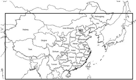
Figure 1.1. The WRF/Chem and WRF-CAM5 modeling domain at a horizontal grid
resolution of 36-km (97×164 cells) (Wang et al., 2010). ... 14 Figure 1.2. Domain-wide annul mean value of air pollution index (API) reported by
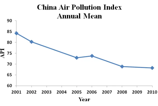
the Ministry of Environmental Protection of the People's Republic of China for years 2001, 2002, 2005, 2006, 2008, and 2010. ... 15 Figure 1.3. Domain-wide summer seasonal mean value of the National Climatic
Data Center (NCDC) daily precipitation for years 2001, 2002, 2005, 2006, 2008, and 2010. ... 16 Figure 2.1. Map of locations of observational sites. (a) NCDC sites (blue dots), (b)
China-API (blue dots), Japan-NIES (green dots), Taiwan-PSI (yellow dots), Hong Kong-API (purple pentagram), and THU-PM (red pentagram). .. 22 Figure 2.2. Time series of surface concentration of CO, NO, NO2, SO2, O3 and PM10
in Hong Kong from Observations (Hong Kong-API, in blue), ORIGEMIS (in green), ADJEMIS1 (in black), ADJEMIS2 (in red), WCoff, and
SOAoff (in purple). ... 56 Figure 2.3. Time series and chemical compositions of PM2.5 in Tsinghua University
(THU), Beijing from Observations (in blue), ORIGEMIS (in green), ADJEMIS1 (in black), ADJEMIS2 (in red), and WCoff and SOAoff (in
purple). ... 59 Figure 2.4. Time series and chemical compositions of PM2.5 in Miyun, Beijing from
Observations (in blue), ORIGEMIS (in green), ADJEMIS1 (in black),
ADJEMIS2 (in red), and WCoff and SOAoff (in purple). ... 60 Figure 2.5. AOD from MODIS (raw 1), ORIGEMIS (raw 2), ADJEMIS1 (raw 3)
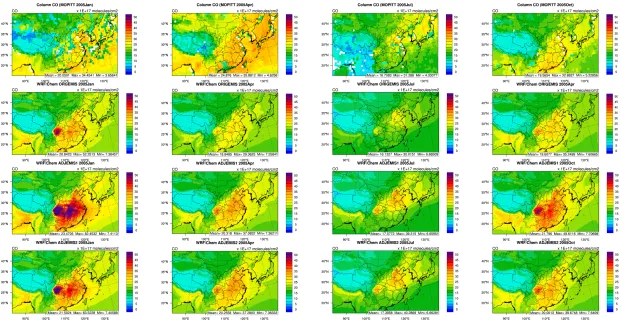
and ADJEMIS2 (raw 4) for January (column 1), April (column 2), July (column 3), and October (column 4) 2005. ... 61 Figure 2.6. CO column from MOPITT (raw 1), ORIGEMIS (raw 2), ADJEMIS1
(raw 3) and ADJEMIS2 (raw 4) for January (column 1), April (column 2), July (column 3), and October (column 4) 2005. ... 62 Figure 2.7. Tropospheric ozone column from OMI (raw 1), TOMS(raw 2),
ORIGEMIS (raw 3), ADJEMIS1 (raw 4) and ADJEMIS2 (raw 5) for January (column 1), April (column 2), July (column 3), and October
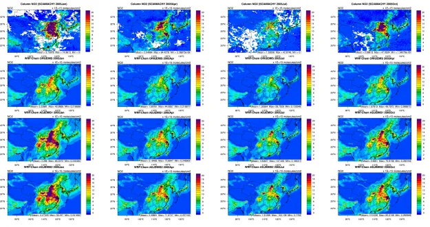
Figure 2.8. NO2 column from SCIAMACHY (raw 1), ORIGEMIS (raw 2),
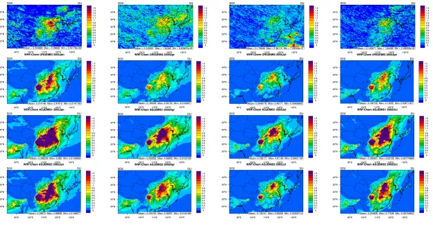
ADJEMIS1 (raw 3) and ADJEMIS2 (raw 4) for January (column 1), April (column 2), July (column 3), and October (column 4) 2005.. ... 66 Figure 2.9. SO2 column from SCIAMACHY (raw 1), ORIGEMIS (raw 2),
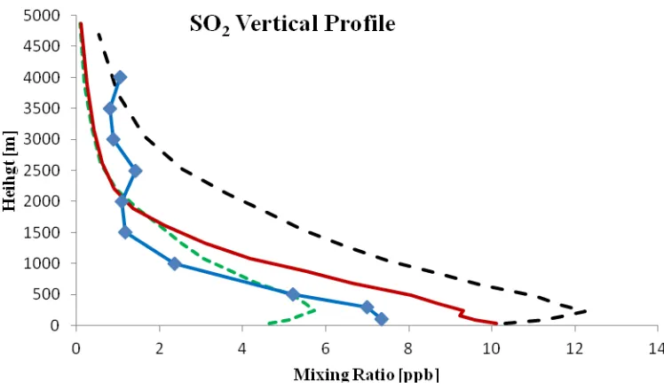
ADJEMIS1 (raw 3) and ADJEMIS2 (raw 4) for January (column 1), April (column 2), July (column 3), and October (column 4) 2005. ... 67 Figure 2.10. SO2 vertical profiles from observation (He et al., 2011, in blue),
ORIGEMIS1 (in green), ADJEMIS1 (in black), and ADJEMIS2 (in red). ... 68 Figure 2.11. The original (blue) and updated (red) O3 boundary conditions. ... 69 Figure 2.12. Surface PM10 concentrations for July 2005 from ORIGEMIS,
ADJEMIS1 and ADJEMIS2 simulations. ... 70 Figure 2.13. Absolute differences of surface OC and PM2.5 concentrations, O3, NO2,
isoprene, and toluene mixing ratios for July 2005 between ADJEMIS2 and SOAoff. ... 71 Figure 3.1. Flow chart of Morrison and Gettelman (2008) microphysics scheme in
WRF-CAM5 with the aerosol activation subroutine in bold font. ... 93 Figure 3.2. Flow chart of Song and Zhang (2011) cumulus scheme in WRF-CAM5
with the aerosol activation subroutine in bold font. ... 94 Figure 3.3. Flow chart of the aerosol activation calculation in ARG00 and FN05 series.. 95 Figure 3.4. Updraft velocity (top) and volume-mean accumulation mode hygrosopicity
(bottom) of the ARG00DEF (left) and FN05DEF (right) from the 2nd
time step and surface layer results. ... 97 Figure 3.5. Updraft velocity (top) and volume-mean accumulation mode hygrosopicity
(bottom) of the ARG00DEF (left) and FN05DEF (right) from the 60th
time step and surface layer results. ... 98 Figure 3.6. Critical supersaturation of accumulation mode simulated by the
ARG00DEF (top-left), ARG00MOD (top-right), FN05DEF (bottom-left), and FN05MOD (bottom-right) from the 2nd time step and surface layer.. ... 99 Figure 3.7. Critical supersaturation of accumulation mode simulated by the
Figure 3.8. Percentage differences in calculated max supersaturation between ARG00MOD and ARG00DEF (top), between FN05MOD and
ARG00MOD (middle), and between FN05DEF and FN05MOD (bottom) from the surface layer at 2nd time step (left) and the 60th time step results.. .. 101
Figure 3.9. Percentage differences in activated number fraction for accumulation mode between ARG00MOD and ARG00DEF (top), between FN05MOD and ARG00MOD (middle), and between FN05DEF and FN05MOD (bottom) from the surface layer at 2nd time step (left) and the 60th time
step results. ... 102 Figure 3.10. Percentage differences in activated number fraction for Aitken mode
between ARG00MOD and ARG00DEF (top), between FN05MOD and ARG00MOD (middle), and between FN05DEF and FN05MOD (bottom) from the surface layer at 2nd time step (left) and the 60th time step results. ... 103 Figure 3.11. Grid point comparison of 2nd time step surface layer max supersaturation
(top), activated number fractions for accumulation mode (middle) and Aitken mode (bottom), (a) between ARG00DEF and ARG00MOD, (b) between ARG00MOD and FN05MOD, (c) between FN05MOD and
FN05DEF, and (d) between ARG00DEF and FN05DEF. ... 104 Figure 4.1. AOD (row 1), COTL (row 2), CWPL (row 3), column CO (row 4),
column NO2 (row 5), tropospheric column O3 (row 6) and column SO2
(row 7) from satellite observations (column 1), AR-G00 (column 2), FN05 (column 3) and FN05/B10/ K09/BN07 (column 4) for 2005. ... 141 Figure 4.2. AOD (row 1), COTL (row 2), CWPL (row 3), column CO (row 4),
column NO2 (row 5), tropospheric column O3 (row 6) and column SO2
(row 7) from satellite observations (column 1), AR-G00 (column 2), FN05 (column 3) and FN05/B10/ K09/BN07 (column 4) for 2010. ... 144 Figure 4.3. Simulated CDNC from (top to bottom) AR-G00, FN05, FN05/B10,
FN05/K09, FN05/BN07, and FN05/B10/K09/BN07 runs for 2005 (left) and 2010 (right). ... 147 Figure 4.4. CDNC between 960 mb to 850 mb from (top to bottom) satellite
Figure 4.5. CDNC between 960 mb to 850 mb from (top to bottom) satellite derivation by Aqua derived by Bennartz (2007) and the WRF-CAM5 simulations with AR-G00, FN05, FN05/B10, FN05/K09, FN05/BN07 and FN05/B10/K09/BN07 for 2005 (left) and 2010 (right). ... 149 Figure 4.6. Percentage differences of non-convective cloud borne aerosols from the
WRF-CAM5 simulations (top to bottom) between each of the FN05 series (i.e., FN05, FN05/B10, FN05/K09, FN05/BN07, FN05/B10/K09/BN07) and AR-G00 for 2005 (left) and 2010 (right). ... 150 Figure 4.7. Percentage differences of non-convective CDNC from the WRF-CAM5
simulations (top to bottom) between each of the FN05 series (i.e., FN05, FN05/B10, FN05/K09, FN05/BN07, FN05/B10/K09/BN07) and AR-G00 for 2005 (left) and 2010 (right). ... 151 Figure 4.8. Percentage differences of convective CCN tendency from the
WRF-CAM5 simulations (top to bottom) between convFN05 and AR-G00, and between convALL and AR-G00 for the summers of 2005 (left) and 2010 (right). ... 152 Figure 4.9. Percentage difference of convective CDNC tendency from the
WRF-CAM5 simulations (top to bottom) between convFN05 and AR-G00, and between convALL and AR-G00 for the summers of 2005 (left) and 2010 (right). ... 153 Figure 4.10. Downward longwave radiation at surface from the CERES satellite
observations (column 1), AR-G00 (column 2), FN05 (column 3) and FN05/B10/ K09/BN07 (column 4) for 2010 annual mean (row 1), winter mean (row 2), spring mean (row 3), summer mean (row 4), and autumn mean (row 5). ... 154 Figure 4.11. Downward longwave radiation at surface from the CERES satellite
observations (column 1), AR-G00 (column 2), FN05 (column 3) and
FN05/B10/ K09/BN07 (column 4) for 2010 annual mean (row 1), winter mean (row 2), spring mean (row 3), summer mean (row 4), and autumn mean (row 5). ... 155 Figure 4.12. Downward shortwave radiation at surface from CERES satellite
Figure 4.13. Downward shortwave radiation at surface from the CERES satellite observations (column 1), AR-G00 (column 2), FN05 (column 3) and FN05/B10/ K09/BN07 (column 4) for 2010 annual mean (row 1), winter mean (row 2), spring mean (row 3), summer mean (row 4), and autumn mean (row 5). ... 157 Figure 4.14. Percentage differences of downward longwave radiation at surface
(row 1), downward shortwave radiation at surface (row 2), total precipitation (row 3), non-convective precipitation (row 4), and
convective precipitation (row 5) between the WRF-CAM5 simulations with FN05 and AR-G00 for 2005 (left) and 2010 (right). ... 158 Figure 4.15. Percentage differences of downward longwave radiation at surface
(row 1), downward shortwave radiation at surface (row 2), total precipitation (row 3), non-convective precipitation (row 4), and convective precipitation (row 5) between the WRF-CAM5 simulations with FN05 and AR-G00 for the summer of 2005 (left) and 2010 (right). ... 159 Figure 4.16. Percentage differences of downward longwave radiation at surface
(row 1), downward shortwave radiation at surface (row 2), total precipitation (row 3), non-convective precipitation (row 4), and convective precipitation (row 5) between the WRF-CAM5 simulations with FN05/B10/ K09/BN07 and AR-G00 for 2005 (left) and 2010 (right). .. 160 Figure 4.17. Percentage differences of downward longwave radiation at surface
(row 1), downward shortwave radiation at surface (row 2), total precipitation (row 3), non-convective precipitation (row 4), and convective precipitation (row 5) between the WRF-CAM5 simulations with FN05/B10/ K09/BN07 and AR-G00 for the summers of 2005 (left) and 2010 (right). ... 161 Figure 4.18. Percentage differences of downward longwave radiation at surface
(row 1), downward shortwave radiation at surface (row 2), total precipitation (row 3), non-convective precipitation (row 4), and
convective precipitation (row 5) between the WRF-CAM5 simulation s with convFN05 and AR-G00 for the summers of 2005 (left) and 2010 (right). ... 162
LIST OF ABBREVIATIONS
Abbreviation Definition
ADJEMIS1 Simulations with 1st adjustment of anthropogenic emissions
ADJEMIS2 Simulations with 2nd adjustment of anthropogenic emissions
AR-G00 Abdul-Razzak and Ghan (2000) aerosol activation
parameterization
AOD Aerosol optical depth
API Air pollution index
B10 Barahona et al. (2010) treatment of giant cloud condensation
nuclei kinetic limitation
BC Boundary condition
BN07 Barahona and Nenes (2007) treatment of convective entrainment
CAM5 Community Atmosphere Model version 5
CBM-Z Carbon-Bond Mechanism version Z
CCN Cloud condensation nuclei
CDNC Cloud droplet number concentration
CMAQ Community Multiscale Air Quality model
CO Carbon monoxide
COTL Liquid cloud optical thickness
CWPL Liquid cloud water path
FTUV Fast Tropospheric Ultraviolet-Visible
GEOS-Chem Global Chemical Transport Model with chemistry
IC Initial condition
IPCC Intergovernmental Panel on Climate Change
K09 Kumar et al. (2009) adsorptive aerosol activation parameterization
MAM Modal aerosol module
MAM3 Modal aerosol module with three aerosol modes
MAM7 Modal aerosol module with seven aerosol modes
MEGAN Model of Emissions of Gases and Aerosols from Nature
MEP Ministry of Environmental Protection of China
MG08 Morrison and Gettelman (2008) cloud microphysics
MODIS MOderate-resolution Imaging Spectroradiometer
MOPITT Measurements of Pollution in the Troposphere
MOSAIC Model for Simulating Aerosol Interactions and Chemistry
NASA National Atmospheric and Space Administration
NCAR National Center for Atmospheric Research
NCDC National Climatic Data Center
NCEP National Centers for Environmental Prediction
NIES National Institute of Environmental Studies
NMB Normalized mean bias
NO Nitrogen monoxide
NO2 Nitrogen dioxide
NOAA National Oceanic and Atmospheric Administration
NOAH National Center for Environmental Prediction, Oregon State
University, Air Force, and Hydrologic Research Lab’s
O3 Ozone
OMI Ozone Monitoring Instrument
ORIGEMIS Simulations with original anthropogenic emissions
PBL Planetary boundary layer
PM Particulate matter
PM10 Particulate matter of diameter less than 10 µm
PM2.5 Particulate matter of diameter less than 2.5 µm
PNNL Pacific Northwest National Laboratory
Q2 Water vapor mixing ratios at 2 meters
RH Relative humidity
RRTM Rapid radiative transfer model
RRTMG Rapid radiative transfer model for GCMs
Sc Critical supersaturation
SCIAMACHY Scanning Imaging Absorption Spectrometer
Smax Maximum supersaturation
SOA Secondary organic aerosols
SOAoff Simulations with secondary organic aerosol formation turned off
SZ11 Song and Zhang (2011) cumulus scheme
T2 Temperature at 2 meter
THU Tsinghua University, China
TOMS Total Ozone Mapping Spectrometer
TOR Tropospheric ozone residue
UTC Coordinated universal time
UW University of Washington
VOCs Volatile organic compounds
WCoff Simulations with wind speed correction turned off
WRF Weather Research and Forecasting model
WRF/Chem Weather Research and Forecasting model with online coupled
chemistry
WRF-CAM5 Weather Research and Forecasting model coupled with the
Community Atmosphere Model version 5
CHAPTER 1. INTRODUCTION
1.1 Background and Motivation
Climate change, due to its large influence on the life and the future of human being,
has received intensive scientific research attentions during the past decades. Despite
considerable knowledge people have gained, large uncertainties remain. An accurate
estimation of the effects of anthropogenic activities on climate change is not yet possible.
Aerosol, the small particle suspends in the air, is one of the major contributors to these
uncertainties because of its complicated role in the atmosphere. Aerosols could scatter or
absorb radiations that directly change global radiation balance, and serve as cloud
condensation nuclei (CCN) to affect cloud formation and cloud properties; they thus have
indirect impacts on the global climate. To understand and assess the climatic impacts of
aerosols, it is necessary to examine the processes that involve in the aerosol-cloud
interactions. The aerosol activation process, which determines the fraction of aerosols that
could serve as CCN and grow into cloud droplets, is the crucial link between aerosol particles
and cloud droplets. Thus the model’s representations of aerosol activation processes could
have potentially large impacts on climate change projections.
Thanks to the rapid development of computational powers, numerical models have
become a powerful tool in the research of atmospheric sciences. Atmospheric processes can
be programmed in such models so that they could be represented in the simulations. By
comparing the simulated results and observations, the credibility of current description of
anthropogenic emissions levels) control experiments could be performed to assess the
impacts from historical policies or predict possible future environments assuming different
emission reduction scenarios.
Recently a variant of the Weather Research and Forecasting model coupled with
chemistry (WRF/Chem) (Grell et al., 2005) that includes the Community Atmospheric Model
version 5 physics suite (Neale et al., 2010, referred to as WRF-CAM5) has been developed
by the Pacific Northwest National Laboratory (PNNL) for regional climate research (Ma et
al., 2013, see section 1.4.2 for more detailed description). WRF-CAM5 includes improved
cloud parameterizations such as an explicit linkage between aerosols and deep convection
and an up-to-date ice-nucleation parameterization in mixed-phase cloud and ice cloud. It
therefore provides a more complete representation of aerosol-cloud interactions. As a newly
developed model, its performance will be evaluated using available observational datasets in
this study. Meanwhile, an alternative aerosol activation parameterization based on
Fountoukis and Nenes (2005) (FN05) with several updates including the treatment of
kinematic limitations of giant CCN (Barahona et al., 2010) (B10), the effect from convective
entrainment (Barahona and Nenes, 2007) (BN07), and the adsorptive activation pathway for
insoluble particles (Kumar et al., 2009) (K09) (referred to as FN05 series here after) have
been incorporated into WRF-CAM5 as an alternative to the default aerosol activation
parameterization based on Abdul-Razzak Ghan (2000) (AR-G00). Long-term regional
examine the climatic impacts of aerosols through the aerosol activation process and other
aerosol direct and indirect pathways.
The selected testbed for WRF-CAM5 will be East Asia domain with a major focus on
China. As a developing country, China has experienced a rapid growth of economy and
associated increases in emission levels in the past three decades, emerging as one of the
largest contributors to global climate change. Meanwhile the complicated weather system in
China provides opportunities for testing the model under various meteorological and
chemical conditions. While WRF-CAM5 is being developed, WRF/Chem is publicly
available and widely used (see section 1.4.1 for more detailed description). In this work,
WRF/Chem is used to build the testbed for further development and application of
WRF-CAM5. By comparing with observational datasets from multiple surface networks and
satellites, results from baseline and sensitivity simulations using WRF/Chem will be
evaluated in order to test the existing model inputs and reduce associated uncertainties for the
further improvements and applications of WRF-CAM5.
1.2 Overall Technical Approaches and Objectives
The overall technical approaches of this study is to utilize two state of the science 3-D
numerical models (WRF/Chem and WRF-CAM5) to examine the current model’s capability
in reproducing the real atmosphere and to examine the sensitivity of the model predictions to
different aerosol activation treatments. Te proposed work involves two major tasks. The first
task is to establish the East Asia testbed through WRF/Chem simulations. The second task is
as an alternative into WRF-CAM5 and examine the climatic impacts of aerosols through
intercomparison of two annual baseline and sensitivity simulations with different aerosol
activation parameterizations. For the first task, best available observational datasets from
surface and satellite are collected to evaluate the simulation results. The evaluation protocols
include performance statistics, spatial and temporal analysis that have been widely used in
previous studies (e.g., Queen et al., 2008). Model inputs and configurations are examined and
adjusted through such evaluations to generate reasonable emission and meteorological fields.
For the second task, FN05 series provided by collaborators at Georgia Institute of
Technology will be incorporated into WRF-CAM5 by adding an interface between original
WRF-CAM5 and the provided code of FN05 series (without changing the internal structure
of FN05 series). Incorporated scheme is assessed through testing simulations and
comparisons with previous studies. Then baseline and sensitivity simulations with different
aerosol activation parameterizations are conducted to examine the climatic impacts of
aerosols. The same evaluation method is used for simulations using WRF/Chem and
WRF-CAM5. Relatively long term (with two full years 2005 and 2010) simulation are performed
to investigate the climatic impacts.
The objectives of this study are as follows:
(1) to establish the East Asia testbed by collecting observational datasets, conducting
WRF/Chem simulations for different seasons and examining the representativeness of the
(2) to incorporate a state-of-art aerosol activation parameterization (i.e., FN05 and its
updates based on B10, BN07 and K09) into WRF-CAM5, and couple it with both
non-convective (i.e., model resolved) cloud microphysics and non-convective (i.e., subgrid) cloud
schemes.
(3) to conduct WRF-CAM5 simulations and evaluate model performance for two
years (2005 and 2010) over East Asia with the default aerosol activation parameterization of
AR-G00 and the newly implemented parameterization of FN05 series.
(4) to examine the sensitivity of the model predictions of cloud properties, radiation
and precipitation to different aerosol activation parameterizations through the
intercomparison of 2-year WRF-CAM5 simulation results.
1.3 Literature Review
In this section, a literature review is conducted towards a better understanding of the
role of atmospheric aerosols in climate change, the recent updates of cloud and aerosol
activation parameterizations that are implemented in this study, and the current treatments of
clouds in atmospheric models.
1.3.1 Climate Change and Aerosol Effects
As concluded in the synthesis report by the Intergovernmental Panel on Climate
Change (IPCC) in 2007 (Pachauri et al., 2007), observations have shown that there is a clear
trend of global warming since late 19th century. Global warming is likely to have negative
effects on the habitability of Earth including retreat of glaziers in pole regions, rise of sea
agriculture, as well as a more frequent occurrence of extreme weather events such as
droughts and heavy rainfall. The increasing anthropogenic emissions of greenhouse gases
and their levels in the atmosphere are believed to be the main reason causing global warming.
One of the largest uncertainties in scientific research is the climatic impacts of anthropogenic
aerosols, which are believed to be very complicated with various processes involved.
Aerosols can scatter the incoming solar radiation back to the space and hence have a
cooling effect on the Earth (e.g., Myhre, 2009). Some aerosols like black carbon, however,
can be absorbing agents and hence have a warming effect (e.g., Jacobson, 2000). The
scattering and absorbing of solar radiation are the direct effects of aerosols. Aerosols can also
act as cloud condensation nuclei (CCN) and ice nuclei (IN) and therefore affect cloud
physical and optical properties hence the entire global energy budget, which is known as the
aerosol indirect effects. Reflectance of solar radiation could be enhanced due to an increase
in smaller cloud droplets with fixed cloud water amounts (Twomey, 1977). This is defined as
the Twomey or cloud albedo effect. Smaller cloud droplets also decrease the precipitation
efficiency and therefore prolong cloud lifetime (Albrecht, 1989), which is defined as the
cloud lifetime effect. In addition to the number concentration and effective radius, the whole
spectrum of cloud droplets could also be shaped, having an influence on cloud optical
properties and the initiation of precipitation (Liu and Duam, 2002). Known as a semi-direct
effect, the absorption of solar radiation by black carbon may cause the evaporation of cloud
particles and therefore warming effect due to cloud reduction (Hansen et al., 1997).
absorbing aerosols. When absorbing aerosol is situated above the cloud layer, stronger
inversion might be created and cloud-top entrainment will be reduced, resulting in a
shallower and moister boundary layer with a higher liquid water path, which gives negative
radiative forcing (Johnson et al., 2004). In addition to the aerosol direct and semi-direct
effects, and cloud albedo and cloud lifetime effects, a number of other indirect effects have
been proposed, which are summarized in Lohmann and Feichter (2005).
Most recent modeling study conducted by Ghan et al. (2012) decomposed the aerosol
direct, indirect, and semi-direct radiative forcings within the same model and quantified their
magnitudes on a global scale. As shown in their results, anthropogenic aerosol indirect
effects lead to an average radiative forcing of -2 W m-2 for shortwave radiation and radiative
forcing of 0.5 W m-2 for longwave radiation, while the direct and semi-direct effects are very
small, suggesting the dominant role of aerosol indirect effects in global radiative balance.
Such indirect effects largely compensate the global warming trend by greenhouse gases.
These values of estimated aerosol radiative forcings are consistent with those presented by
IPCC (IPCC, 2007).
1.3.2 Aerosol Activation Parameterizations
Cloud droplets cannot form without the presence of CCN. Köhler theory (Köhler,
1936) described how water vapor condenses on particles and determined whether a dry
particle with certain size and chemical compositions could be activated as CCN at a given
water vapor supersaturation level. As summarized in Ghan et al. (2011), analytical solutions
and chemical properties is present because of the high complexity. However, accurate
numerical solutions under such circumstances could be achieved by dividing aerosols into a
large number of sub-groups that aerosol properties are homogenous within each group. Yet it
is not realistic to obtain such numerical solutions in current global or regional model
simulations since it is extremely computational expensive. The early attempts to build the
linkage between aerosols and cloud droplets were based on empirical relationships, which
have large limitations in their applicability. Physically-based aerosol activation
parameterizations were developed in order to solve CCN concentration accurately and
efficiently in climate research under various conditions. AR-G00 and FN05 are the mostly
used among all the existing aerosol activation parameterizations. Abdul-Razzak et al. (1998)
have developed their aerosol activation parameterization for single aerosol type with
lognormal size distribution, and extended it for multiple externally-mixed lognormal modes
with each mode of soluble and insoluble material internally-mixed (i.e., AR-G00), and for
sectional representation of aerosols (Abdul-Razzak and Ghan, 2002) (AR-G02). On the other
hand, Nenes and Seinfeld (2003) have developed their aerosol activation parameterization
(NS03 parameterization here after) for a sectional representation of aerosol size distribution
using a different approach from that used by AR-G02. FN05 extended NS03
parameterization to allow solving lognormal aerosol distributions and includes the
size-dependent mass transfer coefficient for the growth of water droplet. Nenes and Seinfeld
(2003) compared NS03 with AR-G00 and have found that NS03 gave better agreement with
agreement with numerical solutions than NS03. In the comparison of AR-G00 and FN05
performed by Ghan et al. (2011), FN05 is of higher consistency with numerical solutions
than AR-G00 in predicting the number fraction of activated aerosols. There are several
reasons. First, NS03 and FN05 split aerosols into two populations, one group with diameters
that is activated near maximum supersaturation and another group with diameters that is not
activated near maximum supersaturation. Maximum supersaturation could be calculated
explicitly through limited iterations, so that it could be more accurate than the one by
AR-G00 in which it is calculated through an empirical relationship. Second, NS03 and FN05 treat
the kinetic limitations that may occur for particles having critical supersaturation close to the
maximum supersaturation. Such particles may eventually evaporate and deactivate because
they cannot grow beyond critical size within a short time when air parcel reaches maximum
supersaturation. Third, FN05 includes the size-dependent mass transfer coefficient for the
growth of water droplet. Such treatments are not considered in AR-G00 and NS03. As a
consequence of adding such complexity, FN05 requires 20% more time to be completed than
AR-G00 (Ghan et al., 2011).
Several updates such as the treatment of B10, BN07 and K09 have been incorporated
into the FN05 parameterization. B10 treats the kinematic limitations for giant CCN, namely,
the slow condensation and growing rates are considered for very large particles. Instead of
growing instantaneously, such large particles could also compete for water vapors so that a
reduction in maximum supersaturation would be expected (Barahona et al., 2010). BN07
rising air (Barahona and Nenes, 2007). K09 includes an adsorptive activation mechanism for
the insoluble particles (e.g., dust and black carbon), which is a pathway that is paralleled to
Köhler activation where the surface of the particles is occupied by soluble matters (Kumar et
al., 2009). K09 is based on the multilayer Frenkel-Halsey-Hill (FHH) adsorption isotherm
model with modification to account for particle curvature (Sorjamaa and Laaksonen, 2007).
Compared with the most studied monolayer Langmuir adsorption isotherm model (Langmuir,
1916), FHH model is more applicable to atmospheric particle where multiple layers of water
vapor could be formed. By using K09 an increase in the number faction of activated aerosols
is expected, and the degree of increase depends on the fraction of insoluble particles.
1.3.3 Cloud Parameterizations
Currently cloud parameterizations in most large-scale models are divided into two
sub-divisions, convective and stratiform clouds (also referred to as subgrid and model
resolved clouds, respectively). Microphysics processes in stratiform clouds have been
significantly improved. In the latest version of the National Center for Atmospheric Research
(NCAR) Community Atmosphere Model version 5 (CAM5), mass mixing ratios and number
concentrations (i.e., the two-moment scheme) of four hydrometeors (cloud droplets, cloud
ice, rain, and snow) have been explicitly treated based on Morrison and Gettelman (2008)
(MG08), which allows the simulation of full aerosol-cloud interactions in large-scale clouds.
In convective clouds, however, the microphysics is highly parameterized. The complete
aerosol-cloud-precipitation interactions could not be critically assessed when an explicit
Zhang-MacFarlane (ZM) convective scheme (Zhang and MacFarlane, 1995) in CAM5, a
two-moment scheme similar to MG08 with modifications to suit for convective clouds has
been developed by Song and Zhang (2011) (SZ11) and incorporated into WRF-CAM5 by
PNNL.
1.4 Model Description
Both models (WRF/Chem and WRF-CAM5) used in this study are built on the
structure of the Weather Research and Forecasting model (WRF) that is a next-generation
mesoscale numerical weather prediction system designed to serve both atmospheric research
and operational forecasting needs. WRF incorporates the work from many researchers and
contributors and currently is primarily supported and maintained by the Mesoscale and
Microscale Meteorology Division of NCAR. As suggested in the WRF users’ guide, WRF is
suitable for use in a broad range of applications across scales ranging from meters to
thousands of kilometers, such as urban/regional air quality and regional climate research.
1.4.1 WRF/Chem
The primary goal of designing online-coupled WRF/Chem is to include the
interactions between meteorology and chemistry. By including a chemistry package and
bridging it with the physics, the impact of chemistry on weather and climate could be
represented in the model (Grell et al., 2005). Previous offline atmospheric chemistry models
require meteorological fields as inputs, so there is only one-way impact from meteorology to
from the community. In this study, WRF/Chem version 3.3.1 (released in Sept. 2011) is used
for simulations to develop the modeling testbed.
1.4.2 WRF-CAM5
WRF-CAM5 is a variant of WRF/Chem based on WRF/Chem version 3.4.1 that is
currently under development by PNNL. The CAM5 model physical and chemical schemes
are incorporated into WRF/Chem as an additional option. CAM5 is originally the
atmospheric component in the global model Community Earth System Model (CESM).
WRF-CAM5 is designed to enrich regional climate research, and test the performance of
parameterizations, and investigate atmospheric processes in a multi-scale framework.
WRF-CAM5 includes the up-to-date physics, such as the University of Washington (UW)
planetary boundary layer (PBL) scheme (Bretherton and Park, 2009), the MG08 cloud
microphysics and the ZM convective scheme with SZ11 modifications, which allows the
simulation of full aerosol-cloud interactions.
1.5 Domain and Episode Description
The simulation domain is adopted from the one used by Wang et al. (2010), which is
shown in Figure 1.1. A Lambert projection with the two true latitudes of 25oN and 40oN is
used. The domain origin is (34oN, 110oE), and the coordinates of the southwest corner are x = 2934 km, and y = 1728 km. January, April, July, and October 2005 that represent the four
seasons are selected for the WRF/Chem simulations to establish the modeling testbed. Two
full years, 2005 and 2010, are chosen for WRF-CAM5 simulations among six available years
investigate the climatic impacts from aerosol activation parameterization. According to
Wang et al. (2010), 2005 and 2010 are the end year of the 10th and 11th Five Year Plan, respectively. The expected changes on emissions due to emission control policies could add
more varieties on the simulations. Also as in Figure 1.2, comparison of observational data
from China air pollution index (API) shows that there is a decreasing trend of concentrations
of air pollutants from 2001 to 2010. Meanwhile, precipitation measurements from National
Climatic Data Center (NCDC) also showed that 2005 and 2010 have high summer
precipitation amount among the six available years, which are suitable for this work that
CHAPTER 2. ESTABLISHMENT OF EAST ASIA SIMULATION TESTBED THROUGH WRF/CHEM SIMULATIONS
2.1 WRF/Chem Model Inputs, Configurations, and Simulation Design
Four-month (January, April, July and October 2005) simulations using WRF/Chem
version 3.3.1 are conducted at a grid resolution of 36-km over the East Asia domain. The
model inputs, components, and configurations are summarized in Table 2.1. Same or similar
physical and chemical options have been selected by previous studies (Zhang et al. 2010,
2012). The gas-phase chemistry is based on the Carbon Bond Mechanism-Z (CBM-Z)
(Zaveri and Peters, 1999). The aerosol module is the Model for Simulating Aerosol
Interactions and Chemistry (MOSAIC) (Zaveri et al., 2008). A main reason of using such
combination is that in WRF/Chem version 3.3.1, when CBM-Z and MOSAIC are selected,
aerosol direct and indirect effects (aerosols act as CCN in stratiform clouds) can only be
simulated using the combination of the Goddard shortwave radiation scheme (Chou et al.,
1998), Fast-J photolysis scheme (Wild et al., 2000), the Purdue Lin microphysics (Lin et al.,
1983; Chen and Sun, 2002).
The option of eight sectional aerosol bins with aqueous chemistry for MOSAIC
aerosol module is used in this study to represent aerosol size distribution. The particle size
distribution is represented by 8 bins ranging from 0.0390625 to 10 μm with the first six bins
for PM2.5 and two bins for PM2.5-10. Sulfate (SO42-), nitrate (NO3-), chloride (Cl-), ammonium
(NH4+), sodium (Na+), black carbon (BC), primary organic mass (OC), other inorganic mass
Table 2.1. WRF/Chem Model Components and Configurations
Simulation Period January, April, July, October 2005
Domain East Asia
Horizontal resolution 36 km
Vertical resolution 23 layers from 1000 to 100 mb, with 8 layers in PBL
Meteorological IC and BC The National Centers for Environmental Predictions Final Analysis (NCEP-FNL) reanalysis data; re-initialization every day, and grid nudging of PBL wind withiout re-initialization
Shortwave radiation Goddard shortwave radiation scheme (Chou et al., 1998)
Longwave radiation The rapid radiative transfer model (RRTM) (Mlawer et al.,
1997)
Land surface Community National Centers for Environmental Prediction
(NCEP), Oregon State University, Air Force, and Hydrologic Research Lab-NWS Land Surface Model (NOAH)
(Chen and Dudhia, 2001; Ek et al., 2003)
Surface layer Monin-Obukhov (Monin and Obukhov, 1954; Janjić, 2001)
PBL Yonsei University Scheme (YSU) (Hong et al., 2006)
Cumulus Grell-Devenyi ensemble (Grell and Devenyi, 2002)
Microphysics Purdue Lin (Lin et al., 1983; Chen and Sun, 2002)
Aerosol activation Abdul-Razzak and Ghan (Abdul-Razzak and Ghan, 2002)
Gas-phase chemistry CBM-Z (Zaveri and Peters, 1999)
Photolysis Fast-J (Wild et al., 2000)
Aerosol module Model for Simulating Aerosol Interactions and Chemistry
(MOSAIC) (Zaveri et al., 2008)
Aqueous-phase chemistry Carnegie Mellon University (CMU) mechanism of Fahey
and Pandis (2001)
Chemical IC Community Multiscale Air Quality (CMAQ) modeling
system (Binkowski and Roselle, 2003; Byun and Schere, 2006)
Chemical BC The Goddard Earth Observing System Atmospheric
Chemistry Transport Model (GEOS-Chem) Anthropogenic emissions Wang et al. (2010) and adjusted version
Biogenic emissions Model of Emissions of Gases and Aerosols from Nature
(MEGAN) version 2 (Guenther et al., 2006)
Dust emissions Shaw et al. (2008), and Wang et al. (2012)
such as binary nucleation, coagulation, condensation, inorganic aerosol thermodynamic
equilibrium, PM formation due to aqueous-phase chemistry, aerosol scavenged by cloud
droplets, and dry and wet deposition. However, the formation of secondary organic aerosols
(SOA) is not simulated in MOSAIC. In WRF/Chem version 3.3.1, MOSAIC aerosols using 4
sectional aerosol bins has been coupled with SAPRC99 chemistry and includes volatility
basis set (VBS) for organic aerosol evolution and SOA formation. But MOSAIC- SAPRC99
does not simulate aerosol direct and indirect effects, so it is not selected. In this work, a
simple treatment of secondary organic aerosols formation is thus added in the CBM-Z and
MOSAIC chemistry option that will be further discussed in section 2.3.4.
Meteorology is reinitialized every day in the WRF/Chem simulations to construct a
better meteorological field. Simulations using grid nudging of winds in the PBL with a
nudging coefficient of 0.0003 but without re-initialization are also conducted for comparison.
The National Centers for Environmental Predictions Final Analysis (NCEP-FNL) reanalysis
data is used to create the initial and boundary conditions. The vertical resolution is
Twenty-three layers from 1000 to 100 mb with eight layers in PBL.
The anthropogenic emissions are based on Wang et al. 2010. The original Volatile
Organic Compounds (VOCs) speciation using the 2005 Carbon Bond Mechanism (CB05) is
re-mapped into CBM-Z speciation. Adjustments are applied on the anthropogenic emissions
based on the simulation results, which is further discussed in section 2.3.1. Biogenic, dust
and sea-salt emissions are treated using online modules. The model of Emissions of Gases
emissions. The original Shaw et al. (2008) dust emissions module is first used and then
replaced by Wang et al. (2012) which is discussed in section 2.3.1. Gong et al. (2002) is used
for the generation of sea-salt emissions.
2.2 Observational Datasets and Model Evaluation Protocols
Evaluation of the model performance is necessary for model development and
applications, especially the climate-related research, where only on the basis of reproducing
reasonably acceptable current atmospheric conditions can we make further investigations to
historical, future, or hypothetical cases. For the purpose of establishing modeling testbed, a
comprehensive evaluation using multiple ground-based observational networks and satellite
observations are conducted.
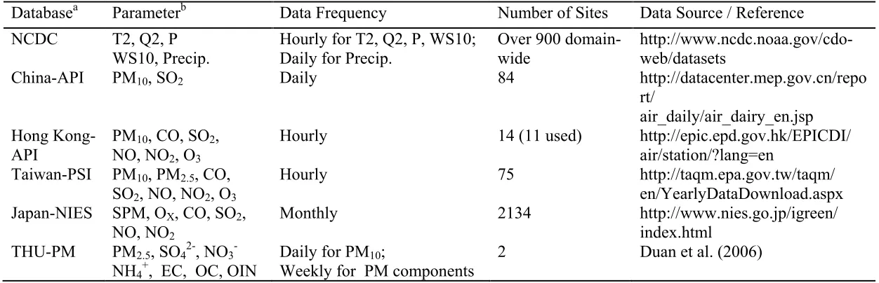
Table 2.2 summarizes the ground-based observational datasets that are collected and
used in this study. Correspondingly, a spatial location map of these observational sites over
the modeling domain is provided in Figure 2.1. The National Climate Data Center (NCDC)
global hourly dataset is used for the evaluation of surface meteorological variables, including
temperature at 2-m (T2), water vapor mixing ratio at 2-m (Q2), surface pressure (P), wind
speed at 10-m (WS10), and daily precipitation (Precip.). Sites that are located outside of our
modeling domain are filtered out. Several observational datasets are collected for the
evaluation of surface chemical variables. PM10 and SO2 concentrations are retrieved for 84
major cities through the Air Pollution Index (API) published by the Chinese Ministry of
Environmental Protection. Observations of PM2.5 and its composition data at a suburban site
Table 2.2. Parameters and Associated Observational Databases Included in the Model Evaluation: Surface Databases
Databasea Parameterb Data Frequency Number of Sites Data Source / Reference
NCDC T2, Q2, P
WS10, Precip. Hourly for T2, Q2, P, WS10; Daily for Precip. Over 900 domain- wide http://www.ncdc.noaa.gov/cdo-web/datasets
China-API PM10, SO2 Daily 84 http://datacenter.mep.gov.cn/repo
rt/
air_daily/air_dairy_en.jsp Hong
Kong-API PMNO, NO10, CO, SO2, O3 2,
Hourly 14 (11 used) http://epic.epd.gov.hk/EPICDI/
air/station/?lang=en Taiwan-PSI PM10, PM2.5, CO,
SO2, NO, NO2, O3
Hourly 75 http://taqm.epa.gov.tw/taqm/
en/YearlyDataDownload.aspx Japan-NIES SPM, OX, CO, SO2,
NO, NO2
Monthly 2134 http://www.nies.go.jp/igreen/
index.html THU-PM PM2.5, SO42-, NO3
-NH4+, EC, OC, OIN
Daily for PM10;
Weekly for PM components 2 Duan et al. (2006)
aNCDC, National Climate Data Center; China-API, Air Pollution Index, China; Hong Kong-API, Air Pollution Index, Hong Kong;
Taiwan-PSI, air pollution index (PSI), Taiwan; Japan-NIES, National Institute for Environmental Studies, Japan; THU-PM, PM
observations by Tsinghua University, China.
bT2-temperature at 2-m; Q2-water vapor mixing ratio at 2-m; WS10-wind speed at 10-m; Precip.-daily precipitation;
SPM-suspended particulate matter, used to compared with PM10; OX, photochemical oxidants, used to compared with predicted mixing
(a) (b)
Table 2.3. Parameters and Associated Observational Databases Included in the Model Evaluation: Satellite Databases
Sensor
/Satellitea Parameter Spatial, Vertical, and Temporal resolutions for Raw Measurements
Level-3 Data Spatial Grid (Latitude × Longitude) Time Resolution for Evaluation Data Source MOPITT
/Terra CO
Horizontal: 22 × 22 km
Vertical: 5-km; Swath Path: ~640-km; Temporal: every 0.4 second, compiled as daily
1o × 1o Monthly
Mean ftp://l4ftl01.larc.nasa.gov/MOPITT/MOP03M.004
SCIAMACHY/ Envisat
NO2 Horizontal: 30 × 60 km
Vertical: 3-km; Swath Path: 960-km; Temporal: 10:30 am local time 0.25
o × 0.25o Monthly
Mean http://www.temis.nl/airpollution/ no2col/no2monthscia.php http://sacs.aeronomie.be/archive/ SO2 OMI
/Aura Tropospheric ozone column
Horizontal: 13 × 24 km
Vertical: 3-km; Swath Path: 2600-km;
Temporal: 10:30 am 1
o × 1.25o Monthly
Mean http://acd-ext.gsfc.nasa.gov/Data_services/ cloud_slice/new_data.html TOMS /SBUV Earth Probe Tropospheric ozone residue (TOR)
Horizontal: 125 × 100 km Vertical: tropospheric column
Temporal: 3 or 4 times per day 1.25
o × 1o Monthly
Mean
http://asd-www.larc.nasa.gov/TOR/TOR_ Data_and_Images.html
MODIS
/Terra Aerosol optical depth (AOD)
Horizontal: 1,000-m, 500-m, and 250-m resolution spectral bands; Vertical: tropospheric column; Swath
width:2,330-km
Temporal: 10:30 am local time
1o × 1o Monthly
Mean http://ladsweb.nascom.nasa.gov/data/search.html
aMOPITT-the Measurements Of Pollution In The Troposphere; SCIAMACHY/ Envisat-the SCanning Imaging Absorption
SpectroMeter for Atmospheric CHartographY/Environmental Satellite; OMI-the Ozone Monitoring Instrument; TOMS/SBUV-the
Total Ozone Mapping Spectrometer/the Solar Backscatter Ultraviolet; and MODIS-the Moderate Resolution Imaging
provided by Tsinghua University (THU). Concentrations of major pollutants including
particulate matters with diameter less than or equal to 10 μm (PM10), carbon monoxide (CO),
nitrogen monoxide (NO), nitrogen dioxide (NO2), sulfur dioxide (SO2) and ozone (O3) at
eleven general sites and three roadside sites in Hong Kong are obtained through the website
of Hong Kong Environmental Protection Department. All of the fourteen sites are located in
the same 36-km model grid in this study, so the average of the eleven general sites are used
for the evaluation and the three roadsides are not used since road features cannot be resolved
at a coarse resolution of 36-km. Similar concentration data in Taiwan including PM10, PM2.5,
CO, NO, NO2, SO2, and O3 are obtained through the website of the Environmental Protection
Administration from Taiwan. In addition, a large number of observational sites with monthly
mean concentrations of suspended particulate matter (SPM), approximated as PM10, OX
(photochemical oxidants, approximated as O3), CO, NO, NO2, and SO2 are obtained from the
website of the Japanese National Institute for Environmental Studies (NIES).
Satellite observations are used to evaluate the total column abundance and
distribution pattern of chemistry field. Global monthly-mean column data are remapped into
our modeling domain in order to compare with the model results, including CO column from
the Measurements Of Pollution In The Troposphere (MOPITT)/Terra, NO2 column and SO2
column from the SCanning Imaging Absorption SpectroMeter for Atmospheric
CHartographY/Environmental Satellite (SCIAMACHY/Envisat), tropospheric ozone column
from the Ozone Monitoring Instrument (OMI)/Aura, tropospheric ozone residue (TOR) from
and aerosol optical depth (AOD) from the Moderate Resolution Imaging Spectroradiometer
(MODIS)/Terra. Low air mass factors that representing passive degassing of volcanoes and
anthropogenic activities are used to retrieve SO2 vertical column from slant column. Also,
only model output that are close to the satellite local overpassing time (within 2 hours) are
averaged for comparison to avoid errors due to diurnal cycles.
Model evaluation is performed following Zhang et al. (2006). The evaluation protocol
includes spatial distribution, temporal variation, column abundances, vertical profiles, and
overall statistical trends. The performance statistics are calculated separately for different
networks, due to the inherent differences in observation method, data collection, and
processing method across different networks, as wells as differences in data frequency and
collection period. For surface observational data from Hong Kong-API, Taiwan-PSI, and
Japan-NIES, a grid mean observed value is calculated when more than one observational
sites fall into the same model grid. The statistics analyzed based on paired observational and
simulated data in this study include mean bias (MB), normalized mean bias (NMB), root
mean square error (RMSE), normalized mean gross error (NME), and correlation coefficient
(R).
2.3 Improvements in Model Inputs and Treatments
Several modifications have been made for the model treatments and the inputs after
the initial application, evaluation and analysis of the baseline simulation results. These
include the adjustments on the anthropogenic emission levels and vertical distributions, the
Wang et al. (2012), an update surface drag parameterization that corrects the large positive
bias in simulated wind speed, an addition of a simple treatment of SOA, and modifications to
O3 boundary conditions (BCs) to account for the impact of O3 intrusions from stratosphere.
Sensitivity simulations are conducted to demonstrate the improvements of
aforementioned modifications, which will be discussed in section 2.4. Table 2.4 summarizes
the differences in the model configuration between baseline and sensitivity simulations. The
baseline simulation (ORIGEMIS) uses default settings, the original anthropogenic emission
inputs, and the dust scheme of Shaw et al. (2008). The first and second adjustments for
anthropogenic emission are applied in sensitivity simulations (referred to as ADJEMIS1 and
ADJEMIS2), which is described in section 2.3.1. Online dust emissions in ADJEMIS1 and
ADJEMIS2 are calculated based on modified Shaw et al. (2008) and Zender et al. (2003),
respectively, which is described in section 2.3.2. Additionally, the correction of wind speed
and the simple treatment of SOA are added in ADJEMIS2, which are described in sections
2.3.3 and 2.3.4, respectively. In order to examine the impacts of the corrected wind speed and
the simple treatment of SOA, two-month sensitivity simulations with the same configuration
of ADJEMIS2 but turning off the wind speed correction and SOA generation, respectively
(WCoff and SOAoff) have been conducted. January 2005 is selected for the WCoff
sensitivity simulation, since January has the largest positive bias for the simulated wind
speed based on the results of initial applications (as shown in Table 2.7). July 2005 was
chosen for the SOAoff sensitivity simulation, since July has high biogenic VOCs emissions
boundary layer is applied to ADJEMIS2, SOAoff, and Wcoff, which is described in section
2.3.5.
2.3.1 Adjustment of Anthropogenic Emissions
The evaluation of major surface pollutants have shown that the concentrations or
column mass abundance of all of the species are underestimated except for O3, as shown in
Tables 2.8 - 2.13. Therefore, two sensitivity studies with different methods to adjust the
anthropogenic emission inputs have been conducted to investigate the influence from those
emissions. The first attempt of adjustment (ADJEMIS1) simply applies a factor to the total
emissions, as shown in Table 2.5. The second attempt of adjustment (ADJEMIS2) applies a
different set of factors to the total emissions, and more importantly, redistributes NO2 and
SO2 vertically to allocate more emissions to the surface layer. 2.3.2 Improvement in Online Dust Emissions
Dust emissions due to wind blowing only occur on several types of surfaces such as
desert and arid areas. The default Shaw et al. (2008) dust emission scheme allows shrub-land,
grassland, and savanna to generate dust as a function of wind speeds. However this scheme
was developed for application to Mexico, and may not be appropriate for dust emissions for
East Asia. In ADJEMIS1, the surface types that allow dust generation are modified into
mixed shrubland/grassland and barren or sparsely vegetated land, and a scaling factor with
value of 0.05 is applied on the final dust emission. In ADJEMIS2, a more robust dust module
based on the Zender et al. (2013) implemented by Wang et al. (2012) is applied, where dust
Table 2.4. Baseline and Sensitivity Simulations Using WRF/Chem
Sequence Time Period Simulation
ID Differences in Configuration
Meteorology Chemistry Emissions / O3
boundary conditions Baseline Jan., Apr., Jul., Oct., 2005 ORIGEMIS Continuous run with
nudging winds in the PBL
Shaw et al. (2008) online dust; No SOA treatment
Original emissions; Original O3 BCs
Sensitivity 1 Jan., Apr., Jul., Oct., 2005 ADJEMIS1 Reinitialization
meteorological variables every day
Modified Shaw et al. (2008) online dust; No SOA treatment
Adjusted emissions based on method 1 (Table 2.5); Original O3 BCs
Sensitivity 2 Jan., Apr., Jul., Oct., 2005 ADJEMIS2 Reinitialization every day, with corrected wind speed
Zender et al. (2003) online dust;
Simple SOA treatment added
Adjusted emissions with re-distribution of vertical profile based on method 2 (Table 2.6); New O3 BCs
(Figure 2.11)
Sensitivity 3 Jan., 2005 WCoff Same with ADJEMIS2,
but wind speed correction turned off
Same with ADJEMIS2 Same with ADJEMIS2
Sensitivity 4 Jul., 2005 SOAoff Same with ADJEMIS2 Same with ADJEMIS2,
but with SOA formation turned off
Table 2.5. Emission Adjustment Factors Used in ADJEMIS1
Emissions Adjustment Factors (Applied to all levels)
Month SO2 CO ECJ ORGJ PM10 SO4J NO3J PM2.5 NOx VOCs
Jan 1.5 1.5 1.3 1.3 1.3 1.3 1.3 1.3 1.5 1.5
Apr 1.5 1.5 1.5 1.5 1.5 1.5 1.5 1.5 1.5 1.5
Jul 1.5 1.5 1.5 1.5 1.5 1.5 1.5 1.5 1.5 1.5
Table 2.6. Emission Adjustment Factors Used in ADJEMIS2
Step 1: Factors applied to emissions at the surface level
Month SO2 CO ECJ ORGJ PM10 SO4J NO3J PM2.5 NOX NH3 VOCs
Jan 1.3 1 1.3 2 1.5 1.5 1.5 1.5 1 1.35 1
Apr 1.3 1 2 3 2 2 2 2 1 1.35 1
Jul 1.3 1 2 3 2 2 2 2 1 1.35 1
Oct 1.3 1 1.3 2 1.5 1.5 1.5 1.5 1 1.35 1
Step 2: Redistribution of the vertical scaling
NOx: from 50% in the 1st layer, and 10% in each of the layers 2-6 to 75% in the 1st layer, and 5% in each of
the layers 2-6
SO2: from 27% in the 1st layer, 13% in each of the layers 2-6, and 4% in each of the layers 7-8 to 49% in the
1st layer, 9% in each of the layers 2-6, and 3% in each of the layers 7-8
Step 3: Factors applied to emissions at all levels
Month SO2 CO ECJ ORGJ PM10 SO4J NO3J PM2.5 NOX NH3 VOCs
Jan 1 1 1 1 1 1 1 1 1.3 1 1
Apr 1 1.5 1 1 1 1 1 1 1.5 1 1
Jul 1 1.5 1 1 1 1 1 1 1.5 1 1
2.3.3 Correction of Wind Speed Bias
Wind speed at 10-m predicted from ORIGEMIS and ADJEMIS1 is significantly
overestimated for all months as shown in Table 2.7. To correct this bias, a testing method is
applied by increasing the surface drag by 1.5 times (applied to the friction velocity) in PBL
scheme when calculating wind speed (then turn the friction velocity back to its original value
after the wind speed calculation), since the overestimation is likely to be caused by low
surface drag due to the inappropriate representation of surface roughness because the detailed
surface structure cannot be reproduced at a coarse grid resolution of 36-km.
2.3.4 Treatment of Secondary Organic Aerosols
Secondary organic aerosols are generated from several gas precursors based on
aerosol yield coefficient found in previous lab experiments by Odum et al. (1997), Lim and
Ziemann (2005), Kroll et al. (2006), and Lee et al. (2006). Those aerosol mass yields are
10% for isoprene (In CBMZ gas phase mechanism, biogenic emission of terpene is mapped
into isoprene. Thus the value of 10% here is an average of SOA yield from isoprene and
terpene), 1% for paraffin, 1% for olefin, 9% for toluene, and 3% for xylene. The simple SOA
module does not include gas-phase oxidation and aerosol equilibrium partitioning.
2.3.5 Adjustment of Ozone Boundary Conditions
The original O3 BCs were based on the averaged values extracted from simulation
results of the Goddard Earth Observing System Atmospheric Chemistry Transport Model
(GEOS-Chem) model with vertical data interpolations with respect to pressure level (as