Context-aware content generation for virtual environments

Proceedings of the ASME 2016 International Design Engineering Technical Conferences & Computers and Information in Engineering Conference IDETC/CIE 2016 August 21-24, 2016, Charlotte, North Carolina, USA

IDETC2016-59997

CONTEXT-AWARE CONTENT GENERATION FOR VIRTUAL ENVIRONMENTS

School of Engineering & Physical Sciences Heriot Watt University, Edinburgh, UK

Theodore Lim

School of Engineering & Physical Sciences Heriot Watt University, Edinburgh, UK J.M. Ritchie

School of Engineering & Physical Sciences Heriot Watt University, Edinburgh, UK

Nick Weston Renishaw plc

Research Ave. North, Edinburgh, UK

ABSTRACT

Large scale scene generation is a computationally intensive operation, and added complexities arise when dynamic content generation is required. We propose a system capable of generating virtual content from non-expert input. The proposed system uses a 3-dimensional variational autoencoder to interactively generate new virtual objects by interpolating between extant objects in a learned low-dimensional space, as well as by randomly sampling in that space. We present an interface that allows a user to intuitively explore the latent manifold, taking advantage of the network’s ability to perform algebra in the latent space to help infer context and generalize to previously unseen inputs.

1. INTRODUCTION

In general, rendering virtual scenes involves a significant amount of in-depth, low-level manipulation of scene elements such as object vertices, edges, and faces. Even with modern 3D modeling software, iterating concept designs can be tedious and require extensive knowledge of the particular software package. A system capable of generating detailed objects from a layman-interpretable input such as a text description, or a more intuitive design environment, might be able to speed up the design process, or even augment human knowledge by generating novel object configurations.

Automatic scene generation for 3D models is a nontrivial problem. Most existing methods involve procedural or pars-based modeling, requiring either explicit programming or extensive hand-labeled data, and are typically incapable of synthesizing objects from multiple classes.

In this work, we explore a novel machine learning system capable of automatically learning to generate and interpolate between voxelized 3D models of disparate class, using entirely unlabeled and unsegmented training data.

2. BACKGROUND

Machine learning methods have recently leapt to the forefront of computer vision research, achieving state-of-the-art performance on a number of discriminative tasks, such as image classification [1]. Concurrent advances in generative image modeling using machine learning have resulted in surprisingly natural-looking artificial RGB images.

In this section, we present an overview of some recently developed Convolutional Neural Network (ConvNet) architectures for image generation, such as Deep Convolutional Generative Adversarial Networks [2], Up-Convolutional Networks [3], Deep Convolutional Inverse Graphics Networks [4], and Variational Autoencoders [5].

Generative Adversarial Networks

Deep Convolutional Generative Adversarial Networks (DCGANs) [2] consist of two neural networks, a Generator and a Discriminator. The Generator network takes a simple input (typically a random number and a 1-hot encoding of the object class to be generated) and produces an image, while the Discriminator network takes an image input and outputs the probability that the input is a natural image, or one generated by the Generator network. The networks are trained simultaneously, with the Generator trying to fool the Discriminator into believing its images are natural, and the Discriminator trying to avoid being fooled.

DCGANs have been shown to produce remarkably detailed images, and also have the ability to produce realistic images containing multiple object classes by performing arithmetic in the latent space of the class variables. These composite images suggest the network has some representational awareness of the relationship between different object classes.

Up-Convolutional and Inverse Graphics Networks

In [3], a ConvNet is designed an “Up-Convolutional” network to encode extrinsic scene variables such as lighting and viewpoint, as well as intrinsic object variables such as structure and color, and trained on images of rendered 3D chair and car models. This network demonstrated the ability to generalize to previously unseen viewpoints and entities (chairs, in this case), and was able to smoothly interpolate in the latent space of the intrinsic variables to “morph” between different models. Similarly, in [4], the authors developed a “Deep Convolutional Inverse Graphics Network” (DCIGN) that was trained end-to-end on minibatches of face images where only one extrinsic scene property was varied within a minibatch. During training, only one variable in the latent space was allowed to vary its output, and only that node’s parameters were updated, forcing particular latents to learn to encode these factors of variation without requiring ground-truth labeling of the level of variation.

Variational Autoencoders

We briefly present the variational autoencoder (VAE) framework, with an explanation adopted from [6] and [5]. The VAE [5] is a probabilistic framework that learns a generative model:

𝑝(𝑥, 𝑧) = 𝑝(𝑥 |𝑧) 𝑝𝜃(𝑧)

Where x represents the observed data, z represents the latent variables which capture the principle factors of variation in x, θ represents the model parameter and pθ(z) is a prior

distribution over the latents. Typically, pθ(z) is assumed to be a

standard Normal distribution with zero mean and identity covariance, and the model parameter vector θ consists of mean vector μθ and variance vector σθ.

When implemented as a neural network, the VAE consists of an encoder network, which learns an approximate posterior distribution qφ(z|x), mapping the input to the latents, and a

decoder network, which learns an approximate posterior distribution pθ(x|z), mapping from the latents to a

reconstruction of the input. In this case, the loss function is composed of the negative expected reconstruction error and the Kullback-Leibler divergence between the learned approximate posterior and the prior over the latents:

ℒ = 𝔼𝑞 (𝑧|𝑥)[log 𝑝𝜃(𝑥|𝑧)] − 𝐷𝐾𝐿(𝑞𝜑(𝑧|𝑥)||𝑝𝜃(𝑥|𝑧)) Rather than using computationally expensive methods for directly sampling from the posterior qφ(z|x), the VAE makes use

of a reparameterization trick that enables approximate sampling from qφ(z|x). The parameters of the latent layer are decomposed

into mean μφ and variance σφ, and during training the output of

the latent layer is given as a deterministic function of the learned parameters μφ and σφ, and some noise term 𝜖 drawn

from the Normal distribution with zero mean and unit variance: 𝑧 = 𝜇𝜑(𝑥) + 𝜎𝜑(𝑥)𝜖, 𝜖~𝒩(0, 𝐼)

This parameterization allows the VAE to be trained using stochastic gradient descent and backpropagation, and permits

inference from the learned approximate posterior to generate random samples.

3. RELATED WORK

Our system is most closely related to [7], wherein the authors designed a user interface for exploring the latent space of procedural models. Our user interface is designed to mimic that of [7], but differs in that it permits interpolating between any arbitrary shape, rather than exploring a subset of predefined procedural modeling parameters, and supports unconditional random shape generation.

Most prior work on automatic content generation has focused on methods requiring segmentation of individual part models, or procedural modeling. The authors of [8] developed a system for component-based shape synthesis, making use of a probabilistic model to relate individual model parts to one another. Similarly, the authors of [9] developed an interface for exploring and synthesizing instances from a database of models, and the authors of [10] developed an evolutionary algorithm for generating a gallery of novel models.

These three methods require hand-labeled segmentations of the training data, are only applicable to objects of the same class, and are constrained to swapping and deforming pre-defined part segments between models. Our method requires no such segmentation, and is able to interpolate between objects regardless of class. Our method requires no hand-labeling and is able to interpolate between objects regardless of object class.

4. APPROACH

We present a 3D convolutional VAE for voxel-based generative modeling, and interface for intuitively exploring the latent space learned by the model. We prefer the VAE over the DCIGN or DCGAN because its training regime is more straightforward, not requiring any of the data to be organized in any particular fashion (as with DCIGNs) or the in-depth hyperparameter tuning needed to train a DCGAN. Unlike a DCGAN, the VAE can learn to map a data input to a latent representation making it suitable for interpolation as well as random sampling.

We use the Modelnet-10 dataset [11] for training and testing. Each training model is converted into a 32x32x32 voxel grid, and the data is augmented by creating 11 additional copies of each instance, each rotated 30˚ as in [12].

Our VAE is implemented in Theano [13], using the Lasagne [14] wrapper library and custom 3D convolutional layers.

Our interface design closely follows that of [7], and is implemented using the Visualization Toolkit [15]. The interface supports interpolating in the encoded latent space between up to four models, as well as class-unconditional random shape generation.

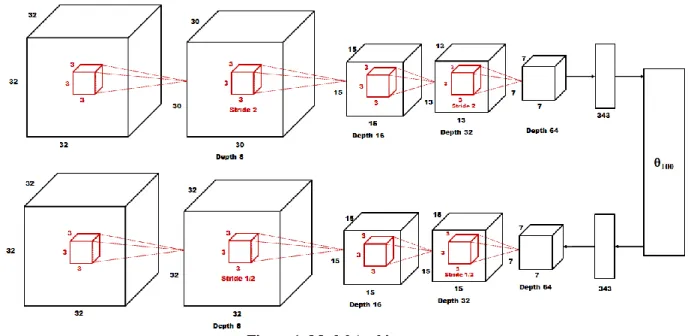
Figure 1: Model Architecture

Model Architecture

The model comprises an encoder network, the latent layer, and a decoder network, as displayed in Figure 1. The encoder network consists of 4 convolutional layers and a fully connected layer, which is itself fully connected to the latent layer. The decoder network has an identical, but inverted, architecture. The network weights are not tied. Each convolutional layer has a bank of 3x3x3 filters, starting with 8 filters in the first layer and doubling at each subsequent layer.

All layers use the exponential linear unit [16] nonlinearity, with the exception of the final layer, which uses a sigmoid nonlinearity. The output of each element of the final layer can be interpreted as the predicted probability that a voxel is present at a given location.

Downsampling in the encoder network is accomplished via strided convolutions (as opposed to pooling) in every second layer. Upsampling in the decoder network is accomplished via fractionally strided convolutions, implemented as the gradient of an equivalent strided convolution, in every second layer[17].

The network is initialized with Glorot Initialization [18], and all but the output layer are Batch Normalized[19]. The variance and mean parameters of the latent layer are individually batch normalized, such that the output of the latent layer during training is still subject to random noise under the VAE parameterization trick.

Loss Function

The loss function consists of the KL divergence prior on the latents, L2 weight regularization, and the reconstruction error, for which we use a specialized form of Binary Cross-Entropy (BCE). The standard BCE loss is:

ℒ = −𝑡 log(𝑜) − (1 − 𝑡) log(1 − 𝑜)

Where t is the target value in {0,1} and o is the output of the network in (0,1) at each output element. The derivative of

approaches t, which results in small gradients that can cause the network to prematurely stop learning during training.

Additionally, the standard BCE weights false positives and false negatives equally. Because ~95% of the voxel grid in the training data is empty, the network tends to confidently plunge into a local optimum of the standard BCE by outputting all negatives.

We make two key modifications to the BCE to improve training. First, we change the range of the target to {-1,2}, increasing the magnitude of the loss gradient throughout the domain of o when t is negative, and reducing the probability of vanishing gradients. Second, we add a hyperparameter γ which weights the relative importance of false positives against false negatives:

ℒ = −𝛾𝑡 log(𝑜) − (1 − 𝛾)(1 − 𝑡) log(1 − 𝑜)

The derivative of the BCE with respect to the output is plotted in Figure 2, for the case of a negative target value and γ=0.5.

During training, we set γ to 0.97, strongly penalizing false negatives while reducing the penalty for false positives. Setting γ too high results in noisy reconstructions, while setting γ too low results in reconstructions which neglect salient object details and structure.

Training

The model is trained using stochastic gradient descent with Nesterov momentum [reference] for 100 epochs, or until the error on a held-out validation set bottoms out. The learning rate is set to 0.0001 for the first epoch, then increased to 0.001 for the remaining 99 epochs. The data is augmented by adding random jitter noise to each training example, as in [12]. A combination of corrupted and uncorrupted data is used as both the input and the target of the system, as opposed to using the uncorrupted data as the target example. By training the network to reconstruct the corrupted data, we force it to learn invariance to small structural variations, and additionally increase

Experiments

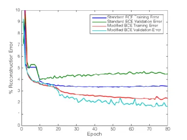
We first validate our modification to the BCE by comparing the validation errors of two identical networks, one trained with the standard BCE, and one trained with our modification. The reconstruction error is plotted against training epochs in Figure 3. Interestingly, we note that the validation error is lower than the training error for this particular training run.

Figure 3: Comparison of Training Regimes

We experiment with a number of different model architectures and training regimes before converging on the final architecture detailed above. In particular, we experiment with augmenting the training objective by adding a 10-unit fully connected softmax layer for classification in parallel with latent estimation, as well as a denoising objective, corrupting the input with random jitter noise and using the uncorrupted input as the reconstruction target. Neither of these changes result in an improvement in performance.

After training for 100 epochs, the model achieves 99.01% mean reconstruction accuracy on the test set. Table 1displays the confusion matrix for the test set.

Table 1: Test Set Reconstruction Confusion Matrix

Test Predicted: Negative Predicted: Positive

Actual: Negative 99.39% 0.61%

Actual: Positive 7.64% 92.36%

5. DISCUSSION

The network achieves passable reconstruction accuracy, and learns to smoothly interpolate between arbitrary, previously unseen shapes. The network is additionally capable of generating random shapes with consistent structure, indicating that the learned latent space is successful in disentangling the factors of structural variation, though these new shapes.

The network performs well for dense objects, particularly thick dense objects such as sofas and toilets, but occasionally struggles to reconstruct objects with long, thin members, such as tables or chairs with thin legs. Presumably, these features are too small to activate in the receptive field of the appropriate latents, and are lost in favor of denser features which weigh more heavily in the loss function.

The network also struggles to reproduce crisp edges, preferring to output smooth, rounded edges. This is analogous to the way in which a 2D autoencoder will tend to output images with blurry edges rather than crisp edges to avoid overconfidently making incorrect predictions.

Interpolation

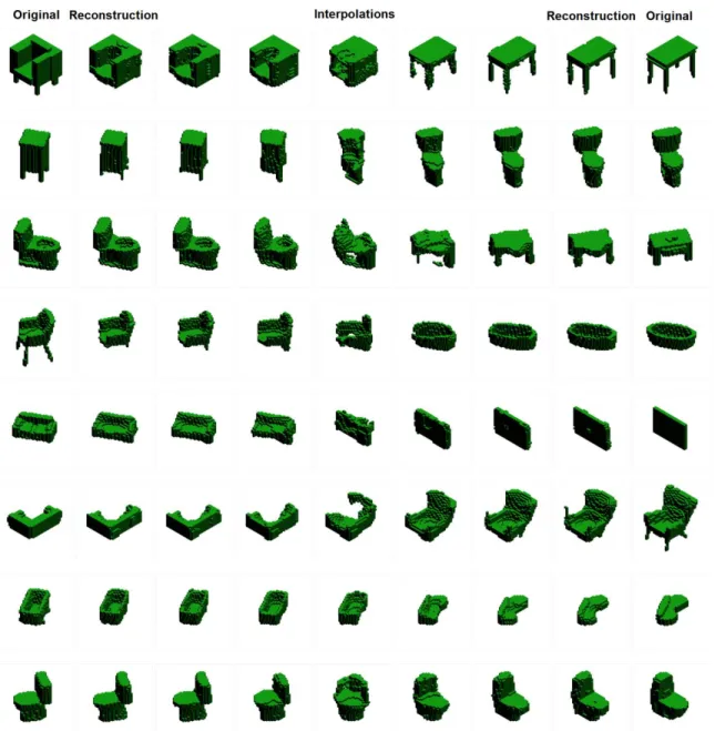
The system is capable of smoothly interpolating between reconstructions, indicating that it learns a representation which captures the underlying factors of structural variation. For example, when interpolating between two objects of the same class but slightly different orientation, the model will make only minimal changes in the output during interpolation, rather than completely deconstructing and reconstructing the output (i.e. passing through zero in the latent space), as can be seen in the last row of Figure 5.

When interpolating between drastically different objects, the interface exhibits a “flowing water” effect, wherein preexisting voxels will appear to smoothly shift between shapes, rather than appearing at random, as can be seen in the first three rows of Figure 5.

Random Object Generation

By sampling a random latent vector from the standard multivariate normal, we generate class-unconditional random objects, shown in Figure 4. These objects consistently bear a semblance of structure, with few to no free-floating voxels, suggesting that the decoder network has learned to maintain output voxel connectivity regardless of the latent configuration.

Figure 4: Randomly Generated Objects

Figure 5: Example Interpolations. The rightmost and left most images are the original objects, the adjacent images are the network’s reconstruction, and the images between show interpolations in the latent space.

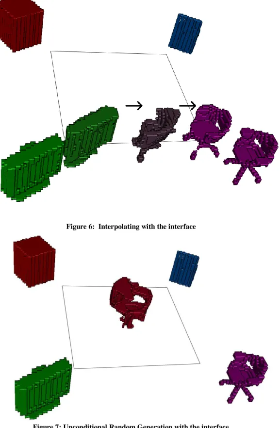
Figure 6: Interpolating with the interface

6. USER INTERFACE

We present a graphical user interface modeled after [7]. The interface, implemented using VTK [15], supports interpolating between up to four different models, as well as class-unconditional random shape generation. The models are randomly selected from the Modelnet test set at runtime, and the entire Modelnet test set can be randomly cycled through by tapping the arrow keys. Figure 6 shows a screenshot of the interface, where the center object is shown while interpolating between a monitor and a chair, and Figure 7 shows unconditional random generation.

When a new set of models is loaded into the interface, the system immediately runs the models through the encoder network to obtain the deterministic latent representation of each model, and stores those latent values in memory. The user may then click and drag the center object between the four interpolant endpoint objects, interpolating linearly between the latent representations of those endpoints. As the user interpolates in the latent space, the decoder network runs inference in real time and outputs the interpolated object. A video of the interface in action is available online [20].

7. LIMITATIONS AND FUTURE WORK

The primary limitation of the system in its current form is its inability to perform class-conditional random object generation. Future work will focus on augmenting the latent space with a class-conditional encoding to permit generation of objects which clearly resemble objects such as chairs and tables. Additionally, future work will experiment with modifications to the network’s loss function to deal with the network’s tendency to neglect certain object features, i.e. by making use of an adaptive γ parameter or perceptual similarity metrics [6].

8. CONCLUSION

We present a method for training and evaluating generative voxel models using 3D convolutional variational autoencoders. Our method works with entirely unlabeled and unsegmented data, and is capable of interpolating between objects of disparate class. We develop an interface that allows users to interactively explore a geometrically coherent latent space. This intuitive interface provides the user with direct control over the content generated, without requiring extensive low-level manipulation of geometric primitives.

ACKNOWLEDGMENT

This research was made possible by grants and support from Renishaw plc and the Edinburgh Centre For Robotics. The work presented herein is also partially funded under the European H2020 Programme BEACONING project, Grant Agreement nr. 687676.

REFERENCES

[1] C. Szegedy, W. Liu, Y. Jia, P. Sermanet, S. Reed, D. Anguelov, D. Erhan, V. Vanhoucke, and A. Rabinovich. Going deeper with convolutions. CVPR, 2015.

[2] A. Radford, L. Metz, and S. Chintala. Unsupervised representation learning with deep convolutional generative adversarial networks. arXiv preprint arXiv:1511.06434, 2015.

[3] A. Dosovitskiy, J.T. Springenberg,and T. Brox. Learning to

generate chairs with convolutional neural networks. arXiv preprint arXiv:1411.5928, 2014

[4] T. Kulkarni, W. Whitney, P. Kohli, Pushmeet, and J. Tenenbaum, Deep convolutional inverse graphics network. In Neural Information Processing Systems, 2015.

[5] D.P. Kingma and J. Ba. Adam: A Method for Stochastic Optimization. arXiv: 1412.6980, December 2014.

[6] A. Lamb, V. Dumoulin, and A. Courville. Discriminative Regularization for Generative Models. arXiv: 1602.03220v4, 2016.

[7] M. Yumer, P. Asente, R. Mech, and L. Kara. Procedural Modeling Using Autoencoder Networks. In Proceedings of the 28th annual ACM Symposium on User Interface Software and Technology, 2015.

[8] E. Kalogerakis, S. Chaudhuri, D. Koller, and V. Koltun. A probabilistic model for component-based shape synthesis. ACM Transactions on Graphics (TOG), 31(4), 55, 2015.

[9] M. Averkiou, V. G. Kim, Y. Zhen, and N. J. Mitra. Shapesynth: Parameterizing model collections for coupled shape exploration and synthesis. Computer Graphics Forum (Eurographics) 33, 2014.

[10] K. Xu, H. Zhang, D. Cohen-Or, and B. Chen. Fit and diverse: set evolution for inspiring 3D shape galleries. ACM Transactions on Graphics (TOG), 31(4), 57, 2012.

[11] Z. Wu, S. Song, A. Khosla, F. Yu, L. Zhang, X. Tang, and J. Xiao, 3D Shapenets: A deep representation for volumetric shape modeling. CVPR, 2015.

[12] D. Maturana and S. Scherer. VoxNet: A 3D Convolutional Neural Network for Real-Time Object Recognition. IEEE/RSJ International Conference on Intelligent Robots and Systems (IROS), 2015.

[13] The Theano Development Team. Theano: A Python framework for fast computation of mathematical expressions. arXiv: 1605.02688, 2016.

[14] Lasagne: A Lightweight Library to Build and Train Neural Networks in Theano. https://github.com/Lasagne/Lasagne [15] W. Schroeder, K. Martin and B. Lorenson. The Visualization Toolkit, 4th edition. Kitware, ISBN 978-1-930934-19-1. 2006.

[16] D. Clevert et al. Fast and Accurate Deep Network Learning by Exponential Linear Units (ELUs). arXiv: 1511.07289, 2015.

[17]. V. Dumoulin and F. Visin. A guide to convolution arithmetic for deep learning. arXiv preprint, arXiv: 1603.07285. 2016.

[18] X. Glorot and Y. Bengio. Understanding the Difficulty of Training Deep Feedforward Neural Networks. In Proc. AISTATS, 2010, pp. 249–256.

[19] S. Ioffe and C. Szegedy. Batch Normalization: Accelerating Deep Network Training by Reducing Internal Covariate Shift. arXiv:1502.03167, 2015.