Does the regulation of manure land application work
against agglomeration economies?
Theory and evidence from the French hog sector
Carl GAIGNÉ, Julie LE GALLO, Solène LARUE, Bertrand SCHMITT
Working Paper SMART – LERECO N°11-02
August 2011
UMR INRA-Agrocampus Ouest SMART (Structures et Marchés Agricoles, Ressources et Territoires) UR INRA LERECO (Laboratoires d’Etudes et de Recherches Economiques)
Does the regulation of manure land application work against agglomeration
economies?
Theory and evidence from the French hog sector
Carl GAIGNÉ
INRA, UMR1302, F-35000 Rennes, France Agrocampus Ouest, UMR1302, F-35000 Rennes, France
Julie LE GALLO
CRESE, Université de Franche-Comté, F-25000 Besançon, France
Solène LARUE
INRA, UMR1041 CESAER, F-21000 Dijon, France Bertrand SCHMITT
INRA, UMR1041 CESAER, F-21000 Dijon, France
Auteur pour la correspondance / Corresponding author Carl GAIGNÉ
INRA, UMR SMART
4 allée Adolphe Bobierre, CS 61103 35011 Rennes cedex, France
Email: Carl.Gaigne@rennes.inra.fr Téléphone / Phone: +33 (0)2 23 48 56 08 Fax: +33 (0)2 23 48 53 80
Does the regulation of manure land application work against agglomeration economies? Theory and evidence from the French hog sector
Abstract
The well-known increase in the geographical concentration of hog production suggests the presence of agglomeration economies related to spatial spillovers and inter-dependencies among industries. In this paper, we examine whether the restrictions on land application of manure may weaken productivity gains arising from the agglomeration process. We develop a model of production showing the ambiguous spatial effect of land availability and the restriction on the manure application rate. Indeed, while the regulation of manure application triggers dispersion when manure is applied to land as a crop nutrient, it also prompts farmer to adopt manure treatment that favors agglomeration of hog production. Estimations of a reduced form of the spatial model with a spatial HAC procedure applied to data for French hog production for 1988 and 2000 confirm the ambiguous effect of land limitations induced by the restrictions on manure application. It does not prevent spatial concentration of hog production, and even boosts the role played by spatial spillovers in the agglomeration process.
Keywords: hog production; land availability; manure application regulation; agglomeration
economies; spatial econometrics.
La réglementation de l’épandage du lisier va-t-elle à l’encontre des économies d’agglomération ? Théorie et application au cas de l’élevage porcin en France
Résumé
L'augmentation de la concentration géographique de la production porcine suggère la présence d'économies d'agglomération liées aux externalités spatiales et des interdépendances entre les industries. Dans cet article, nous examinons si les restrictions à l'épandage du lisier (directive nitrate) peut affaiblir les gains de productivité découlant du processus d'agglomération. Nous développons un modèle spatial de production montrant l'effet ambigu de la disponibilité des terres et de la restriction sur le taux d’application du lisier. En effet, si d’un côté, la directive nitrate favorise la dispersion lorsque le lisier est épandu comme un élément nutritif des cultures, elle incite également les agriculteurs à adopter des technologies de traitement du lisier qui favorise l'agglomération de la production porcine. Les estimations d'une forme réduite du modèle spatial à l’aide d’une procédure HAC spatiale appliquée aux données de la production porcine française de 1988 et 2000 confirment l'effet ambigu de la directive nitrate concernant les restrictions sur l'épandage de lisier. Toute chose égale par ailleurs, cette restriction ne fait pas obstacle à la concentration spatiale de la production porcine, et renforce encore le rôle joué par les externalités spatiales dans le processus d'agglomération.
Mots-clefs : production porcine, disponibilité des terres, directive nitrate; économies
d'agglomération; économétrie spatiale.
Does the regulation of manure land application work against agglomeration economies? Theory and evidence from the French hog sector
1. Introduction
Empirical evidence suggests that the spatial concentration of hog production promotes a rise in hog farm productivity. For the United States, Key and McBride (2007) report that, between 1992 and 1998, hog production shifted from the Heartland to the Southeast, and mean farm output increased much more in the Southeast (see also Abdalla et al., 1995). The findings are
similar for Europe. For example, in France, Brittany is hosting an increasing share of hog production and the productivity in this region has improved (Daucé and Léon, 2003). It appears that agglomeration can be a source of productivity gains in hog rearing (Roe et al.,
2002).
However, spatial concentration of hog production is a serious source of water course (rivers and streams) pollution. In many countries (France, Denmark, the Netherlands, the United States), spatial concentrations of animal production units on limited land areas have exceeded the public authority manure management regulations. In the European Union (EU) the Nitrates Directive, and in the United States (US) the Clean Water Act were introduced to protect bodies of water from pollution by nitrates from agricultural sources. In the EU, manure applications are limited to a maximum level of nitrogen per hectare and per year. This restriction on manure spreading creates difficulties for regions with high livestock densities: there is simply not enough land available to accommodate the amounts of manure being produced. The stringency of the EU Nitrates Directive and the non-negligible costs of compliance are having the effect of some hog producers exiting the sector or scaling down their hog and manure production.
In this context, this paper studies the effect of land availability on the location of hog production and agglomeration economies. Because there is a restriction on the application of animal manure to land, land limitations are expected to reduce the spatial concentration of production and, in turn, to affect the productivity gains related to agglomeration economies. However, the situation is not so clear cut, and is deserving closer attention. Farmers can adopt two types of manure management: (i) spreading the animal manure on land as a crop nutrient or/and (ii) treating the manure in order to reduce the nitrogen content, and also its odor and volume. In the first case, increasing hog production implies that the farmer will have to spread
the resulting larger volumes of manure on more and more distant cropland. Because hauling crop nutrients in the form of manure is relatively expensive, the cost of this type of manure management increases not only with the increase in hog production but also with the distance to the cropland. This creates incentives for producers located in areas with higher hog density to reduce their production. In this case, manure spreading triggers the dispersion of hog production. In the second case, manure treatment technology aims at reducing the volume (so that manure and nutrient transport costs become negligible) and improving market prospects by changing the nutrient composition. However, there are substantial fixed costs attached to this practice (IFIP, 2002) with the result that this manure management technology may favor agglomeration of hog production. Because manure treatment technology exhibits economies of scale, this system of management is more profitable at high levels of hog production. In other words, the use of treatment technology at either the individual or the collective level promotes agglomeration. As a result, the regulation on manure application could trigger dispersion or agglomeration of hog production depending on the type of manure management system chosen by the farmer.
To determine how land limitations induced by the regulation on manure application in the EU affect the location of hog production and agglomeration economies in the hog sector, we first develop a model of location and production in which farmers can choose among different technologies to manage manure. Next, we test the main predictions of our framework using French data. We control for other factors that shape the spatial structure of hog production. More precisely, we identify agglomeration economies by distinguishing market and non-market forces.
Cronon (1991) in his famous book, Nature’s Metropolis, provides a detailed description of the
market factors explaining the process of agglomeration related to hog production in Chicago and its hinterland, that occurred in the second half of the 19th century (see the chapter entitled
Porkopolis). First, the proximity between the farmers and the slaughterhouses may be a key
determinant. As Cronon (1991) notes, the incentives to slaughter and pack pigs near to where they were raised are strong. Transporting the animals is expensive in terms of relatively high transport costs and the loss of weight suffered by the hogs during the journey. Cronon showed that it was unprofitable, therefore, to transport them over long distances. A second factor explaining the local growth of hog production is geographic proximity between hog producers
and crop producers (or feed suppliers).1 Both factors induce large productivity gains, which, combined with innovations in meat transportation to serve final consumers and increased productivity of pork packers, enabled Chicago and its surrounding area to produce and pack very large quantities of hog meat (in the 1870s, over a million hogs were slaughtered annually in Chicago). Although Cronon’s explanations are related to the relative transport costs and scale economies observed around Chicago in the second half of the 19th century, these arguments should still hold as an explanation for the agglomeration of hog producers in a few locations. Indeed, the ratio of transport costs to output or input prices in the pork sector is far from negligible. New economic geography provides rigorous frameworks to explain the role of increasing returns and trade costs in agglomeration processes (Fujita and Thisse, 2002). The literature shows that producers can benefit also from geographical proximity to other producers in the same sector: non-market interactions or so-called “Marshallian externalities” act as a shift factor that modifies the relationship between cost and output. Geographical proximity induces more personal interaction and contacts, which, in turn, facilitate the transmission of information regarding changes in output and input markets as well as the development of technical or organizational innovations or new inputs (Duranton and Puga, 2004), or information spillovers. Frequent contacts among others in the sector also allow
purchasers and suppliers to build the trust required to write incomplete contracts as shown in Leamer and Storper (2001). In other words, the productive efficiency of farmers should increase with the number of farms established in the same area, and decrease with an increase in the distance between them.
Our study differs sharply from recent empirical work on the role of traditional location factors and environmental regulation in the location of animal production. First, the focus on the impact of the stringency of environmental regulation on the location of animal production has not been matched by an equal attention to the impact of the regulation on manure application and its implication in terms of land availability on the process of agglomeration. For example, Metcalfe (2000, 2001), Isik (2004) and Roe et al. (2002) study how differences in the
stringency of environmental regulations among US States affect the location of animal production but they do not test the role of land availability induced by the regulation on manure application rate in the agglomeration of hog production. Second, we build a
1 As pointed out by Cronon (1991, p. 226): “
Their prodigious meat-packing powers meant that once farmers had harvested their corn crop, pigs (along with whisky) were generally the most compact and valuable way of bringing it to market”.
theoretical model that allows us to identify the relationship between location and hog production when manure application rates are restricted and farmers can choose different technologies to manage manure. The combined effects of spatial spillovers, access to suppliers or purchasers, manure application regulation and negative externalities on local production are not a priori obvious and can lead to serious problems related to identifying and
evaluating the respective roles of these different factors. Thirdly, we implement recent developments in spatial econometrics to take account of some crucial biases that have so far been ignored. The approach in Roe et al. (2002) does not control for the endogeneity of the
location of slaughter facilities or input suppliers, while hog production and production of other livestock by hog producers are determined simultaneously in different areas. In addition, unlike Isik (2004) who uses stage least squares, we perform a generalized spatial two-stage least squares estimation (GS2SLS), as suggested by Kelejian and Prucha (1998), combined with a heteroskedastic and autocorrelation consistent non-parametric estimation of the variance-covariance matrix (Kelejian and Prucha, 2007) to control for un-modeled factors in the residual terms.2
Our theoretical model shows that the regulation on land application of manure has an ambiguous effect on the spatial distribution of hog production. By favoring the use of a manure treatment system, stricter regulation on manure application rates or a decrease in the land available for manure application might trigger the spatial concentration of hog manure. Furthermore, our framework shows that a larger share of manure managed by treatment technology strengthens the role of agglomeration economies in the form of productivity gains. Our empirical tests of these predictions confirm the ambiguous effect of the ratio of manure production to available land on hog production. In accordance with our theoretical model, an increasing ratio of local manure production to land availability increases the density of hog production while a rise in this ratio for the surrounding counties triggers dispersion. The total effect is more likely to be negative but not significant. In other words, land limitations induced by the regulation on manure application do not seem to work against the spatial concentration of hog production. In addition, our results suggest that the regulation on manure application rates has boosted the role played by non-market spatial externalities in the agglomeration process.
2 This method is also used in Ben Arfa
et al. (2010) and Abiltrup et al. (2010) to explain the spatial structure of
The rest of the paper is organized as follows. In the next section, we develop the theoretical model; in the third section, we present the empirical model and discuss econometrics issues. The fourth and fifth sections present the data and report the results; they are followed by a concluding section.
2. Theory
We develop a spatial model of hog production to clarify the impact of manure application regulation on the hog producer’s choice according to her/his location. The model takes account of spillovers, linkages to feed suppliers and slaughter facilities/processors, and manure management.
General framework
Consider an economy with R regions, labeled r=1,...,R separated by a given physical
distance and with three types of producers (hog producers, slaughterhouses and feed producers). Each region is formally described by a one-dimensional space y. Each region
hosts one slaughter facility (SF) located at the origin y=0, I farms located at yi with
(or at distance 1,...,
i= I yi from the SF) surrounding the SF. The density of farms at each
location is equal to 1 (as long as the profits of farms are non null). There are K feed producers
located at yk with k=1,...,K. The distance between farmer i and feed producer k is given by
ik k i
u ≡ y −y . We focus on the behavior of a farmer producing in location i and belonging to
region r. Because in our framework there are no interactions between hog or input producers
located in different regions, in our notations we can drop the index (r) identifying the region
where the farmer produces (we consider only the impact of final consumers’ location on production). We assume that the profit function of a hog producer is given by:
( )
( ) . i zr y hi i C g
π = −τ − − (.) (1)
where is the unit price of pork prevailing in region zr r (each farmer is a price taker), τ is the
unit cost of transporting the pigs between farms and the slaughter facility, is the production level of farm i, is the cost function in producing output and is the cost function in
manure management. Implementation of environmental regulations implies compliance costs i
h
(.)
for producers thereby reducing profits. We assume that the cost function is additively separable into output and manure management.
The technology of production is given by hi =A f xi ( )k where xk is the quantity of inputs used
by farms with fx >0 and fxx <03
i j
so that the marginal productivity of each production factor decreases. Note that A =
∑
aij where represents information spillovers received by a farmer located atij
a
i
y from a farmer located at . Hence, represents the information field,
which is a spatial externality. The amount of information received by a farm depends on the mass of farms (equal to 1 in our model) and on its location relative to the others. We consider:
j
y Ai
ij j i
a =ρ y −y −δ (2)
where 0ρ > and δ >0 are two positive constants, δ measuring the intensity of the distance-decay effect and ρ being a scale parameter. There is a large literature related to agglomeration economics on these types of technological externalities, which, in modeling terms, have the additional advantage of being compatible with the competition paradigm (see Fujita and Thisse, 2002, chapter 6).
Given the technology of production, the cost function depends positively on and negatively on with , (.) C 2 h i h i A Ch ≡ ∂C/∂ >hi 0 Chh ≡ ∂2C/∂ >i 0 and ChA≡ ∂2C/(∂ ∂hi Ai)<0, as
well as on the wage rate (denoted w) and the cost of feed (or crop when the feed is produced
by the hog farmer) incurred by the farmer (denoted ηik). We assume that ηik =η ξk+ kuik
where ξk is the unit transport cost of feed between farms and feed producers (uik is the distance between the two) and ηk is the feed producer’s price. Thus, we consider that the farmer incurs transport costs for each type of feed (or crop) input.
Next, we take into account the fact that manure management is regulated. Environmental regulation not only implies compliance costs for producers but also that manure application rates cannot exceed a threshold value. Hence, we consider that one unit of available cropland cannot exceed m units of manure and that s units of cropland are available at each location i.
3 fx denotes the first derivative of
f(.) with respect to each component. The second derivative is subsequently
Let θ be the quantity of manure for each unit of output so that θhi is the quantity of manure
that farmer i has to manage. Note that, in our framework, manure is regarded as a waste
material for the hog producer.4 Farmer i may use two types of manure management
technology: spreading or/and treatment. Farmer i allocates a fraction μi of manure to
spreading.5 Each farmer can also use a manure treatment facility with a capacity (1 μ θ) = − i v ,, 2 2 1 1/ i c c ∂ <v i ≡ ∂ i h 0 0
and a cost function characterized by , , and . What matters for our study is the fact that treatment technology is characterized by an average cost decreasing with the quantity of treated manure (IFIP, 2002) and that the cost of transporting treated manure is not significant. If the farmer chooses to spread manure, he/she incurs the costs of application given by where
1( )i c v c1' ≡ ∂c1/∂ >vi 0 2( )i c m 3 3 1/ i c v ∂ ∂ = μ θi hi = i
m and with c'2 ≡ ∂c2/∂ >mi 0 and ∂2 2/∂ i2 =0
) (
g ≡c v +
c m
(.
. Without loss of generality, we assume that the technology for applying manure yields constant economies of scale. Hence, the costs associated with manure management including the costs of treatment, manure application and manure transport are given by 1 ) 2( ) where
m j m j y y τ − +
∫
m s yij d m i c mi my τis the unit transport cost (including travel time) between where the manure is stored and the field where the manure is spread,6 and mij is the mass of manure applied in location j on a unit
of cropland by farmer i. Given our assumptions, each farmer applies the same quantity of
manure at each location (mij =m).7 Each farmer has ni places around his/her farm where the
manure can be applied, with ni =μ θi h mi/
s. Hence, the total transport cost related to manure 4
Manure is now largely a disposal problem and more land is needed to properly dispose of animal wastes (Keplinger and Hauck, 2006). Indeed, increasing livestock densities reduce manure value and transform this potential resource into a waste whose disposal is costly. In addition, some empirical studies suggest that organic manure demand is relatively low (Feinerman and Komen, 2005).
5 Innes (2000) provides a detailed analysis of the spatial impact of environmental regulation on livestock
production with respect to the location of producers. However, this author does not analyze restrictions on manure application per unit of land and considers hog production as given. Kaplan et al. (2004) provide an
analysis of economic and environmental implications when land application of manure is restricted but they do not consider the spatial effects.
6 Transporting manure is time consuming (and increases with the distance travelled). 7 Except for the more distant location where 0≤ ≤
ij
m m. For the sake of simplicity, we assume that farmers spread the same quantity of manure at each location.
spreading incurred by a farmer is equal to /2
0 2 ni
myms yd τ
∫
. In addition, we assume that ,, 1 c isnot so high that there are no increasing returns to scale in overall production (Chh+ghh >0). Hence, the cost function of manure management can be rewritten as follows:
2 2 2 1 2 (.) ( ) ( ) 2 μ θ τ = + + i i i i m h g c v c m ms (3)
Knowing that vi = −(1 μ θi) hi and mi =μ θi hi, the marginal cost of manure management (gh ≡ ∂ ∂g/ hi) is given by: ' ' 2 2 1 2 (1 μ θ) μ θ τ μ θ / 0 = − + + > h i i m i i g c c h ms (4)
The marginal cost increases with the quantity of manure per unit of output θ, more restricted application rates (lower m), lower availability of surrounding cropland (low s)and cost of
transport between the farm and the manured field τm whereas the marginal cost varies with hog production as follows:
2 ,, 2 2 2 1
(1 ) /
hh i m i
g = −μ cθ +τ μ θ ms (5)
which can be positive or negative. It appears that manure spreading yields decreasing economies of scale because of manure transport costs.
Restrictions on manure application rate, location and production
The equilibrium output ( ) for each farm is implicitly defined in the following equality: *
i h * ( r i) h( , , )ik i i h( , , , , , )i m i i z y C A h g m s h h * 0 π τ η θ μ τ ∂ = − − − = ∂ (6)
We first analyze the direct effect of the restriction on manure application and land availability on production (at a given value of μi). By using (6) and the envelope theorem, we have
*
/ ( ) ( ) / ( s) 0=
h hh hh i
g ms C g h m
−∂ ∂ − + ∂ ∂ , and knowing (4), we obtain:
* / ( ) 2 2 / ( ) 0 ( ) i h m i i hh hh hh hh h g ms h ms ms C g C g τ μ θ ∂ −∂ ∂ = = ∂ + + 2 > (7)
Remember that . It appears that stricter regulation on manure application rates (low
0 hh hh
C +g >
magnitude of this effect increases with . In other words, stricter regulation on manure application rates or lower availability of surrounding cropland works against agglomeration of hog production because of the increasing cost of spreading manure.
i h
However, in (7), we assume that μi does not react to a change in the application rate (m) or in land availability (s). When μi is endogenous, the effect of ms becomes ambiguous.
Indeed, each farmer chooses μi in order to minimize the cost of manure management (3), for a given hog production. Hence the equilibrium share of manure managed by spreading μ*
i minimizing g(.) is implicitly given by ∂g(.) /∂ =μi 0. By plugging vi = −(1 μ θi) hi and
μ θ = i i
m hi into (3), ∂g(.) /∂μi =0 is equivalent to:
' ' 1( )i c2( i) m i i 0 h c v m ms μ θ τ − + + = (8) where μ*
i is an interior solution when
2 (.)/ μ2 0
∂ g ∂ i > or, equivalently, ,, 1 m/
c +τ ms>0 (see
Appendix A.1 for more details). In Appendix A.1, we show that:
* 2 2 2 d 0 d i i i i i g g h h μ μ μ ∂ ∂ = − < ∂ ∂ ∂ and * 2 2 2 d 0 ( ) d( ) i i i g g ms ms μ μ μ ∂ ∂ = − > ∂ ∂ ∂ ,
as long as . In other words, manure treatment technology is more likely to be used when hog production is relatively high and when the manure application rate is strictly limited. Hence, when
*
1>μi >0
μi is endogenous, equation (7) becomes:
* 1 d * ( ) ( ) d( ) i h h hh i i h g g ms C ms ms μ μ − + ⎛ ⎞ ∂ − ⎜ ∂ +∂ × ⎟ ⎜ ⎟ ∂ + ⎜∂ ∂ ⎟ ⎝ ⎠ hh g = (9)
where we have now:
* d d h h i hh i i g g g g h h μ μ hhi ∂ ∂ × <∂ = + ∂ ∂ ∂ 0 (10) where ∂gh/∂ >μi as long as (see Appendix A.2). The detailed expression of (9) is
given in Appendix A.3. As a result, stricter manure application regulation or decreasing land availability has an ambiguous effect on hog production. Even though the direct effect works against agglomeration of hog production (because of the costs associated with manure spreading), the indirect effect favors hog production because the use of treatment technology
*
increases. Hence increasing the capacity to treat manure may promote economies of scale in manure management that offset additional costs of compliance.
We now study the impact of location on hog production for a farmer located at i. In addition,
at a given distance from the slaughter facility, the impact of the distance to a feed producer on hog production is as follows:
* / 0 i h ik k ik hh hh h C u C gη ξ ∂ ∂ ∂ = < ∂ + (11)
As expected, increasing distance to an input supplier reduces hog production. It also appears that the magnitude of the effect of distance increases when manure application is strictly limited and land availability declines. Indeed, by using (5), we show in Appendix A.4 that:
* d d 0 d d hh hh hh i i g g g ms ms ms μ μ ∂ ∂ = + > ∂ ∂ (12)
Hence, the restrictions on the manure application rate favoring the adoption of manure treatment technology induce more hog production around input producers.
Further, it appears that the magnitude of the effect of proximity to a feed producer on hog production increases with the weight of this input in the production process (because
/ h
C ηik
∂ ∂ increases). Hence, we expect that a farm’s hog production is strongly affected by its accessibility to feed suppliers because the expenditure on feed represents more than 50 percent of the hog producer’s production costs.
Concerning the impact of the distance to the slaughter facility on farm i’s production, the
relationship is more complex. Indeed, at a given distance to the input suppliers, we have:
* 0 τ ∂ − = − + < ∂ + + ∂ i hA i hh hh hh hh i h C y C g C g y ∂Ai (13) The first term on the RHS in (13) concerns unit cost of transporting the hogs between farm and the SF; the second term on the RHS captures the influence of a change in location on the intensity of spillovers. Without information spillovers, hog production decreases with respect to the distance from the SF. The slope increases with the cost of transporting hog units (τ ) and with the share of manure managed by a treatment system ( decreases). When information spillovers occur, we have
hh
g
/
i i
A y 0
the distance to the SF is higher in the presence of technological externalities. As mentioned above, decreasing land availability makes the slope steeper.
We next turn to the impact of a consumption shock on hog production. More precisely, we study the impact of a shock in the demand prevailing in region r’. We know that the regional
price of pork depends positively on the demand for pork and thus on the spatial distribution of consumers, because transport costs increase consumer prices. We denote the demand for pork by consumers located in region r’ from producers located in region r by where
is the transport cost, increasing with the distance between the region where the pork is produced and the region where the pork is consumed, whereas
' ( ' , )' r r r r r D t I ' r r t ' r
I is the income in region r’.
Because and (the total demand addressed to producers in region r),
some standard calculations reveal that:
' ( r r z I ) Dr = Σr'Dr r' (dr r' ) * ' ' ( ) 0 i r r r r hh hh r h d t z I C g D ∂ = ∂ > ∂ + ∂ (14)
with which is decreasing with interregional transport cost. Hence, the impact of a change in the wealth prevailing in a region depends both on the transport costs of the processed product and on the relationship between the regional pork price and regional demand
', ' '
(r r) r / r
d t = ∂D ∂I
To sum up, our model shows that the restrictions on land application of manure and land availability have an ambiguous effect on the spatial distribution of hog production. On the one side, the regulation on manure application rates triggers dispersion when manure is applied to land as a crop nutrient. On the other side, by favoring the use of treatment systems, stricter restrictions on manure application rates or a decrease in land available for manure spreading trigger the spatial concentration of hog manure. Furthermore, low land availability and a low limit value of the manure application rate strengthen the agglomeration economies related to information spillovers and access to slaughter facilities and to input suppliers.
3. Empirical model, data and econometric issues Empirical model
Given the discussion in the previous section, we aim at evaluating the impact of land availability for manure spreading on the spatial re-allocation of hog production and, in turn, to evaluate to what extent restrictions on the manure application rate affect agglomeration economies. To test our theoretical predictions, we consider the following empirical model, which is a spatial lag model:
h
H=ρW H+γMΜ+ XγX +γZZ+ε (15)
where is a vector containing the observations of the dependent variable (hog production density) in each of the n counties for a given period,
H n×1
ρ is the scalar spatial autoregressive parameter, Wh is an (n n× ) spatial weights matrix. In addition, , , and are , and matrices of
Μ X Z
1 k
n× n×k2 n×k3 k = + +k1 k2 k3 explanatory variables respectively
related to land availability to manure spreading (M), local and neighboring characteristics such as access to markets (X), and additional variables used to test the robustness of our results (Z), whereas ε is a vector of error terms, the properties of which are detailed below. Finally
1 × n M
γ , γX and γZ are the k1×1, k2×1 and k3×1 vectors of unknown parameters
to be estimated. We next describe our database and variables.
Data and variables
The data in this paper are mainly from agricultural (1988 and 2000, before and after the implementation of Nitrates Directive in the EU) and population (1990 and 1999) censuses in France, and the French Pork Sector Institute (IFIP). The spatial unit is the French “canton”
(an administrative delineation similar to a US county). This is quite a fine spatial disaggregation for analysis. Since some units changed during our study period as a result of administrative changes (they merged or split), our analysis is performed on 3,589 units for 1988 and 3,572 units for 2000.
As our dependent variable, because of the heterogeneous sizes of canton, we use the density
of pigs in the county, i.e. the number of hogs per hectare at the canton level expressed in
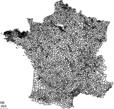
Hog production is quite unevenly distributed across French cantons, with a strong
geographical concentration in some areas, notably Brittany in the West of France.
Figure 1: Geographical distribution of hog density at the county level in 2000.
0 - 12.178 12.178 - 45.596 45.596 - 104.829 104.829 - 190.513 190.513 - 362.627
We list the four broad categories of explanatory variables included in our model. In each case and in relation to our theoretical results, we indicate whether they are considered either exogenous or endogenous. We also detail the instruments used to control for the endogenous variables.
First, the spatial lag of the dependent variable is introduced in order to capture the role of spatial information spillovers in hog production. This variable is denoted , where h is a spatial weight matrix. More precisely, it contains element ij
h
W H W
ϕ as a distance decay function, with (where dij is the physical distance at crow flight in kilometers between the
capital of counties i and j) if the distance is less than 200 km, otherwise 1
ij dij ϕ = −
ij
elements along the main diagonal are ϕij =0. The weights have been standardized so that the elements in each row sum to 1: s
ij ij j ij
ϕ =ϕ
∑
ϕ . Note that ϕij can be interpreted as the role of distance in the decreasing intensity of positive interactions between farmers located in canton i and those located in j (respectively, in the rows and columns of the matrix). The cut-offvalue of 200 km was chosen because it appears that cooperatives (producer organizations via
which information mainly spreads) have a regional field of action. This variable is obviously
endogenous since it is always correlated with error terms, irrespective of the distribution of
the latter (Anselin, 2006).
Second, to capture the role of land limitations in manure spreading (vector Μ) – the variables
m and s in our framework, we build Ni/Li the ratio of the quantity of nitrogen included in
manure produced by all livestock (pigs and other animals) located in cantoni (Ni) to the area
of land available for manure spreading ( ) in order to capture the impact of Li ms. Note that the
land potentially available for manure spreading ( ) represents in France around 70% of the total cultivated area. Because the land available could be in nearby counties, we introduce a spatial dimension of this variable by using the ratio (
i
L
/ j j
N L ) in neighboring places with j≠i,
i.e. the ratio of neighboring places weighted by distance L×( / )
j
j
W N L , where is the
spatial weight matrix related to L/N, in order to capture the transport costs related to manure
spreading (
L W
m
τ in the model). The spatial weight matrix WLcontains elements ϕij with if the distance is less than 100 km, otherwise
1
ij dij ϕ = −
ij
ϕ is set to 0. Hence, in accordance with our model, we consider that land availability for spreading hog manure decreases with livestock production and with the distance between farms and cropland. Ni/Li and its spatial
lag are considered to be endogenous because they include manure produced by hog
production at countylevel.
Third, in order to capture the role of local and neighboring characteristics (vector ), we include accesses to input suppliers, to slaughter facilities, and to final consumers as well as the local degree of urbanization. More precisely, we consider the following four variables:
X
(i) Access to feed producers: we introduce the regional mixed feed production specific to hogs (Mixed Feed). Unfortunately, we were unable to collect precise data on the location and
production of suppliers of industrial mixed feed at the canton level. The available data relate
(ii) Access to slaughter facilities from location i: this variable is noted where
is a vector containing the size of the slaughter facilities at the canton level, is a spatial
weight matrix related to S and I the identity matrix. Therefore, line i in is the size of the
slaughter facility located in canton i plus a distance-weighted average of i's neighboring
facilities. The introduction of the (Ws + I) matrix is aimed at capturing the role of the cost of
transporting alive pigs between the farm and the nearby slaughterhouse. We use the inverse distance matrix. As our cut-off, we consider the minimum distance ensuring that each observation has at least one neighbor. Thus, for , the cut-off is around 34 kilometers. We assume that is endogenous. Indeed, the location of meat processors and hog
suppliers is co-determined by the spatial distribution of hog producers due to market mechanisms or the vertical coordination prevailing in the hog sector.
* ( s S = W +I s W * S )S S S s W * ( ) s S = W +I
(iii) Access to final consumers from location i: this is proxied by the spatial lag of population
( ) where Pop is the population of the canton and is the spatial weight
matrix related to Pop, in order to capture the transport costs of pork to final consumers. is
the inverse distance matrix with a cut-off set to the same distance as the distance to the slaughterhouse. * R Pop =W ×Pop WR R W
(iv) The local degree of urbanization: this is proxied by the population living in the canton
(Pop). This variable captures not only the competition for land with the population but also
the effects of some local manure management regulations. Because hog production induces odors and other ambient effects, regulation on hog production expansion is stricter in urbanized areas. In other words, it is more costly to increase hog production in more populated areas. This constraint (on the producer) creates some additional costs by shrinking the expansion of hog production. Hence, at given land prices, hog production is less likely to
increase in most populated areas. For those reasons, we expect a negative relationship between hog production and the size of the local population (Pop).
Finally, we consider three types of variables (vector Z) in order to test the robustness of our results:
(i) First, we use access to crops (corn and other cereals). This variable captures two effects. On the one hand, crops could be used as inputs (feed for pigs) so that the proximity to crops incites to increase local hog production. On the other hand, it is possible for farmers faced with a nitrogen limitation to switch to a more intensive crop that entails higher manure
nitrogen utilization per hectare.8 We then introduce access to corn and access to other crops:
* ( )
c X c
X = W +I X with Xc, a vector containing the available quantity of crops(corn and other crops). We also consider total nitrogen uptake of crops (as in Kaplan et al., 2004), at the canton level and surrounding cantons ((WX+I)Nuptake). This variable is computed by
multiplying total crop production by nitrogen uptake per unit of crop output and then summing across all crops for each canton. Whatever the mean of cropland, we expect a
positive effect of access to crops. These different measures of access to crops are treated as
endogenous.
(ii) Next we consider the structure of farms. Hog producers fall into three categories based on their different production technologies: farrow-to-finish farms, farrow-to-feeder farms, and feeder-to-finish farms, respectively farmers who breed sows to produce small weanling hogs, farmers who wean and fatten weanlings, and farmers who breed and fatten. The majority of French hog farms are farrow-to-finish farms, so we use the ratio of farrow-to-finish farms to hog farms (FFF share). This variable controls for the effect of production orientation on the
agglomeration of production
(iii) Finally, we include share of non-hog farms in canton i (NHF share) as a control variable
in order to test whether inter-industry economies of scale externalities exist between the different types of animal production, as suggested by Roe et al. (2002). Indeed, hog producers
may benefit from proximity to different livestock producers because they share the same infrastructures, feed suppliers or meat processors, regardless of their industry affiliation. This variable is exogenous.
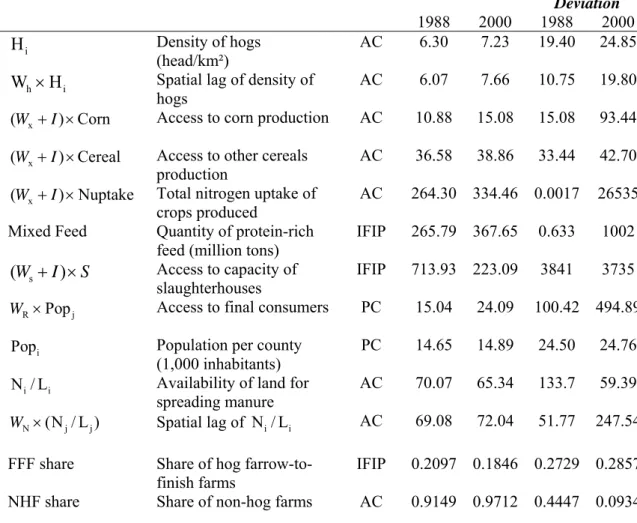
All the variables used to estimate equation (15) are described in Table 1 which presents the definition of each variable, its source and main descriptive statistics.
8 According to the EU nitrate directive, the application of manure is limited to a maximum level of nitrogen from
animal manure per hectare and per year (170 kg N/ha). However, this directive allows for derogation where the threshold value of application rate can be relaxed in the presence of crops with high nitrogen requirements.
Table 1: Description of variables
Variable Definition Source Mean Standard Deviation 1988 2000 1988 2000 i H Density of hogs (head/km²) AC 6.30 7.23 19.40 24.85 h i
W ×H Spatial lag of density of hogs AC 6.07 7.66 10.75 19.80 x (W + ×I) Corn ke j
Access to corn production AC 10.88 15.08 15.08 93.44
x
(W + ×I) Cereal Access to other cereals production
AC 36.58 38.86 33.44 42.70
x
(W + ×I) Nupta Total nitrogen uptake of crops produced
AC 264.30 334.46 0.0017 26535 Mixed Feed Quantity of protein-rich
feed (million tons)
IFIP 265.79 367.65 0.633 1002 s (W + ×I) S Access to capacity of slaughterhouses IFIP 713.93 223.09 3841 3735 R Popj
W × Access to final consumers PC 15.04 24.09 100.42 494.89
i
Pop Population per county (1,000 inhabitants)
PC 14.65 14.89 24.50 24.76
i i
N / L Availability of land for spreading manure
AC 70.07 65.34 133.7 59.39
N (N / L )j
W × Spatial lag of N / Li i AC 69.08 72.04 51.77 247.54
FFF share Share of hog farrow-to-finish farms
IFIP 0.2097 0.1846 0.2729 0.2857 NHF share Share of non-hog farms AC 0.9149 0.9712 0.4447 0.0934
AC: Agricultural census; PC: Population census ; IFIP: French Institute of the Pork Sector.
Econometric issues
To estimate the spatial lag model (15), we use spatial econometric techniques (Anselin, 2006; LeSage and Pace, 2008) and take into account several endogeneity problems. Maximum likelihood (ML) estimation is the most common methodological framework applied in spatial econometrics for such cases since it allows the endogeneity of the spatially lagged variable to be controlled for (Anselin, 2006). This is the approach used by Roe et al. (2002) to
reveal agglomeration economies in the US hog production. However, as argued above, other explanatory variables, such as the location of slaughter facilities or input suppliers, are co-determined with the dependent variable. Although endogeneity can be a source of econometric bias, this problem has been ignored so far. It causes additional econometric complexities, since, as pointed out by Fingleton and Le Gallo (2008), the estimation of such a
h W H
model with a spatial autoregressive process and additional endogenous variables is difficult with the usual maximum likelihood (ML) approach. Alternative approaches are therefore required.
The strategy we adopted consists in performing a generalized spatial two-stage least squares estimation (GS2SLS), as suggested by Kelejian and Prucha (1998). This approach is based on a two-stage least-squares estimation with the lower orders of the spatial lags of the exogenous variables as instruments for the endogenous spatial lag , together with other instruments for the other endogenous variables, which we describe below. Also, to control for un-modeled factors in equation (15) there are two available strategies.
hH W
The first one is to specify a parametric error process, such as a first spatial autoregressive error process or spatial correlation process in the errors:
ε
ε=ηWε+ν (16)
where η is a scalar spatial autoregressive parameter; is a first-order contiguity matrix and is a vector such that ~
ε
W
ν n×1 ν iid(0,σ2In). The estimation method for a general model
with an endogenous spatial lag, additional endogenous variables and a spatial autoregressive error term was suggested by Fingleton and Le Gallo (2008). However, while specifying the error process could result in gains in efficiency if properly specified, there is a risk of misspecification if the error terms are also heteroskedastic or if they are not distributed according to a first-order spatial autoregressive model. Therefore, in this paper we use Kelejian and Prucha’s (2007) non-parametric heteroskedasticity and autocorrelation consistent (HAC) estimator of the variance-covariance matrix in a spatial context, i.e. a
SHAC procedure. In particular, Kelejian and Prucha assume that the disturbance vectors
(N×1)
ε of model (15) are generated as follows: ε =Rξ, where R is an
non-stochastic matrix whose elements are not known. This disturbance process allows for general patterns of correlation and heteroskedasticity. The asymptotic distribution of the corresponding OLS or instrumental variables (IV) estimators implies the variance-covariance matrix , where
(N×N)
1 ' n Z− ΣZ
Ψ = Σ =
( )
σij denotes the variance-covariance matrix of ε. Kelejian and Prucha (2007) show that the SHAC estimator for the (r, s)th element of Ψ is:(17) 1 1 1 ˆ n n ˆ ˆ ( / rs ir js i j ij n i j n− x x ε ε K d = = Ψ =
∑∑
d )where xir is the ith element of the rth explanatory variable; ˆεi is the ith element of the OLS or
IV residual vector; is the distance between unit i and unit j; dn s the bandwidth and K(.) is
the Kernel function with the usual properties. Here, we use the Parzen kernel with the bandwidth set to the first decile, the first quartile and the median of the distance distribution. The results obtained are quite robust to the choice of the bandwidth and we report those obtained using the median.
ij
d i
The instruments that we use include a linearly independent subset of the exogenous variables and their low order spatial lags to account for the spatial lag WH.H. We also use instruments to
account for the other endogenous variables: (Wx+ ×I) Corn; (Wx+ ×I) Cereal; ;
; and, .
s
(W + ×I) S (N / L) WN×(N / L) 9 More precisely, we use accessibility to crops (when this is not
included as an explanatory variable) and density of hog farms.10 We also use the share of unemployed workforce and the ratio of non-skilled workers to all workers, as instruments for the slaughterhouse. Since slaughterhouse labor does not require specific skills, unemployed and unskilled workers can find job relatively easily in this sector. Hog production also has an impact on land use as well as on the total amount of manure to be spread, implying that our environmental ratio is endogenous. We use soil quality (proxied by the proportion of clay in the soil) as an instrumental variable, which is assumed to be exogenous (INDIQUASOL
database from Service Unit INFOSOL, INRA, Orléans). Finally, we introduce weather
variables, such as mean sunshine, mean rainfall and mean temperature, provided by Météo France, to explain the spatial distribution of corn and cereal production.
4. Results
In this section, we present the results of our different estimations. We first estimate equation (15) for the year 2000, with several specifications, to examine the robustness of the main results. Then we estimate the same specification using data for 1988 and 2000 to compare
9 We choose these instruments using a stepwise procedure based on the Sargan test. If the Sargan test shows that
the set of instruments is not valid, the residuals are regressed on all instrumental variables. This regression helps identifying which instruments are significantly correlated with the residuals and are thus not valid. The set of instruments is valid when the probability associated with the test is superior to 0.10.
10 We used a French typology taking into account four kinds of farm specializations: hogs and cereals, hogs and
changes in the results over time. From an econometric point of view, regardless of the regressions, the Hausman test is always significant at 5%, meaning that, depending on the instruments we specified, the variables that we expected to be simultaneously determined with the dependent variable are indeed endogenous. In addition, we cannot reject the null hypothesis of exogenous instruments, according to Sargan’s test. Finally, the quality of adjustment ranges from 40% to 50%.
Location of hog production: agglomeration economies vs. land availability.
When we focus on the results from models 1 to 5, presented in Table 2, we first see that the explanations for the agglomeration of hog production around Chicago in the second half of the 19th century (Cronon, 1991) are still valid to explain the agglomeration of hog producers in a few locations in 2000 in France. Indeed, the proximity to slaughterhouses
(
)
and to industrial feed producers (Mixed Feed) plays a significant and positive role in thelocation of hog production, whatever the specification. However, models 3, 4 and 5 show that access to cereals or to land planted with corn (
s
(W + ×I) S
x
(W + ×I) Cereal and ) and total
nitrogen uptake of crops produced ((WX+I)Nuptake) have no influence on the location of hog
production, which contrasts with the results in Roe et al. (2002). It should be noted that,
unlike Roe et al. (2002), we control for the endogeneity of access to corn and cereal
production and of nitrogen uptake. If we do not control for endogeneity, the results are the same as in Roe et al. (2002).
x
(W + ×I) Corn
Similar to Roe et al. (2002), our results show that the spatial lag of the dependent variable
(WH.H) aimed at capturing information spillovers plays a positive and significant role in the
density of hog production. Hence, agglomeration economies arising from spatial non-market interactions between farmers are at work in the French hog sector. By contrast, the access to final consumers
(
WR×Pop)
appears to have no effect on the spatial location of hog productionand, thus, the relationship with slaughterhouses is the only forward linkage at work. However, the estimate for local population (Pop) exhibits the expected sign. Local population size has a
negative and significant effect on the agglomeration of hog production, regardless of the estimations.
Table 2: Results of estimations for the year 2000 for models 1 to 6 (SHAC estimator). Variables [1] [2] [3] [4] [5] [6] [7] Wh 0.5910 *** 0.6450 *** 0.6455 *** 0.6306 *** 0.6302 *** 0.6580 *** 0.6441 *** (W+I)Corn 0.0043 n.s. (W+I)Cereal 0.0119 n.s. (W+I)Nuptake 0.00001 n.s. Mixed Feed 3.4014 ** 5.5029 *** 5.5198 *** 5.9951 *** 5.9142 *** 5.4648 *** 5.5831 *** (W+I)S 2.2399 *** 1.3480 *** 1.3385 *** 1.1419 ** 1.1751 ** 1.2861 ** 1.2762 ** WPop 0.0115 n.s. -0.0212 n.s. -0.0210 n.s. -0.0153 n.s. -0.0168 n.s. -0.0096 n.s. -0.0154 n.s. Pop -0.0510 *** -0.0365 *** -0.0362 *** -0.0330 ** -0.0337 ** -0.0272 * -0.0254 * (W+I)N/L -0.0009 n.s. N/L 0.1458 *** 0.1475 *** 0.1503 *** 0.1490 *** 0.2259 *** 0.2170 *** W(N/L) -0.1713 *** -0.1731 *** -0.1686 *** -0.1665 *** -0.2698 *** -0.2601 *** FFF share 0.0064 *** 0.0064 *** NHF share 0.0007 ** Intercept -0.0734 n.s. 1.3776 n.s. 1.3363 n.s. 0.4934 n.s. 0.4745 n.s. 0.9142 n.s. 0.0760 n.s. Adj.R² 0.4 0.49 0.49 0.5 0.52 0.47 0.48 Sargan test 17.78 n.s. 11.86 n.s. 11.87 n.s. 11.59 n.s. 10.27 n.s. 14.34 n.s. 12.20 n.s. Hausman test 245.38 *** 172.42 *** 148.13 *** 137.42 *** 143.26 *** 132.56 *** 124.67 *** Nb of obs 3,572 3,572 3,572 3,572 3,572 3,572 3,572 3,572
First stage Adj. R²
Wh 0.96 0.96 0.96 0.96 0.96 0.96 0.96 (W+I)Corn 0.40 (W+I)Cereal 0.70 (W+I)Nuptake 0.60 (W+I)S 0.12 0.12 0.12 0.12 0.12 0.12 0.12 N/L 0.51 0.51 0.51 0.51 0.51 0.51 W(N/L) 0.74 0.74 0.74 0.75 0.75 0.75 (W+I)(N/L) 0.69 **, **, *: significant at 1, 5, 10%.
The analysis of the role of regulations on manure application rates and land availability is more complex. In model 1, we built a global ratio of nitrogen production by animals to available land at county level and at the level of surrounding cantons: to
capture the inverse of land availability for manure spreading (the variable s in our model).
Recall that, according to our theoretical model, a rise in
N (W + ×I) (N / (N / L) L) N (W + ×I) ) (or a fall in s)
decreases local hog production if farmers do not treat the manure, and may increase local hog production if a high share of manure is treated. The results reported in Table 2 reveal that the variable has no significant effect so that there is no global effect of the availability of land for manure spreading on the location of hog production. According to our model, this means that low land availability in a canton and its surrounding cantons does not
affect hog production or offset the tendency to decreasing local hog production in inciting the use of treatment technology by a fraction of hog farmers. In the following models, we separate this into two ratios of nitrogen production to available land at the canton level
( ) and at the level of surrounding cantons (
N
(W + ×I) (N /L)
i
N / Li WN(N / Lj j ). In this case, the estimations
reveal a significant and positive effect of the ratio calculated at the canton level and the
opposite sign (i.e. significantly negative) for its spatial lag. Thus, decreasing land availability
for manure spreading raises the density of hog production while a rise in this ratio for the surrounding cantons triggers spatial dispersion of hog production. As shown in the theoretical section this latter effect can be expected when manure spreading is the manure management system used by farmers, while the former effect suggests that farmers may also adopt manure treatment technology to manage their manure. This result suggests that both types of technology for managing manure are used in average at the canton level. Indeed, the pig
farms located in a canton with low land availability for manure spreading have an incentive to
manage a share of their manure production using treatment technology and to spread the remainder on areas in surrounding counties. If the land availability for manure spreading in surrounding cantons is low, this creates an incentive to reduce hog production, ceteris paribus
(as shown by the negative sign of the spatial lag). However, our results suggest that low land availability for manure spreading at the canton level and neighboring canton levels does not
favor the spatial dispersion of hog production because the use of the manure treatment system leads to economies of scale.
Exploring the role of costs related to manure application.
The role played by land limitations induced by the regulation on manure application deserves more attention. We check the robustness of the effects of land limitations on local hog production density through three additional variables. First, we examine whether our results hold if we introduce the variables measuring access to crops (corn and other cereals, see models 3 and 4) and total nitrogen uptake of crops produced at the canton level, and in
surrounding cantons (model 5). Indeed, it might be possible for farmers faced with a nitrogen
limitation to switch to a more intensive crop that entails higher manure nitrogen utilization per hectare (as a consequence, access to corn and access to other cereals are treated as endogenous variables). However, even if there may be some linkages between the activity of manure spreading and the presence of corn and other cereals, the introduction of these variables does not change the sign nor the magnitude of the coefficients associated with land availability (see Table 2). This result suggests that organic manure demand seems to be relatively low. This result is in line with Feinerman and Komen (2005) who show that, in the absence of a specific subsidy, farmers prefer to apply nitrogen in the form of chemical fertilizers.
Second, the farm specialization may influence our results. Whether the local farms are specialized in piglet production or pork production may modify the results. In model 6, we introduce the type of specialization prevailing in each canton (FFF Share). However, it does
not change the estimates of all the other variables, only slightly reducing the significance of the positive effect of land availability.
Third, the quantity of manure resulting from all animal production captures the agglomeration economies related to the sharing of the same indivisible infrastructure by the rearers of different types of animal (“inter-sector scale economies”). Hence, the local ratio of manure production by animals to land available for manure spreading may capture inter-sector scale economies, explaining the positive sign of this effect. In order to control for this, we integrate in our model the share of non-hog farms in the canton (NHF share in model 7), i.e. the other
livestock raisers. We expect a positive sign of the latter variable. The results show that the presence of livestock farms with no hog production positively influences the agglomeration of hog producers revealing the positive role of spatial spillovers between different types of livestock farms. However, the introduction of this type of “inter-industry external economies of scale” does not change the parameter values associated with the amount of land potentially
available for manure spreading. These values keep the same sign and remain significant even when the magnitude of the coefficient decreases slightly.
Hence, the role of land availability has an ambiguous impact on agglomeration. The local level of land available for manure spreading favors agglomeration while the level in the surrounding locations favors dispersion of hog production. We can use the elasticities evaluated at the mean values from the parameter values of model 7 (see Table 3 obtained with the means listed in Table 1) to analyze the global impact of EU regulation on manure spreading. The same change in the ratio of manure production to available land in all cantons
leads to the following global impact of land availability on hog production: where
s
i j
h (N/L) 1.0119-1.2103 ϕ =-0.1984
∂ /∂ ≈
∑
ij ϕijs are the standardized weights in thespatial matrix with (see previous Section). The global effect is thus more likely to be negative. However, the total effect is not significant. Consequently, land limitations induced by the regulation on manure application do not seem to work against the spatial concentration of hog production.
s ij jϕ =1
∑
Table 3: Mean elasticities for the entire sample (SHAC estimator).
Variables [8] [8] 1988 2000 Wh 0.3900 *** 0.6079 *** Mixed Feed 0.2473 *** 0.1098 *** (W+I)S 0.0118 n.s. 0.0414 ** WPop 0.0136 n.s. -0.0046 n.s. Pop -0.0142 * -0.0123 * N/L -0.0004 n.s. 0.0240 *** W(N/L) 0.0008 n.s. -0.0261 *** FFF share 0.1735 *** 0.0025 *** NHF share -0.0252 *** 0.0547 **
First stage Adj. R²
Wh 0.96 0.96
(W+I)S 0.11 0.12
N/L 0.51 0.51
W(N/L) 0.75 0.75
***, **, *: significant at 1, 5, 10%.
Another strategy to check the robustness of our results consists in estimating model 7 for 1988 (data concerning the last agricultural census before 2000). Because the EU Nitrates Directive was introduced in 1991, we would not expect the effects of the variables associated
with land availability to be significant in 1988. In order to discuss the changes in the magnitude of coefficients between 1988 and 2000, we report the elasticities evaluated at the mean values for 1988 and 2000 for each variable in model 7 (see Table 3). As expected, our results show that the potential for manure spreading at the canton level or at the level of the
surrounding cantons has no significant impact in 1988. This confirms that land limitations
induced by the restrictions on the manure application rate have a significant effect on the location of hog production.
The impact of land limitations on agglomeration economies
The results in Table 3 also show that the significance and the sign of the other variables do not change over time, except for access to slaughter facilities, which was not significant in 1988. This confirms the positive role of access to mixed feed and spatial spillovers and the negative role of urbanization in hog production. The magnitudes of the elasticities associated with the spatial lag and access to mixed feed changed between 1988 and 2000 while the hierarchy among these explanatory variables holds. Indeed, in 2000, the elasticity to a change in the spatial lag of hog production density increases slightly but becomes much higher than the elasticities related to access variables (0.61 for the former versus 0.10 and 0.04 for access
variables). Hence, the role of spatial interactions between hog producers (i.e. spatial lag) is
clearly strengthened in 2000 while the role of access to feed suppliers in hog production location has declined. We can interpret these changes based on the following phenomena. First, the limited decline in elasticity to access to feed producers may be due to the fall in transport costs over this period. Second, the introduction of the EU Nitrate Directive boosted agglomeration economies by strengthening spatial interactions among farmers perhaps due to the need to invest in shared inputs to change manure management (such as a collective treatment facility) and the increasing role of producers organization in the French hog sector.
5. Summary and concluding remarks
In this paper, we developed a theoretical analysis to explain how land limitations induced by the regulation on manure application affect the location of hog production within a spatial model that takes account of the traditional determinants of location such as spatial spillovers and access to input suppliers and to demand. Our theoretical model includes a choice between two technologies for manure management and the results show that dispersion is favored
when manure is spread on land as a crop nutrient, while agglomeration is strengthened when farmers choose manure treatment. We showed how the adoption of a manure treatment system is favored by increasingly strict regulation of manure spreading.
We conducted an econometric study that took account of various biases that are ignored in the literature. Our estimations using 1988 and 2000 French hog production data confirm the important role of local interactions among hog producers (spatial spillovers) and their backward and forward relationships (input/output market accessibility). The empirical results suggest also that land limitations induced by the restrictions on manure application in the EU do not prevent the agglomeration of hog production. They may even boost agglomeration in two ways. First, they may induce a shift in manure management technology from manure spreading to manure treatment which is more profitable with high levels of hog production. Second, they may boost agglomeration economies related to non-market spatial externalities
via shared inputs or producer organizations. It would be interesting to open the ‘black box’ of
spatial externalities by studying the role played by agricultural cooperatives or agricultural service providers in the spatial diffusion of knowledge and innovations. It would be interesting also to examine in detail the manure management technologies used by farmers and how they change over time, in order to confirm (or not) our different interpretations. Two new directions for future research can be derived from our analysis. First, our framework could be extended to explain the co-location of different livestock production and its implication in terms of productivity. On the one hand, location of different livestock productions in the same areas can be beneficial because they may share the same suppliers (feed producers) or the same buyers (meat processors). On the other hand, different livestock compete for land, leading to increased land prices. Second, an analysis of the impact of infectious diseases on the organization of production in the livestock sector would be interesting (Hennesy et al., 2005). For example, future research could determine the optimal
spatial structure of the pork industry when animal trade promotes the spread of infectious diseases, in relation to agglomeration economies.
![Table 2: Results of estimations for the year 2000 for models 1 to 6 (SHAC estimator). Variables [1] [2] [3] [4] [5] [6] [7] Wh 0.5910 *** 0.6450 *** 0.6455 *** 0.6306 *** 0.6302 *** 0.6580 *** 0.6441 *** (W+I)Corn 0.0043 n.s](https://thumb-us.123doks.com/thumbv2/123dok_us/1652763.2726222/26.1263.166.1105.146.735/table-results-estimations-models-shac-estimator-variables-corn.webp)

