Beef replacement heifer decision tool by
JOHN SACHSE
B.S., Kansas State University, 2013
A THESIS
Submitted in partial fulfillment of the requirements for the degree
MASTER OF AGRIBUSINESS Department of Agricultural Economics
College of Agriculture KANSAS STATE UNIVERSITY
Manhattan, Kansas 2017
Approved by:
Major Professor Dr. Dustin Pendell
ABSTRACT
Sachse Family Angus is both a commercial and registered Angus cow-calf
operation in Northeast Kansas and has been in operation since 1935. The end goal in mind is to provide quality female breeding seedstock to other beef producers with the hopes of improving their herds. Successful selection and development of beef replacement heifers have major long term effects on stayability in any herd and can even have a positive impact on the whole herd.
The objective of this study is to create a decision tool to determine best heifer selection strategies. Specifically, taking a look at the cost of heifer development under a range of scenarios as it applies to more traditional heifer development. The depth of literature addressing the issue of buying or raising replacement heifers is vast, providing various degrees of analysis to help a producer make the best informed decision. Some economists would argue that no single aspect of beef production management is as complicated, or has such an economic impact as cow culling and replacement heifer decisions (Melton, 1980).
Procedures and methods were created to analyze whether a producer should raise or develop their own replacement heifers. One method used in creating a decision tool is an enterprise budget. Enterprise budgeting is the systematic determination and listing of expected outputs, revenues, and costs due to the production processes required to produce one unit of an enterprise for a specified time period. To take this one step further, it is assumed a producer makes choices with respect to the combinations of productive factors and products. Partial budgets include an analysis of net returns from small changes or
refinement to a ranch. It focuses on parts that change while building upon an enterprise budget. In essence, it fine tunes current operations while holding all else constant. The benefits of partial budgeting take a look at what will be the new or added revenue if a change is implemented on the ranch and what costs will be reduced or eliminated if taken place. What will be the new or added costs and what revenues will be reduced if a change takes place are also things to keep in mind. Therefore, the result will show a producer the net benefit of the change. In turn, Sachse Family Angus will use this information to build their registered and commercial replacement heifers either by developing their own or purchasing from other breeders. Overtime, this decision will be critical as it will impact their herd for years to come.
In conclusion, maintaining a good sound, high functioning beef cow herd means selecting and developing quality replacement heifers to retain in the herd each year. An estimated 20% of heifers born each year at Sachse Family Angus are kept as replacement heifers. When managing home raised heifers or purchased heifers, maintaining costs and keeping them in check is crucial because they represent a large up-front investment. The bottom line of this research is to give the managers at Sachse Family Angus and other operations across the country a decision tool that can be used to analyze their current resources and the resources it will take to develop their own heifers successfully and in the most cost effective way or help them analyze if purchasing their heifers makes the most financial sense.
iv TABLE OF CONTENTS List of Figures ... v List of Tables ... vi Acknowledgements ... vii Chapter I: Introduction ... 1 1.1 Development Plan ... 1 1.2 Herd Evaluation ... 2
1.3 U.S. Cattle Inventory ... 3
1.4 Thesis Objective ... 4
Chapter II: Literature Review ... 6
2.1 Considerations ... 6
2.2 Determining Number of Heifers Needed ... 9
2.3 Blue Ocean Strategy ... 10
2.4 Strategy Canvas ... 11
2.5 Replacement Heifer Strategies ... 12
Chapter III: Theory ... 14
3.1 Perceived vs. Actual Value ... 14
3.2 Calculating Costs ... 15
3.3 Enterprise and Partial Budgeting ... 16
Chapter IV: Methods ... 21
4.1 The Decision Tool ... 25
4.2 Different Scenario’s ... 32
Chapter V: Data ... 34
Chapter VI: Results ... 38
Chapter VII: Conclusions ... 40
7.1 Further Studies ... 41
v
LIST OF FIGURES
Figure 1.1 U.S. Cattle Inventory 1876-2016 ... 3
Figure 3.1 Partial Budget: Defining the Change ... 18
Figure 3.2 Average Cost Curves ... 19
Figure 4.1 Cost Differentiation ... 23
Figure 4.2 Blue Ocean Strategy Canvas ... 24
Figure 4.3 Partial Budget-Purchasing Replacement Heifer ... 29
Figure 4.4 Partial Budget-Developing Replacement Heifers ... 31
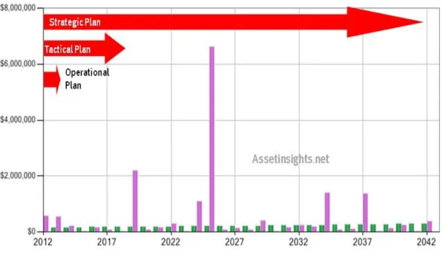
Figure 7.1 Planning Horizon ... 42
vi
LIST OF TABLES
Table 2.1 Sensitivity Analysis-Weaned Replacement Heifers Needed as a Percent of
the Number of Cows to Calve ... 10
Table 5.1 Feed Table for Conception to Weaning ... 34
Table 5.2 Feed Table for Weaning to Yearling ... 35
Table 5.3 Current and One Year Out Prices ... 36
Table 6.1 Summary for Raising Heifers with Scenario A&B ... 39
vii
ACKNOWLEDGEMENTS
I would like to thank my major professor Dr. Dustin Pendell for his continual guidance and advising throughout this entire process. I would also like to thank Deborah Kohl, Mary Emerson-Bowen, and Gloria Burgert. They have always been there cheering me on and encouraging me at every corner of the way. Each one of them has made my time in the MAB a more enjoyable one. In addition, I would like to thank my committee members Dr. Sandy Johnson and Dr. Allen Featherstone for offering their assistance and guidance as well along the way. I could not have done this without any of these
individuals.
I would like to take this time to also thank all my family and friends who have helped encourage me as I went through this journey the past two and a half years. I would especially like to thank my wife Kinsley who has supported me every step of the way and supported my decision to pursue my master’s degree. Though it was a long process and I wondered at times if this was the right decision she continued to lift and encourage me while showing me that this was meant to be. In addition, I would like to thank both my parents Richard and Sue for always believing in me and knowing that I can do anything I put my mind to. I cannot thank them enough for the continual love and support they have given over the years. Lastly, I would like to thank God for placing the desire in my heart to pursue my master’s degree and for giving me the motivation, drive, and skill set I needed to complete this task. I will be forever thankful.
1
CHAPTER I: INTRODUCTION
Sachse Family Angus is both a commercial and registered Angus cow-calf operation in Northeast Kansas and has been in operation under the Sachse family since 1935. In 2010, the Sachse Family purchased their first two purebred registered Angus heifers. Since then, the focus has shifted to expanding and developing the purebred cattle operation while maintaining their commercial herd. The end goal is to provide quality seedstock to other producers. With the addition of registered cattle, they knew they needed to focus their attention on growing their foundation Angus females. Successful selection and development of beef replacement heifers have major long term effects on stayability in any herd and can even have a positive impact on the whole herd. One issue producers have each year is finding an adequate supply of heifers that fit their herd and environment. Although there are many producers who select heifers from their own herd, often times going to a production sale, auction market, or purchasing through private treaty sales can be a good alternative for heifer selection. With today’s low livestock prices and current
agricultural economic situation, it is crucial to ensure profits are still attainable throughout the heifer selection process. Either route a rancher takes (i.e., purchasing or raising), the source of heifers needs to result in the most economical source because they can have major implications on the effective use of resources, costs, and success of remaining competitive in the cattle business.
1.1 Development Plan
According to Grussing (2016), many producers today often overlook a development plan when it comes to replacement heifers. “They just visually appraise and chose the largest heifers in the pen” says Grussing. The primary cost associated with developing
2
heifers managed under extensive conditions is purchased feed to augment diets for sufficient gains to achieve puberty before breeding (Roberts 2009). Many heifer development expenses are often overlooked. For instance, variable costs such as feeder wagon repairs, tractor, and pickup fuel are often not accounted for. With replacement heifers contributing significant costs to a ranch’s overall expenses, it is crucial to have a plan. Additionally, it is widely accepted that progressive producers who stand out among competitors are the ones who analyze and benchmark their costs year after year against industry averages. Benchmarking should be done by all ranches because it can mean the difference between net profit and net loss in any given year. As the old saying goes, “you cannot manage what you do not measure”. Therefore, producers must be flexible in terms of modifying their herd replacement strategies as needed to take advantage of changing conditions in the market and work to build a development plan that best fits their operation. 1.2 Herd Evaluation
A crucial step in developing a herd management plan is to evaluate your herd to know where you currently stand. Scott Brown of the University of Missouri says producers have to begin by evaluating their herd to determine their current herd needs. It is important to determine the genetic needs of your herd and identify what could be improved upon (Brown n.d.). Likewise, if you want to purchase heifers to add to your herd, then you have to have a firm understanding of your short- and long-term herd goals. Some producers may have high-quality carcass genetics, while others are lacking in mothering traits in their cows. Brown warns producers about having a biased opinion of their herd (Black 2016). Biased options can lead to inaccuracies in herd evaluation and possible improper
replacement selections. This can be a costly mistake because beef cow herds are very capital intensive enterprises. Whether a cattleman is purchasing his replacements or
3
developing his own group of heifers, there is an initial investment followed by a stream of future profit that will hopefully provide a return to the original investment.
1.3 U.S. Cattle Inventory
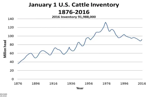
Several years ago, drought struck much of the United States causing herd liquidation. This decreased the U.S. cow herd considerably. In fact, the total U.S. cattle inventory decreased by 1.9 million head in 2011 and totaled 90.8 million head on January 1st, 2012 (CattleFax 2012). This marked the fifth consecutive year for a decline in the total cattle inventory and put the 2012 total at the smallest level since 1952. Figure 1.1 shows the dramatic decrease in cattle inventory.
Figure 1.1 U.S. Cattle Inventory 1876-2016
Source: USDA, National Agricultural Statistics Service 2016
With the drought ending and ensuing record high cattle prices, many producers have been in the process of expanding their herds again. A recent USDA report shows that
4
as of January 1st, 2017 cow numbers continue to be on the rise. The total cow numbers are the largest they have been since 2009 at 40.6 million head. As a result, the number of calving cows in 2016 was up three percent with the total number of replacement heifers increasing by one percent. Indications show that this is the largest number of replacement heifers on ranches since 1997. If weather patterns and margins hold, producers may see additional growth in 2018. In order for cow-calf producers to remain profitable, they will need to shift their focus to finding production efficiencies while controlling cow costs. 1.4 Thesis Objective
The objective of this study is to create a decision tool that will assist Sachse Family Angus in determining whether purchasing or developing their own replacement heifers is the best strategy. Specifically, this research will evaluate the cost of heifer development, ranging from conception to a yearling age of 14 months, while allowing Sachse Family Angus to apply incremental changes to their current management plan to determine if these changes are economically feasible. One change will take a look at if Sachse Family Angus develops their heifers, should they make their replacement decisions at weaning age and have development costs ranging from conception to the weaning period? Secondly, if Sachse Family Angus converts their crop ground into pasture and hay ground, does it make financial sense to develop these heifers to a yearling age of 14 months without grazing crop residue? To evaluate this objective, a partial budget is created to assist Sachse Family Angus with the impact of incremental changes have on an operation.
In addition, this study will touch on creating a Blue Ocean Strategy.Blue Ocean Strategy (BOS) is the simultaneous pursuit of differentiation and low cost to open up a new market space and create new demand (Blue Ocean Strategy 2016). This type of thinking will allow producers to stand apart from competitors while keeping cost of production low
5
allowing them to better determine if developing their own or purchasing heifers is the best option for them. A good solid development plan will help producers realize the best avenues to use their available resources. The bottom line is that because of recent low returns, it is crucial for a producer to have a solid development plan while taking into consideration alternative strategies to cut overhead costs of production. As a result, the time and effort will pay off in the long-run. In a similar way, a solid selection plan will aid the producer who plans to purchase his heifers. In turn, Sachse Family Angus will use this information to build their registered and commercial replacement heifers.
6
CHAPTER II: LITERATURE REVIEW
The depth of literature addressing the decision of buying or raising replacement heifers is vast, providing various degrees of analysis to aid a producer to make the best informed decision. Some economists would argue that no single aspect of beef production management is as complicated, or has such an economic impact as cow culling and
replacement heifer decisions (Melton, 1980). Participating in a competitive industry results in great risk that producers must accept because they are price takers in the market place. This implies that producers have little control of the price they receive for their product.
In the beef industry, females are considered both a capital and consumption good. As a result, if the price of purchasing females increases, producers may retain more heifers for their herd, thus reducing the supply of heifers into the market place. This will allow them to take advantage of the high prices they will receive in the future for selling. In the short-run, supply of heifers will be lower thus driving up the price. Producers who held onto their heifers can then capitalize on these higher prices by selling (Aadland, et al., 2001). Inversely, during periods of lower prices, the decision that often makes the most sense is to retain your own heifers. Expectations and steps need to be taken to achieve selection success.
2.1 Considerations
One goal for replacement heifers is to grow into a fertile cow that produces a calf unassisted annually for many years. Once producers have selected heifers that meet both phenotype and genotype acceptance by the producer, it is time to move them to their replacement pen or can add them to the list of potential purchases. In a study completed by Perry et al. (2009), a few rules of thumb for heifer development or selection criteria can be summarized. These include: reaching puberty by 12 to 14 months of age, conceive early
7
in the breeding season at 14 to 15 months of age, weigh approximately 65 percent of her estimated mature cow weight, rebreed in a timely manner post calving, and raise a healthy calf to weaning. All of these goals help to create a heifer that will have a long-term positive impact on the cow herd. Heifers not meeting production targets should be culled at any point in the process or scratched off of the “like to purchase list” Feuz (2002).
According to Grussing (2016), considerations should be made for future
replacement plans. Evaluating the total cost from conception to yearling age is a critical first step when taking a look at which heifers can fit the herd and can give cue’s to producers on whether or not they have the financial resources to raise or purchase. Second, budgets are essential in planning and can identify the costs per head. Producers who have a greater number of heifers to develop or buy can decrease fixed costs per head by spreading their costs over additional heifers (i.e., economies of scale). Ranchers also need to determine what resources and genetic characteristics will meet their management and production goals.
If producers have the skill, experience, and technology available, then developing heifers might be feasible. If these same producers have a disadvantage in these areas, then they should consider purchasing their replacements. Producers need to place value on time, resources, and quality into developing heifers the best way they know how; thus, ultimately improving their cowherd.
Producers who place emphasis on certain types of traits or even bloodlines may find it harder to replicate when purchasing heifers. Heifers raised on a producer’s own operation may be adapted to the management style and nutritional program that comes with being home-raised. By raising replacement heifers, a producer may be in a better
8
position to evaluate their growth, phenotype, and temperament (Gunn, 2016). Raised heifers will even be more accustomed to the management style of the producer once added to the cow herd. Producers can also cut down on potential respiratory diseases, bovine viral diarrhea, and other health issues using a closed-herd system. Often times, larger producers can raise their own heifers more economically than purchasing heifers. Producers with smaller herds may experience better margins if they purchase their replacements. Decision aides are needed to know whether, given the current market, if this is the best option or not.
Purchasing your replacements, however, may be the better option given a producers skill level and resources. If one decides to purchase, this eliminates the need for a producer to have a group of weaned calves to develop. This will in turn free up facility space, pasture, and feed that would be consumed developing these heifers. Another advantage is that producer may in fact be able to purchase heifers from those cattle breeders who specialize in developing replacement heifers for other cattlemen. These heifers will often times be sired by high accuracy calving ease bulls. These heifers are typically up to date on the correct health protocols as well as a nutrition plan.
Many ranchers often overlook heifer development in their programs. Many
producers are busy during or after weaning time with other tasks, such as crop harvest, and thus get distracted and forget that one of the most important times in the heifer’s life, between weaning and first breeding. Producers do not consider the true cost of
development. What factors or opportunity costs do these ranchers forget? Many heifer development expenses do not require producers to write a check; thus, are often
9
occur regardless of the number of heifers kept for development. The opportunity cost of buying a replacement instead of developing yourself needs to be considered as well. Additionally, the management of heifers during the development period can significantly impact her future as a cow. Research shows females who calve early in their first calving season will more than likely continue to calve early in subsequent calving seasons; thus, weaning heavier calves throughout her lifetime. In fact, Lesmeister et al. (1973) noticed the effect of relative first calving date in beef heifers on lifetime production using production records from two different herds. The study included 2,036 spring calves from 481 cows weaned in October or November of each year. Heifers calving initially in the early, first and second groups tended to calve earlier throughout the remainder of their productive lives than heifers calving initially in later groups. This study indicates the importance of managing and breeding heifers such that they will calve early in the season and then tend to maintain early calving throughout their productive lives. Such management should
contribute profit in the cow-calf operation.
2.2 Determining Number of Heifers Needed
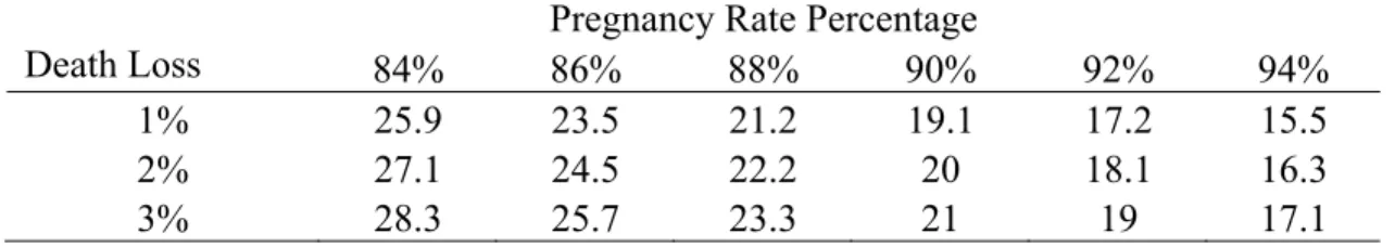
A study completed by Feuz (2002) describes how producers can determine how many heifers are needed for replacement for a herd. Fuez discusses that pregnancy rates will vary the number of heifers needed each year. Feuz further suggests replacement rates of 15 to 25 percent are very common for most producers, but can range from 10 to 30 percent. Table 2.1 features a sensitivity analysis of the number of heifers needed for
replacement varying by death loss and pregnancy rate; however, culling decisions were not factored into the table. Using table 2.1, if a producer has 100 cows, an 84% pregnancy rate,
10
and a 3% death loss, the rancher would need 29 heifers for replacement. If death loss can be minimized and pregnancy rate can be improved, then fewer heifers are needed.
Table 2.1 Sensitivity Analysis-Weaned Replacement Heifers Needed as a Percent of the Number of Cows to Calve
Death Loss
Pregnancy Rate Percentage
84% 86% 88% 90% 92% 94%
1% 25.9 23.5 21.2 19.1 17.2 15.5
2% 27.1 24.5 22.2 20 18.1 16.3
3% 28.3 25.7 23.3 21 19 17.1
Source: Feuz (2002) 2.3 Blue Ocean Strategy
Once a producer determines the number of replacement heifers needed in their herd, it is time to think about the kind of market that those heifers are in. If these heifers are being sold, effective marketing that maximizes their value potential is key. If heifers are purchased at an auction market, via private treaty or through a production sale, the price paid for these heifers will be different at each respective market. In fact, producers should consider using strategies that are present in Blue Ocean Strategy (BOS) to better
understand the type of market these heifers are in. According to research by Krishnan (2016), BOS generally refers to the creation by a business of a new, uncontested market space that creates new value while decreasing costs. In order to find this uncontested market place, Mauborgne and Kim (2016) argue that businesses should give consideration to the “Four Actions Framework”. According to Mauborgne and Kim (2016) the four actions framework is used to reconstruct buyer value elements in crafting a new value curve or strategic profile. At the heart of BOS, it focuses on those who pursue product differentiation and who are low cost producers. Four questions arise: 1) What factors should be raised well above the industry standard?; 2) Which factors that the industry has
11
long competed on should be eliminated?; 3) Which factors should be reduced well below the industry’s standard?; and 4) Which factors should be created that the industry has never offered? Value innovation is the successful recombination of resources to reduce supplier cost and/or increase value in use, and can be a game changer for any ranch if implemented properly no matter if the producer is developing his own heifers or purchasing. Producers who constantly think outside the box will set themselves up to explore and attain market boundaries that others can only imagine through the use of technology. Thirdly, if producers use BOS in their heifer development plan, they will be maximizing their opportunity while minimizing surprises and risks.
2.4 Strategy Canvas
Building a quality cow herd requires significant investments of time, money, and dedication. The strategy canvas, an all-important analytical tool that is an integral part of BOS, can transform hopes about the market place into objectives leading to discovery. The strategy canvas is a central diagnostic tool and an action framework developed by
Mauborgne and Kim (2016) for building a compelling BOS. Research from other industries may also apply to helping ranchers build a quality cow herd.
In a study conducted by Khalifa (2009), a strategy canvas was designed for a business school based on students’ perceptions of the importance of critical value dimensions of its undergraduate offerings and its performance of each. A survey was conducted and used to measure students’ perceptions. The findings show the strengths and weaknesses of the school’s current strategy profile. These findings suggest how to best use available resources to improve performance and trigger value innovation. It shows how the
12
strategy profiles of competitors compare and where to look for further information. This in turn helps to create new strategic insights.
These are just some of the things a producer needs to consider when creating a replacement heifer development plan or implementing when selecting heifers. Having a heifer development plan and selection criteria can help producers determine the best use of their resources. This is especially true when there are expectations of lower profit margins as a result of depressed market prices. Ultimately, a successful heifer development program and selection criteria for buying can result in a profitable cowherd that will be around long into the future.
2.5 Replacement Heifer Strategies
A research study conducted by Freetley et al. (2001) determined primiparous heifer performance that affected pregnancy percentages following three different heifer
development strategies that were the result of timed nutrient limitation. Two hundred eighty-two spring-born U.S. Meat Animal Research Center heifers were weaned around 203 and 205 days of age. Treatments consisted of different quantities of the same diet being offered for a 205-day period. Heifers received 263 kilocalories (kcal) (HIGH), 238 kcal (MEDIUM) or 157 kcal (LOW-HIGH) of metabilizable energy (ME) per unit of metabolic body weight (BWkg)0.75 daily for the first 83 days. Heifers in the low-high treatment were offered 277 kcal ME/(BWkg)0.75 daily for the remainder of the 205-day period whereas the high and medium groups remained at a constant level of energy. After the 205 day feeding period, heifers were taken out of the drylot and placed in breeding pastures.
They found that the percentage of heifers that calved expressed as a fraction of the cows exposed did not differ among treatments (89.7%; P = 0.83). The age of heifer at parturition (P = 0.74) and the time from first bull exposure to calving (P = 0.38) did not
13
differ among treatments. Calf survival was lower in the low-high treatment than the medium, but similar to those on the high treatment. These findings suggest that as long as heifers are growing and meet a minimal breeding weight before mating, patterns of growth may be altered in the post-weaning period without a decrease in the ability of the heifer to conceive or a decrease in calf growth potential. These alterations in post-weaning gain through monitoring the amount of feed offered can be used to optimize feed resources.
In a study conducted by Marsh, Jones, and Terry (1999), a partial budget was used to compare alternative strategies to raising replacement heifers. A heifer production calendar was presented which outlined costs over a period of time. The study concluded from the partial budget that those who raise heifers can incur significant opporuntity costs. It is emphasized that varying alternative strategies, such as selling heifer calves at weaning and purchasing heifers, may offer lower cost alternatives. Finally, those producers with a comparative advantage, for example better genetics and facilities, are likely to find raising heifers an optiomal strategy.
In conclusion, maintaining a high quality beef cow herd means selecting and developing quality replacement heifers to retain in the herd each year. When managing home raised heifers or purchased heifers, maintaining costs and keeping them in check is crucial because they represent a large up-front investment. The bottom line of this research is to give producers a decision tool that can be used to analyze their current resources and help them analyze if purchasing their heifers or developing their own makes the most financial sense.
14
CHAPTER III: THEORY
Drought conditions in 2012 shrunk the national cow herd to record low numbers resulting in record high beef cattle prices. With record high prices and increasing profits the past couple of years, cattlemen have been investing in expensive replacements females, via raising or purchasing, without consideration of the long-term negative impacts this could have on an operation. Since then, prices have come back down to a more stabilized level. As margins are smaller today when compared to a couple of years ago, this study will focus on the costs associated with replacement heifers (Pendell and Herbel, 2016). ‘What are heifer’s worth?’ is a fundamental question that is often times determined by the markets. Because this question is difficult to answer and out of the producer’s control, this study will discuss different scenarios spurring thought to help the producer make the best informed decisions for their long term herd goals.
3.1 Perceived vs. Actual Value
Is the perceived value of an animal the same thing as what it is really worth? More often than not, the answer is no. Often times, the value of raised replacement heifers and what price someone will buy or sell quality replacement heifers may not be the same dollar value (Lemenager and Lake, 2015). It is wise to not over-value heifers or place a higher value on them than they actually are worth. If selling heifers, some
producers may have a high actual value on their heifers while other producers view those heifers with a low perception value. This reasoning can be helpful to producers wanting to determine actual and perceived costs associated with buying replacements from other ranches. The same holds true for ranchers developing their own heifers and over valuing them and their genetic merit. Furthermore, what actual input costs and output prices are going to be in the future is really what needs to garner focus. Annual costs associated
15
with replacements heifers will always vary from operation to operation and from year to year, and include both fixed and variable expenses.
3.2 Calculating Costs
Determining costs involved in the whole heifer development period, conception through point of sale, needs to include opportunity costs and not just cash costs. There are six steps in calculating the cost of developing home-raised heifers (Hughes 2005). First, a producer will need to place a market value on their own raised heifers. For those producers who retain ownership of their calves through backgrounding can extend costs to yearling age. The market value will essentially be the weight of the animal, at weaning or yearling age, multiplied by the market price. Second, during the time period of weaning to breeding, a producer will want to calculate his wintering cost, late spring grazing costs, and cost of gain over that time period. There are two common ways a producer can winter heifers: feed them grain, hay, high roughage diet in a drylot setting, or on dormant range with stockpiled forage and supplement.
In a study completed by Perry et al. (2009), they suggest a continuous supply of correctly developed heifers is crucial to the success of any cattle operation. Following breeding, the way in which heifers are managed can have big implications on the reproductive performance and lifetime productivity of replacements heifers. Perry et al. (2009) found that heifers developed in a feedlot from weaning to breeding experienced lower average daily gains in the subsequent summer compared to forage grown heifers. In their study, they concluded there is decreased pregnancy success in feedlot developed heifers moved to grass immediately following insemination. Producers should make careful considerations and realize there are implications on pregnancy success if diet changes occur immediately after breeding.
16
Next, the producer needs to record expenses during the time period of breeding to pregnancy checking. Things such as pasture rent, mineral and breeding costs are included here. This step would be important if developing bred replacement heifers. The focus of this study, however, is on developing heifers to yearling age right before breeding season starts. Fourth, all the expenses associated with raising replacement heifers are summed. Fifth, a producer will need to adjust for heifer pregnancy rate. To do this total expenses, including opportunity costs, are divided by the achieved conception rate. Lastly, a producer needs to adjust for open cull heifer credits. However, steps five and six do not apply to this research. Due to lack of pasture availability, Sachse Family Angus only records expenses from conception through open yearling age around 14 months because that is when the decision is made whether to purchase or keep the heifers in the herd. At this point, the decision makers cull the heifers they do not plan to keep on their operation.
3.3 Enterprise and Partial Budgeting
Bradford and Debertin (1985) describe enterprise budgeting as a simple technique that can be easily applied to any operation. Enterprise budgeting is the systematic
determination and listing of expected outputs, revenues, and costs due to the production processes required to produce one unit of an enterprise for a specified time period. Enterprise budgets are based on production theory, specifically marginal analysis and capital theory (Bradford and Debertin, 1985). Unfortunately, these budgets may be complex and foreign to the average cattleman who makes a budget.
Bradford and Debertin (1985) discuss six sets of issues and questions producers need to be aware of. First, the term enterprise budget should be well defined and differs from other types of budgets (e.g., cash flow, partial, and whole farm). Secondly, how does one account for different ranch sizes when budgeting for a single ranch enterprise? Thirdly,
17
what output level, or number of heifers produced, is appropriate for a basic budget? In addition, is the current output level optimal? Fourth, is enterprise budgeting considered a planning tool or a historical accounting exercise? Fifth, should the budgeted values be real or nominal? Nominal values are often times an approximation and real or actual values are calculated and exact. Careful considerations should be made because inflation projections could be the main reason for building the budget. In neoclassical production theory, it is assumed the producer makes choices with respect to the combination of productive factors and products.
According to Mitchell (2017), partial budgets can be an important part of enterprise budgeting. In essence, partial budgets take an enterprise budget one step further. Enterprise budgets are important to estimate profitability on a ranch while documenting management practices and the resources that are used in the production of heifers, partial budgets can aid a producer who is interested in taking a look at making a change to his management
practices. Partial budgets include an analysis of net returns from small changes or refinement to a ranch. It focuses on components that change while building upon an enterprise budget. In essence, it fine tunes current operations while holding all else constant. The benefit of partial budgeting is that it takes a look at what will be the new or added revenue if a change is implemented on the ranch. Additionally, a partial budget also looks at and what costs will be reduced or eliminated if taken place (Figure 3.1). What will be the new or added costs and what revenues will be reduced if a change takes place are also things to consider. The results will demonstrate to a ranch manager the net benefit of the change.
18 Figure 3.1 Partial Budget: Defining the Change
Benefits Costs
Additional Revenues
What will be the new or added revenues?
Additional Costs
What will be the new or added costs?
Costs Reduced
What costs will be reduced or eliminated?
Revenues Reduced
What revenues will be reduced or lost?
Total Benefits Total Costs
Net Benefit
Using a marginal framework will allow the decision maker to optimize inputs and outputs. Enterprise budgeting can result in an approximate solution to marginal analysis if an array of budgets can be made with the proper amounts of inputs and outputs. Marginal analysis can be described as taking a look at both the benefits and costs of different alternatives and the incremental changes on total revenue and total costs caused by small input and output changes. Because these incremental effects can lead to change, it is imperative a budget should be constructed for different ranch sizes with each ranch as a series of budgets that would cover all possible ranges of inputs or output levels. Using marginal analysis, a producer can solve for an optimal production level.
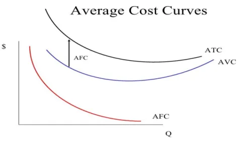
A producer can add a hypothetical unit cost and revenue curve for buying or raising heifers. This graph would consist of average variable costs (AVC), average fixed cost (AFC), and average total costs (ATC). The AVC curve represents a set of variable inputs that are assumed to be combined to produce a replacement heifer. The AFC curve
19
represents a selected size of a ranch. ATC then represents the combination of both AFC and AVC (Figure 3.2).
Figure 3.2 Average Cost Curves
When creating a cost and return per animal unit budget, it is important to list variable costs first in order to show a one year planning horizon and the fact that the producer has dedicated certain resources to the production of a replacement heifer. Often times, a producer will need to make a quick decision and use the information from a single budget to make a decision. For example, if the planning horizon is shortened because of losses to some replacement heifers unexpectedly, the rancher will need to make a quick decision to replace them. They will then only focus on variable costs such as buying heifers. However, problems can arise from labeling costs as only variable and fixed. The costs of inputs that provide services for more than one production year can alternatively be labeled as long-run costs. The costs of inputs which will provide services for only the current year are designated as short-run costs.
Two issues arise when thinking about time value of money and inflation. The first issue is whether to use nominal or real dollar units. Secondly, what procedure should
20
producers use to account for the replacement of durable inputs? Enterprise budgets can either be designed to capture a single selected year or a typical year. Input price inflation is usually not uniform among inputs over time. Because inflation is difficult to predict and this study does not take a look at budgets over several years, it makes sense to prepare a budget using nominal values. Additionally, nominal prices, also called current dollar prices, are more accurate depiction of a price at the time a product is made or sold.
Decision makers must be aware that enterprise costs and returns can widely vary across location and years. Changes occur because of technology, weather, and a producer’s managerial skills. Because of this, an enterprise budget is more or less a cost and return tool and the unit curves on the graph will shift upward or downward depending on market conditions and production level. For example, if technology improvements such as new genomic DNA testing are made available allowing producers to more easily select and develop heifers, then production theory tells producers that the cost curves will shift downward. The reduction in costs will lead to an increase in the supply at each price level, causing the product price and marginal revenue curve to shift downward. In addition, there remains a problem of continuing to update cost relations of enterprise budgets.
21
CHAPTER IV: METHODS
It is important to lay the ground work before we discuss the methods used to solve the question at hand: should a producer develop their own heifers or purchase
replacements? It is crucial to discuss the fact that low cost producers are not necessarily the high profit producers, but rather these producers are able to maintain profit margins.
Pendell and Herbel (2016) divided cow-calf net returns for the 2011 to 2015 period into high-profitable (HP), medium-profitable (MP), and low profitable (LP) operations based on annual net returns over costs. This analysis showed that HP operations had a $307 per cow advantage over LP and $146 per cow advantage over MP. Additionally, combining gross income and cost advantage, HP producers had $398.49 advantage over LP operations and $187.48 advantage of MP operations. HPs had larger cow herds, sold heavier calves, and were more efficient with labor than their LP counterparts. In addition, HP producers, on average, had a cost advantage in all categories.
According to Laudert (2012), higher total cow costs equates to lower profits with the primary driver being feed costs, which were by far the greatest difference between high and low profit producers. In fact, feed costs were about half of all total costs. It goes without saying that if a producer can control feed cost they can become a more profitable producer. The producer’s management of non-feed costs is also important. Interest and labor rank high as well between these two types of producers. Machinery costs typically represent a strong positive correlation meaning if a rancher can keep these costs lower then they will be more profitable in the long run. Lastly, and certainly not least, are a producer’s herd size and whether or not a producer specializes in livestock or is more diversified and has a farming side of the operation as well. One can reason that a larger herd can spread
22
fixed costs over more animals reducing costs per head. In addition, producers focusing solely on livestock rather than diversified operations tend to be more profitable too (Kime and Hyde, 2017). In conclusion, cost of production is a critical component in determining if someone is a high or low profitable operation. It should be noted that benchmarking against other producers is a good practice to gauge where a ranch has been, where it is going, and where it is headed.
In addition to using the Cow Herd Appraisal Performance Software (CHAPS), producers can use Porter’s Generic Competitive Strategies (Porter, 1985; Figure 4.1) to benchmark their costs against others in the same industry is to use. In this strategy, there are two types of advantages a firm can possess: low cost and differentiation. Producers can utilize these with three additional strategies to help them out perform the competition. These three additional strategies include cost leadership, differentiation, and focus. The focus category can have either a cost focus or differentiation focus.
23 Figure 4.1 Cost Differentiation
Source: Porter’s Generic Strategies
Cost leadership is when an operation sets out to become the lowest cost producer within the industry. Some of these producers can capture this because of economies of scale or have special access to new technology or other resources. In differentiation, producers seek to be unique in the industry with products that are highly sought after by customers. It holds up industry important products, in this instance heifers, and positions them to market to customers who are willing to pay for this differentiated product. Focus describes producers who solely tailor their product (i.e., replacement heifers) to a group of producers. Focus is further divided into cost focus and differentiation focus. In cost focus, producers strive to capture a cost advantage within their targeted group. In differentiation focus, producers seek to differentiate within its targeted group. These targeted groups
24
capitalize on buyers with unusual needs that are sometimes superior or else the production can differ greatly compared to others in the industry.
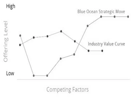
Another tool for benchmarking is the strategy canvas. It graphically captures the current strategic landscape and the future prospects for a ranch (Figure 4.2).
Figure 4.2 Blue Ocean Strategy Canvas
Source: Mauborgne and Kim (2016)
This strategy canvas can serve two purposes for producers. The first, according to Mauborgne and Kim (2016), is to capture the performance for the individuals in the industry. As a result, producers can see the factors at play within the industry as well as where the competition is investing. The second purpose is to allow producers the ability to reorganize their focus so they can best compete within the industry. The vertical axis shows the offering level income that buyers receive across the different heifer development types.
25
As stated, the horizontal axis represents factors that an industry competes on and invests in. The value curve is a graphic depiction of a ranch’s relative performance across its
industry’s factors of competition.
With the ground work laid out, this study will now discuss the decision aid tool. This decision aid tool was created to assist Sachse Family Angus in making the decision between purchasing replacements or raising their own heifers. This tool is on a per-head basis over the period of time from conception to a heifer’s yearling age. This tool is made in such a way though that the producer can change the time period that correlates to their operation. In addition, a producer can analyze what different time periods look like in relation to their operation. This tool helps producers who typically have the resources, ability, and know how to raise their own heifers, but are looking to purchase their replacements if it is cheaper than raising their own. Secondly, this tool will help those producers who usually go and buy their replacements, but might consider raising their own. 4.1 The Decision Tool
To make the decision tool functional, the producer must know their resource base and be able to budget. More specifically, this tool is a partial budget with components of an enterprise budget that helps ranchers evaluate the financial effect of incremental changes in their operations. This tool is valuable for analyzing proposed adjustments within an
operation. It is important to remember that this tool can provide a glimpse into different scenarios that can determine whether it is best to purchase or raise replacement heifers. This spreadsheet is split into two categories: positive impacts and negative impacts. Positive impacts include added returns and reduced costs while the negative impacts include added costs and reduced returns. If returns exceed costs, then the analysis will increase net returns and be a beneficial activity for the producer. Inversely, if costs surpass
26
returns, then the analysis will decrease net returns and will not be an activity a producer will want to pursue. Certain returns and costs are not known to the producer in future time periods such as sale price of a heifer calf and costs of a purchased heifer. Cow-calf
producers wanting to make business decisions will most likely base the analysis on the most likely assumptions during the future heifer development period.
This decision tool analyzes several factors that are of critical importance. A producer using the tool will want to make sure they do not forget to include items such as depreciation, taxes, insurance, and interest costs. Though the spreadsheet will work for anyone, ranchers will want to focus on being a low cost producer to try and maximize their profits. It should also be noted that the values in the spreadsheet will look differently for each producer because income and costs are not the same for two producers. While producers cannot control volatile market prices, they can, however, have more control of their input costs.
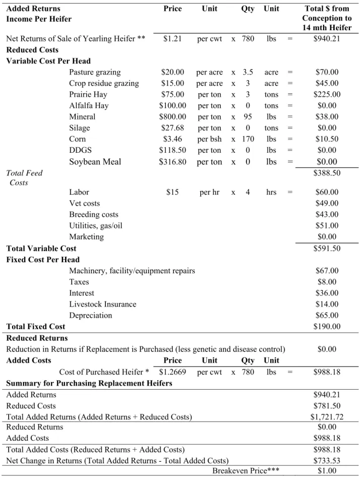
To begin, a producer will need to develop an alternative marketing strategy to what they are already doing. For instance, if heifers are sold at yearling age, the producer can analyze what selling heifers at weaning age looks like. Sachse Family Angus would like to analyze what buying replacements looks like when they have historically raised their own (Figure 4.3). The producer will first see the positive impacts category or the added returns and reduced costs. A producer will begin by incorporating their expected returns from the sale of heifers into the budget. The returns include the net returns from the sale of a weaned heifer calf. To properly calculate the price of the sale of a heifer, the producer will multiply the weight of the animal by the expected market price at the time of sale. For this thesis, $120.54 per hundred pounds (cwt) was obtained from Beef Basis.com. Farmers and
27
Ranchers Livestock Auction Market was the location used as it is the closest auction market in proximity to Sachse Family Angus. March 15th, 2017 was the date used on the contract because mid-March is often times when Sachse Family Angus determines whether to keep their replacements or to buy. The spreadsheet uses 780 pounds for the heifer
because this is the target weight for Sachse Family Angus heifers at breeding time. The next section is the reduced costs. Variable costs include both feed and other costs. Feed costs include: winter feed costs, crop residue grazing, prairie and alfalfa hay, salt and mineral, silage, corn, DDG’s, and soybean meal. Other variable costs include labor, vet costs, breeding costs, marketing, utilities, gas and oil. Fixed costs include items such as: machinery repairs, taxes, interest, livestock insurance and depreciation. The reduced costs total $781.50 (i.e., variable and fixed costs are $591.50 and $190, respectively). Summing the added revenue and reduced costs from buying replacement heifers instead of
developing generates $1,721.71.
The producer can now calculate the negative impacts of buying versus raising replacement heifers. Within this section, the impact includes reduced returns and added costs. The reduced returns are the reduction in returns if a replacement heifer is purchased. In this scenario, the reduced returns are zero if the replacement heifer quality is lower than what could have been kept from within the producers herd. The increased costs are the purchase of a replacement heifer. It is assumed the cost of the replacement heifer is the cash market price of a similar weight steer and multiplied by the weight of 780 pounds. There have been several instances where open replacement quality heifers have been marketed for the same price as same weight steers (Griffith, 2015). In this scenario, the cash steer price is $126.69 per cwt resulting in a heifer purchase price of $988.18. This
28
cash price was achieved by using a March 15th, 2017 contract date from Beef Basis.com using 780 pounds. The sum of added costs of $781.50 and reduced returns of $940.21 result in the negative impacts associated with buying versus raising heifers.
The final step to evaluate the potential change in the production practice (i.e., purchasing vs. raising) is to subtract total added costs from total added returns. The end result is a net change in returns. If the number is positive, the partial budget suggests it makes sense to purchase while a negative value indicates a producer is better off raising heifers. Finally, to calculate a breakeven out price, the producer will add the total fixed costs to total variable costs and divide by quantity or production unit. This would give the producer a price in cwt.
29
Figure 4.3 Partial Budget-Purchasing Replacement Heifer
Added Returns Price Unit Qty Unit Total $ from
Conception to 14 mth Heifer Income Per Heifer
Net Returns of Sale of Yearling Heifer ** $1.21 per cwt x 780 lbs = $940.21
Reduced Costs
Variable Cost Per Head
Pasture grazing $20.00 per acre x 3.5 acre = $70.00
Crop residue grazing $15.00 per acre x 3 acre = $45.00
Prairie Hay $75.00 per ton x 3 tons = $225.00
Alfalfa Hay $100.00 per ton x 0 tons = $0.00
Mineral $800.00 per ton x 95 lbs = $38.00
Silage $27.68 per ton x 0 tons = $0.00
Corn $3.46 per bsh x 170 lbs = $10.50
DDGS $118.50 per ton x 0 lbs = $0.00
Soybean Meal $316.80 per ton x 0 lbs = $0.00
Total Feed Costs $388.50 Labor $15 per hr x 4 hrs = $60.00 Vet costs $49.00 Breeding costs $43.00 Utilities, gas/oil $51.00 Marketing $0.00
Total Variable Cost $591.50
Fixed Cost Per Head
Machinery, facility/equipment repairs $67.00
Taxes $8.00
Interest $36.00
Livestock Insurance $14.00
Depreciation $65.00
Total Fixed Cost $190.00
Reduced Returns
Reduction in Returns if Replacement is Purchased (less genetic and disease control) $0.00
Added Costs Price Unit Qty Unit
Cost of Purchased Heifer * $1.2669 per cwt x 780 lbs = $988.18
Summary for Purchasing Replacement Heifers
Added Returns $940.21
Reduced Costs $781.50
Total Added Returns (Added Returns + Reduced Costs) $1,721.72
Reduced Returns $0.00
Added Costs $988.18
Total Added Costs (Reduced Returns + Added Costs) $988.18
Net Change in Returns (Total Added Returns - Total Added Costs) $733.53
30
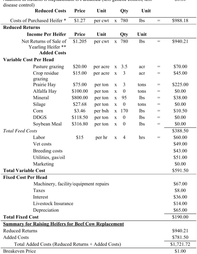
The next step is to evaluate, developing heifers when a producer has historically purchased replacements (Figure 4.4). A producer will start out by looking at added returns with the addition in returns if replacements are purchased. Next, a producer will look at the reduced costs in relation to the purchase of a replacement heifer. The steer price of $126.69 per cwt was obtained using a contract date of March 15th, 2017. Then, $126.69 is
multiplied by 780 pounds to arrive at a total revenue of $988.18. The next step is to evaluate the reduced returns. To calculate the sale of a producer’s heifer, we assume the heifer is sold in March at a price of $120.54 per cwt and multiplied by the sale weight of 780 pounds. The result is a reduced return of $940.21 per head. Evaluating added costs are the next step with variable and fixed costs being $591.50 and $190 per head, respectively.
31
Figure 4.4 Partial Budget-Developing Replacement Heifers
Added Returns Total $ from Conception to
14 month old Heifer Addition in Returns if Replacement is Purcahsed (less genetic control, less
disease control)
$0.00 Reduced Costs Price Unit Qty Unit
Costs of Purchased Heifer * $1.27 per cwt x 780 lbs = $988.18
Reduced Returns
Income Per Heifer Price Unit Qty Unit Net Returns of Sale of
Yearling Heifer **
$1.205 per cwt x 780 lbs = $940.21
Added Costs Variable Cost Per Head
Pasture grazing $20.00 per acre x 3.5 acr = $70.00
Crop residue grazing
$15.00 per acre x 3 acr = $45.00
Prairie Hay $75.00 per ton x 3 tons = $225.00
Alfalfa Hay $100.00 per ton x 0 tons = $0.00
Mineral $800.00 per ton x 95 lbs = $38.00
Silage $27.68 per ton x 0 tons = $0.00
Corn $3.46 per bsh x 170 lbs = $10.50
DDGS $118.50 per ton x 0 lbs = $0.00
Soybean Meal $316.80 per ton x 0 lbs = $0.00
Total Feed Costs $388.50
Labor $15 per hr x 4 hrs = $60.00
Vet costs $49.00
Breeding costs $43.00
Utilities, gas/oil $51.00
Marketing $0.00
Total Variable Cost $591.50
Fixed Cost Per Head
Machinery, facility/equipment repairs $67.00
Taxes $8.00
Interest $36.00
Livestock Insurance $14.00
Depreciation $65.00
Total Fixed Cost $190.00
Summary for Raising Heifers for Beef Cow Replacement
Reduced Returns $940.21
Added Costs $781.50
Total Added Costs (Reduced Returns + Added Costs) $1,721.72
32 4.2 Different Scenario’s
Partial budgets allow producers to investigate different scenarios. The time period of Scenario A, conception to yearling age, is what Sachse Family Angus utilizes in their budgets each year and this management philosophy works for them. However, this scenario may not work for ranchers in other areas of the country, state, or even region. For example, a common practice is to sell cattle after weaning. Scenario B will analyze raising a heifer from conception through a 30-day weaning period and then selling the heifer. More
specifically, the cow will be bred in April 2016, calve in January 2017, and wean her calf in October 2017. The calf will go through a short 30-day weaning period and then sold in November of 2017. Scenario C will look at the same situation as Scenario A, but this producer will not be utilizing corn stalks. As a means for expansion of their cow herd, Sachse Family Angus has considered converting their crop acreage into pasture and hay acreage. As such they would not have crop residue grazing available. This evaluation would help determine if such a change should be pursued. Costs will still range from conception to 14 months of age on the heifers.
In summary, all cattle are worth the current market price and anything above or below this price is considered perceived value. Conservative input and output price
projections need to be considered in replacement heifer budgets. This spreadsheet does not incorporate risk, but this is an important factor to consider in addition to this tool. Whether a rancher purchases their heifers or develops them depends on that ranchers risk tolerance level. This tool helps producers budget and set goals. The proper selection of heifers is an important decision and should not be taken lightly. In fact, it can affect the direction and future of the cow herd. This spreadsheet is not a one size fits all tool, but rather helps each producer individually and these decisions should be made independent of other cattle
33
operations. This tool is also not to be used as the sole avenue for selection, but should rather supplement how the producer is already making decisions. Because the future of the herd depends on successful decisions, the producer would be advised to consult an industry professional such as their veterinarian, a nutritionist, or county extension agent in addition to using this decision aid.
34
CHAPTER V: DATA
The objective of this thesis is to determine if a producer should buy replacement heifers or develop from within their herd. To evaluate this objective, a partial budget was created to assist ranchers with the impact of incremental changes on an operation. To assess feasibility, cost data was obtained and placed in the decision aid tool to subtract both fixed and variable expenses from the income to calculate net profit per heifer.
Data used in this thesis was collected from Sachse Family Angus budgets, Kansas State University’s Ag-Manager.info, and BeefBasis.com. Table 5.1 reports the estimated feed amounts for Sachse Family Angus for the period of conception to weaning. In this scenario, these amounts are what the cow is eating from the time of conception in April 2016 until the calf is weaned in October of 2017.
Table 5.1 Feed Table for Conception to Weaning
Type Quantity Unit
Pasture 3.5 total acres per year
Crop Residue Grazing 2 total acres per year Prairie/Brome Hay 2.25 total tons per year
Alfalfa hay 0 total tons per year
Silage 0 total tons per year
Corn 50 total pounds per year
Soybean Meal 0 total pounds per year
DDGS 0 total pounds per year
Protein Supplement 50 total pounds per year
Salt/Mineral 65 total pounds per year
Source: Kansas State University AgManager.info and Sachse Family Angus
Table 5.2 reports feed amounts associated with the calf at weaning time in October, through a 60-day weaning period and then grazing crop residue until 14 months of age in March of 2018.
35 Table 5.2 Feed Table for Weaning to Yearling
Type Quantity Unit Days Total Unit
Pasture 0 total acres per year x 0 0 acres
Crop Residue Grazing 1 total acres per year 90 1 acres
Prairie/Brome Hay 10 pounds per day x 150 0.75 tons
Alfalfa hay 0 pounds per day x 150 0 tons
Silage 0 pounds per day x 60 0 tons
Corn 2 pounds per day x 60 120 pounds
Soybean Meal 0 pounds per day x 60 0 pounds
DDGS 0 pounds per day x 60 0 pounds
Protein Supplement 0 pounds per day x 60 0 pounds
Salt/Mineral 0.2 pounds per day x 150 30 pounds
Source: Kansas State University AgManager.info and Sachse Family Angus
At this time, the decision is made whether to sell the heifer and buy replacements or keep her as a replacement in the herd. In both tables, pasture grazing, crop residue grazing, brome hay, corn, protein supplement, salt, and mineral were all estimated from any given year at Sachse Family Angus. These tables are not a one size fits all and will differ from year to year and operation to operation. Next, a prices tab was created (Figure 5.3).
36 Table 5.3 Current and One Year Out Prices
Source: Kansas State University AgManager.info, Master Price list, and BeefBasis.com The obtained feed price information was from the Kansas State University’s
AgManager.info master price list that was updated March 1st, 2017. A current price column as well as a one year out projection was included so producers can make more informed decisions and even plan ahead to get a projection of what the future may hold. The March steer and heifer cash price for the current year as well as a one year out projection are included to calculate the estimated price if a producer purchases their replacements and what the estimated price of selling may be. The steer and heifer prices were obtained from BeefBasis.com. The scenario of a 780 pound medium to large frame yearling heifer sold at the Farmers and Ranchers Livestock Commission in Salina, Kansas on March 15th, 2017 was used to find the March heifer cash price. An estimated mature cow size for Sachse Family Angus is 1,200 pounds and knowing that producers may elect for their breeding age heifers to be 65 percent of their mature cow size, 780 pounds in this scenario was achieved.
Current Prices One Year Out Prices
(as of March 1st, 2017) (as of March 1st, 2017)
Corn ($/bu) * $3.46 $3.80
Soybean Meal ($/ton) * $316.80 $319.10
DDGS ($/ton) * $118.50 $130.08
Pasture Rental ($/acre) * $20.00 $20.40
Silage ($/ton) * $27.68 $30.38
Prairie Hay ($/ton) * $75.00 $71.35
Alfalfa Hay ($/ton) * $100.00 $109.77
Crop Residue Grazing ($/acre) * $15.00 $15.30
Beef Cow Mineral ($/ton) * $800.00 $816.00
Other Beef Mineral ($/ton) * $550.00 $561.00
(as of March 15th, 2017) (as of March 15th, 2017)
March Heifer Calf Price ($/cwt) ** $120.54 $111.69
March Steer Calf Price ($/cwt) *** $126.69 $117.84
(as of March 22nd, 2017)
November Heifer Calf Price ($/cwt)**** $127.29
37
In this scenario, a producer will see a futures price and a basis on Beefbasis.com. To arrive at the desired cash price, the basis of this heifer was subtracted from the futures price. This results in a cash price of $120.54 per cwt. For a producer to find the one year out March heifer cash price they will run the scenario again only this time changing the contract date from March 15th, 2017 to March 15th, 2018 on BeefBasis.com. This gives them a cash price of $111.69 per cwt. To estimate at a March cash steer price, a producer will incorporate the same information using a 780 pound medium to large frame yearling steer sold at the Farmers and Ranchers Livestock Commission in Salina, Kansas on March 15th, 2017. The result is a cash price of $126.69 per cwt. Following a similar procedure the March 15th, 2018 steer cash price is $117.84 per cwt. Finally, the November 2017 heifer and steer cash prices can be found in a similar method, except the weight will change to 550 pounds. The estimated cash November heifer and steer prices were $127.29 per cwt and $137.19 per cwt, respectively.
38
CHAPTER VI: RESULTS
Partial budgeting gives producers the opportunity to analyze different scenarios. This allows the producer to gauge if there are other production practices that make financial sense. Scenario B examines the feasibility if the producer sells their calves after a defined weaning period and does not background the calves to a heavier weight. In this situation, the producer breeds their cows in April 2016, calves in January 2017, and weans in October 2017 for 30 days at which time he sells or decides to keep as replacements. Specifically, the producer will calculate his added returns or additions in returns if the heifer is purchased. Next, the producer will figure their reduced costs or the costs of a purchased heifer if the producer has historically developed their own. In this scenario, the cost of the heifer will be the same as it was in Scenario A because they will still purchase their heifers from the same reputable breeder during the same time of the year. In this case, the cost of the heifer is still $988.18 per head. Next, the producer will factor in his reduced returns or the sale of his heifer. This time they will multiple the weight of the heifer, 550 pounds, by the November 2017 expected cash heifer price of $127.29 per cwt. This will result in a $700.09 income per heifer.
Table 6.1 summarizes raising heifers for scenario A and scenario B. Reduced returns are $940.21 for scenario A, where producer sell their heifers around yearling age; and $700.10 for scenario B, where producers sell their heifers at weaning age. These amounts show what the producer could have achieved had they sold their heifers at the various times of the year. Scenario A has a higher revenue because producers would be selling at yearling age in March vs. weaning age during the fall so heifers would be larger. Because of the historical cattle cycle, prices are often higher in March vs. fall because there
39
are fewer heifers going to market. Added costs for scenario A are $781.50 and $573 in scenario B. In scenario A, producers are keeping their heifers longer so will have more expenses.
Table 6.1 Summary for Raising Heifers with Scenario A&B
Scenario A Scenario B
Total $ from Conception to 14 month old Heifer
Total $ from Conception through Weaning Summary for Raising Heifers for Beef Cow Replacement
Reduced Returns $940.21 $700.10
Added Costs $781.50 $573.00
Total Added Costs (Reduced Returns + Added Costs) $1,721.72 $1,273.10
Breakeven Price $1.00 $0.73
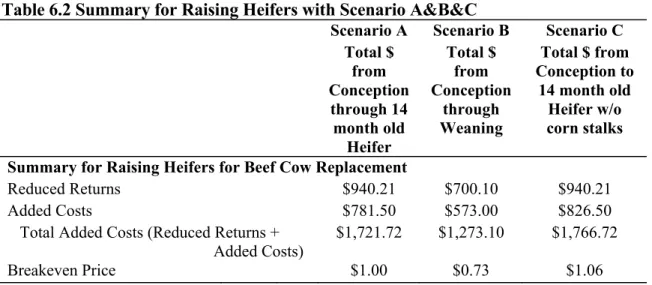
Scenario C represents producers who sell their heifers at 14 months old in March, but backgrounds those heifers not on corn stalks, but develops them with more hay. Holding all else constant, the only thing that changes in this scenario with that of scenario A is that the producer will not have any crop residue grazing expenses and will be feeding additional hay. Table 6.2 summarizes raising heifers for Scenario A, B, and C.
Table 6.2 Summary for Raising Heifers with Scenario A&B&C
Scenario A Scenario B Scenario C Total $ from Conception through 14 month old Heifer Total $ from Conception through Weaning Total $ from Conception to 14 month old Heifer w/o corn stalks Summary for Raising Heifers for Beef Cow Replacement
Reduced Returns $940.21 $700.10 $940.21
Added Costs $781.50 $573.00 $826.50
Total Added Costs (Reduced Returns + Added Costs)
$1,721.72 $1,273.10 $1,766.72