VERY PRELIMINARY. COMMENTS WELCOME.
One Sector Models, Indeterminacy, and
Productive Public Spending
Sergey Slobodyan
∗CERGE—EI, Charles University Politických vÿezÿnûu 7, Praha 1, 121 11
Czech Republic Abstract
This paper studies the inßuence of different modelling assumptions on the stability of the steady state in one—sector models of economic growth with externalities in the pro-duction function. We start with a standard Benhabib&Farmer 1994 one—sector model and study the combined effect on the stability of variable capital utilization, progres-sive taxation, and productive public spending subject to congestion. As was shown earlier by Wen 1998, variable capacity utilization leads to indeterminacy or absolute instability for low degrees of social increasing returns to scale. Introduction of produc-tive public spending further lowers the degree of IRS necessary to break saddle—path stability of the steady state. The degree of progressivity of the tax schedule inßuences only the indeterminate and absolute unstable regions in the space spanned by exter-nality parameters. More progressive tax schedule increases the area of indeterminacy at the expense of the absolute instablity region. We perform calibration of the model to the tax regimes observed in the USA.
JEL ClassiÞcation: E32, E62, H41
Keywords: indeterminacy, absolute instability, productive public spending, pro-gressive taxation
1
Introduction
Early indeterminacy literature relied on one—sector models and unrealistically high degrees of increasing returns to scale on the social level due to the presence of externalities, see Benhabib and Farmer (1994). Indeterminacy also meant that labor demand curve was upward sloping and steeper than the labor supply curve. These undesirable properties of one—sector models were ameliorated by introducing variable capital utilization, a standard feature of RBC models, in Wen (1998), and non—separable in consumption and leisure utility function in Bennett and Farmer (2000). Both extensions allow indeterminacy of the steady state with labor demand and supply crossing with standard slopes and the degree of increasing returns to scale that is relatively low and can be reconciled with the empirical estimates of Basu and Fernald (1997).
Schmitt-Grohe and Uribe (1997) and Guo (1999), among others, studied the inßuence of taxation on indeterminacy. Schmitt-Grohe and Uribe (1997) Þnds that following a balanced budget rule with a Þxed level of government expenditure can be destabilizing (lead to indeterminacy of the steady state), while Guo (1999) prove that progressive taxation leads to a higher likelihood of a saddle—path stable steady state. In these models the public spending collected through taxes does not enter households’ utility function or Þrms’ production function.
Cazzavillan (1996) introduces public spending that enters both households’ utility function and Þrms’ production function in a model with a simple ßat tax. When public spending has increasing returns in households’ utility, inde-terminate steady state becomes possible. However, this model uses Þxed labor supply and thus cannot be compared directly to the models considered above. The same consideration applies to Park and Philippopoulos (2002), where a similar structure is used, but the government now allocates the public good be-tween households andÞrms optimally. The balanced growth path in the model is determinate, and the model does not allow transitional dynamics. Zhang
(2000) has productive public spending that at the same time enters households’ utility function. It is easy to show that his model is mathematically equivalent to Benhabib and Farmer (1994), as public spending plays the role similar to that of labor effort. Finally, Bruha (2003) uses productive public spending subject to congestion in the framework of a two—sector open economy model with inelastic labor supply. Fiscal policy in the model consists in collecting taxes (ßat rate) and allocating the tax revenue between productive pubic spending and transfers to the households. This model is closest to the one we are using in this paper; however, we concentrate on one—sector model with elastic labor supply which can be solved explicitly.
The goal of the present papre is to introduce productive public spending Þnanced by a progressive tax into a standard Benhabib&Farmer—type one—sector growth model with elastic labor supply and variable capital utilization. We study the interplay between productive public spending and progressive nature of the tax in generating indeterminacy of the steady state, keeping the degree of increasing returns to scale low. The latter objective is achieved by allowing variable capital utilization. Increased returns to scale are introduced through externalities of the production function and through public spending. Finally, we deÞne the model in such a way that it belongs to a broad class of models, descended from Benhabib and Farmer (1994), which could be reduced to a two— dimensional system of Lotka—Volterra differential equations. Such reduction allows a uniform mathematical treatment of the whole model class.
The rest of the paper is organized as follows. Section 2 contains description of our model. In Section 3 we discuss stability of the steady state and inßuence of different parameter values on its (in)determinacy. Section 4 contains a look at the calibrated parameter values and the likelihood of obtaining indeterminacy steady state, and Section 5 concludes.
2
The Model
Our model is a deterministic continuous—time model with inÞnitely lived agents. It extends Benhabib and Farmer (1994), Wen (1998), and Guo (1999). It is characterized by increasing social returns to scale due to externality in the pro-duction function and productive public spending. Agents take changes in the productivity parameter caused by the externality and public good as given. Government has control over the tax regime. Households choose values of con-sumption, work effort, and capital utilization rate. There are two steady states: one with zero capital and zero consumption (the origin), the other with positive levels of both capital and consumption. For some parameter values, both steady states are indeterminate, and the whole state space is separated into two regions of attraction of the steady states. We will concentrate on the positive steady state and study its (in)determinacy as the model parameters vary.
There is a continuum of[0,1]of identical households maximizing the utility ∞ Z 0 (logCt−A Nt1+χ 1 +χ)e −ρtdt, A >0, (1)
whereC andN are household consumption and working hours,χ>0.Ifχ= 0
we have utility function with indivisible labor. Households own capital and run Þrms, and their budget constraint is given by
·
Kt= (1−τ)Yt−Ct−ξuθtKt, K(0)given, (2)
where Yt is the Þrm’s output, τ the tax rate, and Kt the household’s
capi-tal stock. Capicapi-tal depretiation rate depends on the capicapi-tal utilization rate ut.
Choosing θ >1 guarantees interior equilibrium withut <1, see Wen (1998).
The tax rate is given by the following expression:
τ = 1−Ψ µ Yt Yt ¶φ , Ψ∈[0,1], φ∈[0,1), (3) whereYtis the household income. ParametersφandΨdetermine the slope and
the level of tax schedule. φ not equal to 0 means “progressive” tax, because in this case the marginal tax rate is higher than the average one, see Guo
(1999). In a departure from that paper which uses the steady state value of income as a benchmark to determine household’s tax rate, in this paper Yt is
the economy—wide average income. The difference means that in a symmetric equilibrium where every household has the same amount of capital, supplies the same number of hours, and uses the same capital utilization rate, tax rate does not depend on the current average output. In Guo (1999), the symmetric equilibrium average tax rates are decreasing in the average level of output, thus generating strongly procyclical government spending. The variant used here corresponds to the case when the whole tax schedule is set by law and changed only unfrequently, which in our opinion more closely resembles the reality.
The production function of everyÞrm is given by Yt= µ Gt utKt ¶ηh¡ utKt ¢α N1−αiσ(utKt)αN1−α, (4)
where η >0 and σ >0. Public spending is productive (η is positive) and is taken as given by every household. K andN are economy—wide averages ofK andN perÞrm and are also taken as given by the households. Public spending is subject to congestion, as in Barro and Sala-I-Martin (1992).
The government balances its budget at every point in time. Therefore, there is no government debt in the model.
The current value Hamiltonian is given by (we drop time subscript for clarity from now on)
H= logC−AN 1−χ 1−χ +µ " Ψ µ Y Y ¶φ Y −C−ξuθK # . (5)
Taking corresponding derivatives, one gets the necessary conditions:
∂H dC = 0⇒ 1 C =µ, (6a) ∂H dN = 0⇒AN −χ= (1 −φ)(1−α)µΨ µ Y Y ¶φ Y N, (6b) ∂H du = 0⇒(1−φ)αΨ µ Y Y ¶φ Y u =ξθu θ−1K, (6c) · µ = µρ−∂H dK =µρ−µ(1−φ)αΨ µ Y Y ¶φ Y K +µξu θ, (6d) lim t→∞e −ρtK C = 0, (6e)
together with the capital accumulation equation
·
K= (1−τ)Y −C−ξuθK, K(0)given. (7) In a symmetric perfect foresight equilibrium every household has the same amount of capital, supplies the same number of hours, and every Þrm employs the same quantity of capital and labor, therefore Y = Y, K = K, N = N, G= (1−Ψ)Y. From (6a), · C C = − · µ µ = (1−φ)αΨ Y K −ρ−ξuθ, plug in (6c) to get · C C = Ψα(1−φ)(1−1θ)YK −ρ. Plugging (6c) into the capital accumulation equation (7), one gets · K K =Ψ(1− α(1−φ) θ ) Y K − C
K. Expression for Y as a function ofC
andKcan be found by combining (6b), (6c), (4), andG= (1−Ψ)Y.Switching to logs,c=log(C), k=log(K), y=log(Y), and solving fory as a function of candk, we obtain the following expression fory as a function ofcandk,
y=w−(v−1)k−uc,
with values of w, u, and v given in the Appendix, equation (17). In the log variables the two differential equations above are given by
· c = Ψα(1−φ)(1−1 θ) exp(w−vk−uc)−ρ, (8a) · k = Ψ(1−α(1−φ) θ ) exp(w−vk−uc)−exp(c−k). (8b)
Finally, changing the coordinates to
x = exp(w−vk−uc), (9a)
y = exp(c−k), (9b)
we get the system of equations presented below,
· x = x× ½ [−vΨ(1−α(1−φ) θ )−uΨα(1−φ)(1− 1 θ)]x+vy+uρ ¾ , (10a) · y = y× ½ [Ψα(1−φ)(1−1 θ)−Ψ(1− α(1−φ) θ )]x+y−ρ ¾ . (10b)
By construction,xandy are nonnegative, therefore only theÞrst quadrant of the(x, y)space should be considered. Note that the previous system has the
following form,
·
x = x(a1x+b1y+c1), (11a)
·
y = y(a2x+b2y+c2), (11b)
which is the Lotka—Volterra system of differential equations. Transformed vari-ablexis proportional to the interest rater, whiley is simply the ratio of con-sumption to the capital. A number of continuous—time models similar to Ben-habib and Farmer (1994) could be reduced to this form, in particular Schmitt-Grohe and Uribe (1997), Wen (1998), Zhang (2000), and others. The system (11) is very simple and allows constructing of the global phase portrait. In particular, there are no limit cycles. For some parameter values this system can have two stable (indeterminate) steady states, one with positive values of x and y and another the origin, in which case the whole positive quadrant {x, y|x > 0, y > 0} is separated into the regions of attraction of the positive steady state(x∗, y∗)and of the origin(0,0). It is also possible to have(x∗, y∗) stable and (0,0) a saddle, in which case the whole positive quadrant becomes region of attraction of the positive steady state.
This paper concentrates on the stability properties of the positive steady state(x∗, y∗) = ( ρ Ψα(1−φ)(1−1 θ) , ρ(1− α(1−φ) θ ) α(1−φ)(1−1 θ) ).
3
Stability Conditions
As stated in theÞrst section, we are interested in values of parameters that lead to indeterminacy under sufficiently low degrees of increasing returns to scale. PluggingG= (1−Ψ)Y into (4) and switching to logs, one gets
y=const+α(1 +σ)−η (1−η) k+
(1−α)(1 +σ)
(1−η) n, (12)
and the aggregate returns to scale are given byα(1+(1−ση))−η+(1−(1α−)(1+η)σ)= 1+1−σ−ηη = 1 + 1−ση > 1 for positive σ and η. Assuming η ¿ 1, this expression can be written approximately as1 +σ+ση.Therefore, the effect of productive public spending on the degree of increasing returns to scale is only of the second order.
This feature of the result is caused by the fact that productive public spending is subject to congestion. On the other hand, if stability propoerties of the steady state (x∗, y∗) depend onηin a non—trivial way, it might be possible to generate indeterminacy through η rather than σ, externality parameter, thus preserving low aggregate returns to scale. We will consider a pair of (σ,η) as basic parameters for our stability discussion.
Our model has one predetermined variable (k) and one free (c). Other non— predetermined variables controlled by the households,uandN,are functions ofc andkin the interior equilibrium which is assumed here. Therefore, steady state
(x∗, y∗)is determinate, indeterminate, and absolutely unstable (explosive) if the Jacobian of (10) evaluated at the steady state has one, two, and zero eigenvalues with negative real parts.
Jacobian evaluated at the positive steady state is given by J∗= " Ψ[−v(1−α(1θ−φ))−uα(1−φ)(1−1 θ)]x∗ vx∗ Ψ[α(1−φ)(1−1θ)−(1−α(1θ−φ))]y∗ y∗ # . Determinant of J∗ is given by −Ψ(u+v)α(1−φ)(1− 1 θ). Assumptions on
parameters (φ < 1, θ > 1) mean that det(J∗) is positive if f u+v < 0. In this case the steady state(x∗, y∗)can be indeterminate or absolutely unstable, depending on the value ofT r(J∗).Using values ofuandvgiven in the Appendix, expressionu+v can be written as
u+v= θ(1 +χ)(1−α(1 +σ))
α(θ−1) +χ(θ−α)−η(1 +χ)(θ−1)−σ[θ(1−α) +α(1 +χ)]. (13)
Both numerator and denominator of (13) are linear functions ofσandη. There-fore, the requisite conditionu+v <0is given by two regions in the (σ,η) space bounded by straight lines. The numerator is positive for σ ≤ 1
α −1. Given
that αis usually calibrated at 0.3÷0.4, this constraint is not binding for rea-sonable values ofσ.The denominator of (13) equalsα(θ−1) +χ(θ−α)>0for
σ=η= 0and is decreasing function of bothσandηbecause both(1+χ)(θ−1)
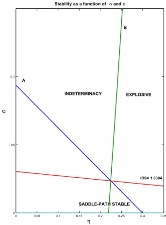
andθ(1−α) +α(1 +χ)are positive. Therefore, (13) is negative (anddet(J∗)is positive) in the region of (σ,η) space above the downward sloping straight line Ain Figure 1.
Let us turn our attention toT r(J∗) given by Ψ[−v(1− α(1−φ)
θ )−uα(1−
φ)(1−1θ)]x∗+y∗.Calculations (given in the Appendix) demonstrate that T r(J∗) = ρ(θ−1) α(1−φ)(1−1θ)× 1 α(θ−1) +χ(θ−α)−η(1 +χ)(θ−1)−σ[θ(1−α) +α(1 +χ)]× αh(1 +χ)(1−α(1θ−φ))−(1−α)(1−φ)i−(1 +χ)(1−α(1θ−φ))η+ ασh(1 +χ)(1−α(1θ−φ))−(1−α)(1−φ)i .
The term on theÞrst line is always positive, that on the second line is negative if (13) is negative, and the third line is, once again, a linear function inσ and
η.Whenσ=η= 0,the term inÞgure parentheses equals
α ·
(1 +χ)(1−α(1−φ)
θ )−(1−α)(1−φ) ¸
and is always positive as shown in the Appendix. The term inÞgure parentheses equals zero along the line Bin Figure 1, which crosses vertical axis at (0,−1)
and is upward sloping. It is positive above the lineB.
Region of the (η,σ) space generating indeterminate steady state (det(J∗)>
0, T r(J∗)<0) is the area that is at the same time below the lineσ= 1
α−1,
above line A, and above lineB.1 Line Acrosses theηaxis to the right of the
lineBfor any parameter values (see Appendix for the proof). Therefore, there exists a value of (σmin,η∗) at which indeterminacy is achieved. For smaller
values of σ the steady state is either determinate or explosive. The value of
(σmin,η∗)corresponds to a minimum degree of increasing returns to scale that
is necessary to generate indeterminate steady state, IRSmin > 1. Stability of
the steady state for smaller IRS values depends on the slope of the line A. If absolute value of this slope is greater than IRSmin, then the steady state can
be determinate or explosive. ForIRS values close to 1, only the possibility of a determinate steady state remains. If slope of Ais smaller thanIRSmin,than
the steady state forIRS < IRSmincan be indeterminate or deteminate. Again,
whenIRSis close to 1 the only outcome is determinate steady state. As is easy 1Intersection with the opposite signs – above the lineσ= 1
α−1,the lineA, and below
to see (calculation in the Appendix), absolute value of the slope of lineAis less than one for χ = 0(indivisible labor). For values of IRS slightly larger than IRSmin,one could observe all three outcomes: indeterminate, determinate, and
explosive steady state.
Notice that for some values ofη,it is possible to move from indeterminate to explosive steady state by lowering σ and decreasing the returns to scale. For large η, σ = 0 (constant returns to scale on the social level) generates explosive, rather than determinate, steady state. This behavior is similar to the one observed in the original Benhabib and Farmer (1994) model, where for β
large enough, relatively small values ofαresult in explosive steady state. Given the values of parameters determining the degree of increasing returns to scale, stability of the steady state depend on three other parameter values:χ,
θ,andφ. Notice that stability does not depend onρ, which is a usual outcome if variable capital utilization is modeled as in this paper. Stability also does not depend onΨ, one minus the symmetric equilibrium tax rate.
As demonstrated in the Appendix, increase inχ moves the points of inter-section of line A with both axes upward. Therefore, the region of the (η,σ)
space where the steady state is determinate increases. LineBrotates clockwise asχincreases, therefore increasing the region of indeterminacy at the expense of explosive region. It is impossible to say what happens to the value σmin –
the minimum degree of externality necessary for indeterminacy. Schmitt-Grohe and Uribe (1997) show that higher χ makes indeterminacy of the steady state less likely to obtain.
The steady state value of the depreciation rate is a decreasing function of the parameterθ.Usual conclusion in one—sector models is that higher depreciation rate makes indeterminacy easier to achieve, see, for example, Figure 1 in Wen (1998). In the current model, the result is not easy to predict: an increase in
θ moves the point of intersection of the lineAwithσaxis up, but intersection withηaxis decreases. LineBrotates clockwise. The effect onσminand on the
to derive analytically.
Finally, an increase inφ– higher progressivity of the tax schedule – does not inßuence lineA at all. LineBrotates clockwise around the point (0,−1). Therefore, the region of(η,σ)space where the steady state is determinate does not change, but indeterminate region increases at the expense of the explosive one. This outcome can be contrasted with Guo (1999), where more progressivity (higherφ)is stabilizing. However, in a two—sector model of Guo and Harrison (2001) progressive tax schedule can be both stabilizing and destabilizing.
4
Calibration of the tax schedule
For the calibration exersize we use the same baseline parameters values as Wen (1998):α= 0.3, χ= 0,θ= 1.4.
Calibration of the degree of progressivity of the tax scheduleφcan proceed along two paths. The Þrst way is to use IRS data on individual tax returns. The data lists average tax as a share of Adjusted Gross Income (AGI) for the returns that do claim income tax and the share of returns with no tax, see IRS (Winter 2002). Assuming that all taxpayers are located in the middle of reported income brackets, we can derive the total amount of income tax paid by the taxpayers in this income bracket. Equation (3) then gives disposable income,(1−τ)Y =ΨYφtYt1−φ orlog(DP I) =const+ (1−φ) log(Y).Assuming that AGI=Y,it is then possible to estimate parameter φ from a simple linear regression. This estimate is necessarily very imprecise, because income and AGI can differ signiÞcantly, and calculating the extent of this difference is difficult. Nevertheless, the results could be taken as a guideline for other calibration methods. For the 2000 data, this calibration method givesφfrom 0.046 (if the whole range of the data is used) to 0.066 (when data points with AGI below $3,000 and above $1,500,000 are excluded).
The second method of calibratingφis as follows. We start from an assump-tion that distribuassump-tion of income in the populaassump-tion follows a Gamma distribuassump-tion with parametersαandβ.Gamma distribution has been used to approximate the
true distribution of income among households, see Dragulescu and Yakovenko (2001) and Ferrero (2003). Gamma distribution has a non—zero mode for values ofαgreater than one, and can resemble log—normal distribution that is usually used to approximate the distribution of income.
The Gini coefficient is the area between 45◦ line and the Lorenz curve rep-resenting the distribution of income. Horizontal coordinate x(r) of this curve represents the cumulative fraction of population with income below r, and the vertical oney(r)is the share of this fraction in the total income:
x(r) = r Z 0 P(s)ds, y(r) = r R 0 sP(s)ds ∞ R 0 sP(s)ds . (14)
The Gini coefficient is then given as G= 2
1 Z 0
(x−y)dx. (15)
For details, see Dragulescu and Yakovenko (2001). If one assumes that the pre— tax income distributionP is given by a gamma distribution with parametersα
andβ,the Gini coefficient is given by Gin= 1 √πΓ(α+ 1 2) Γ(α+ 1).
Assuming the progressive tax of the form used in this paper, after—tax income of the agent with pre—tax incomeY is given by ΨYφtYt1−φ. To calculate post— tax Gini index, one then substitutesΨYφts1−φ instead ofsinto the formula for
y(r) above. The expression under the integral becomes a probability density function of a gamma distribution with differentαbut the sameβ.Calculating the integral in (15), one can show that post—tax Gini coefficient is given by
Gf in = 2· ∞ Z 0 f(r,α,1)·[F(r,α,1)−F(r,α+ 1−φ,1)]dr= (16a) 1−2· ∞ Z 0 f(r,α,1)·F(r,α+ 1−φ,1)dr (16b) = 2· ∞ Z 0 f(r,α+ 1−φ,1)·F(r,α,1)dr−1. (16c)
Heref(r,α,1)andF(r,α,1)are p.d.f and c.d.f. of the gamma distribution with parameters αand 1, respectively.
To calibrate φ, one then needs only two numbers: pre—tax and post—tax Gini coefficients. Pre—tax coefficient is used to determine α, and parameter
φ is chosen so that formulae (16) produce empirically observed post—tax Gini coefficient.
The data for this calibration method are taken from the Current Population Reports on consumer income by the US Census Bureau, see Jones and Weinberg (2000). US Census Bureau compiles data on consumer income together with sev-eral experimental measures of income, including pre—tax and post—tax income. Figure 7 in Jones and Weinberg (2000) contains Gini coefficients for pre—tax and post—tax household income from 1993 to 1998. The algorithm described above shows that the pre—tax income distribution can be approximated by the gamma distribution withαfrom 1.24 to 1.30, and the degree of progressivity of the tax,φ,varies from 0.086 to 0.103.
Direct estimation ofφrequires access to the raw USCB data for consumer income, taxes paid, and post—tax income.
For a value ofφon the upper side of our estimated range, 0.10, indeterminacy can be observed if degrees to scale on the social level are above 1.0304, or 3% increased returns to scale. This value is extremely low. If we set η equal to zero, the minimal returns to scale jumps to at least 9% (lineAintersectsσaxis slightly above 1.09, therefore indeterminacy is impossible for lower values of σ
and increasing returns to scale). On the other hand, such a low value of returns to scale is compatible with indeterminacy only if productivity of the ratio of the ßow of public spending to theßow of capital services is relatively high, 0.22. As noted in the previous section,ηadds only second—order terms to the returns to scale, but inßuences stability to theÞrst order.
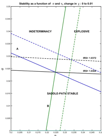
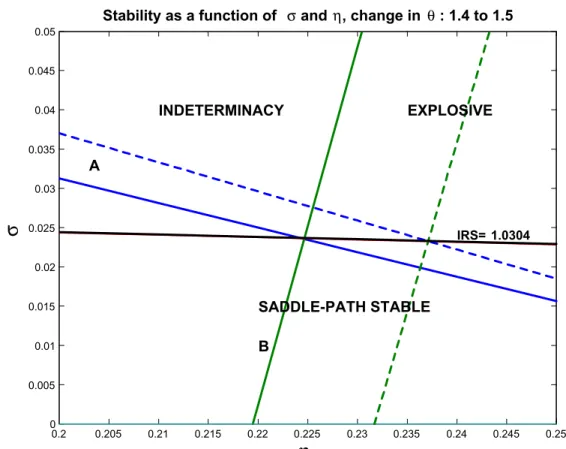
Figures 2 through 4 present the effect of changes in the basic parameters,
θ, χ, and φ, on the minimun level of increasing returns to scale necessary to generate indeterminacy. A small increase in χ reduces the area of the (η,σ)
space in which saddle—path stability is not observed and thus is stabilizing. The minimal degree of returns to scale increases slightly. This outcome is consistent with the Þndings of Schmitt-Grohe and Uribe (1997) where higher values of
χ mean that indeterminacy is less likely (one needs much higher tax rates to generate indeterminacy). Similar outcome is observed in Wen (1998).
An increase inθ (and corresponding decrease in the steady state depretia-tion rate) has similar effects: the area of the(η,σ)space in which saddle—path stability is not observed is reduced, and thus the change is stabilizing. However, there is essentially no inßuence on the minimal degree of returns to scale. Again, this result is consistent with Wen (1998), where a decrease in depretiation rate (increase in θ) lead to the decrease in the area of parameter space generating indeterminacy by requiring higher degrees of returns to scale; for the value of the depretiation rate 0.10 (this corresponds toθ= 1.4used both in Wen (1998) and here), this decrease is very small.
Finally, a reduction of φ from 0.10 to 0.08 leads to a large increase of the area of the the (η,σ)space in which steady state is explosive. Minimal degree of returns to scale necessary to generate indeterminacy increases by less than one percentage point. As explained above, the change of φ does not inßuence the area of the (η,σ) space in which saddle—path stability is obtained. This result is in direct contrast with Guo (1999), where more progressivity (higher
φ)is stabilizing. However, note that in a two—sector model of Guo and Harrison (2001) progressive tax schedule can be both stabilizing and destabilizing. In our model, an increase inφcould mean both increase and decrease in the minimal degree of returns to scale necessary to obtain indeterminacy (the result depends on the relative slopes of the line A and iso—IRS line on Figure 1; for values of χ that are high enough, line A could become less steep than the iso—IRS line, and an increase in φwill mean hgher minimal degree of IRS necessary for indeterminacy).
What can we say about the slope of the labor demand curve when parameter values imply indeterminacy, say, near the point (σmin,η∗)? Treating capital
utilization rateuas aÞxed parameter, the slope of the labor demand curve (in log—log coordinates) is given by
(1−α)(1 +σ) 1−η −1 = 1−α 1−η + (1−α) σ 1−η−1.
Remember that 1−ση = IRSmin−1 and is extremely low at (σmin,η∗). 11−−αη
could be less than one near η∗ because the line B crosses the η axis to the left of αand the line A to the right ofα,therefore η∗ could be on the either side of α. For the baseline parametrization used here, η∗ < α, see Figure 1. Therefore. the labor demand slopes downward – slope equals −0.078 for the baseline parametrization. For this parametrization, the whole area of the(η,σ)
space shown in Figures 2 through 4 generates a downward sloping labor demand curve.
5
Goodness—of—
Þ
t measures
To be written.
6
Conclusion
We combined several previously described extentions of a basic one—sector model with externalities: variable capital utilization, progressive tax schedule, and productive public spending. Variable capital utilization allows one to keep the degree of returns to scale, at which saddle—path stability of the steady state disappears, very low. It also allows one to generate indeterminate steady state with downward sloping labor demand curve. Progressive taxation was shown to favor saddle-path stability in one—sector models and to have mixed effects in two—sector model. Modeling productive government spending with elastic labor supply has not been attempted before.
Theoretical analysis of the stability conditions shows that the stability, in addition to the externality parameter σ and public expenditures exponent η, depends only on 4 parameters: capital shareα; inverse of the Frish labor sup-ply elasticity with respect to wage, χ; capital utilization parameter θ (steady
state depretiation rate is a decreasing function ofθ);and the the degree of pro-gressivity of the tax code. We were interested in mapping the (η,σ)space for values of parameters leading to saddle—path stable, indeterminate, or explosive steady state. The stability does not depend on the discount rateρ; this result seems to be common to one sector continuous—time models if the variable capital utilization rate is modeled as in Wen (1998).
The most clear results are obtained with respect toφandχ.Increased pro-gressivity of the tax schedule does not inßuence the area of the(η,σ)space in which saddle-path stability obtains; it increases the indeterminate region at the expense of the explosive one. On the other hand, increasedχ (lower elasticity of the labor supply) makes saddle—path stability easier to obtain and decreases the explosive region in the(η,σ)space. Effect ofθis impossible to qualify ana-lytically, but for the baseline parametrization used here higherθ (lower steady state depretiation rate) has an effect similar to the increase inχ.
The degree of returns to scale necessary to generate indeterminate steady state is extremely low in the model. For the baseline parametrization, it is given by 1.03 and is well within the range estimated by Basu and Fernald (1997). It is possible to obtain indeterminacy with downward sloping labor demand curve. We discussed two methods of calibrating the degree of progressivityφof the tax schedule. We attempted to use IRS data on personal income tax returns to calibrate this parameter. This approach suffers from the necessity to use Adjusted Gross Income instead of the true personal income and given values of φ in the 0.046÷0.066 interval. An alternative approach is to assume that pre—tax household income is distributed according to a gamma distribution, and calibrate parameterαof the gamma distribution andφso that pre—tax and post— tax Gini coefficients, derived from the theoretical distribution, corresponded to the ones reported in the Current Population Reports by the US Census Bureau. This approach gives a range of0.086÷0.103for the parameterφ.This approach suffers from the necessity to assume original income distribution and using only one statistics – Gini coefficients – to derive the parameters of interest. A
better usage of the US Census Bureau data might result in a more reliable estimate of the parameterφ.
A
Derivations
A.1
Values of
w, u,
and
v
w = θ(1 +χ) DEN × {ηln(1−Ψ) +α(1 +σ)−η θ ln Ψα(1−φ) θξ + (1−α) (1 +σ)−η 1 +χ ln Ψ(1−α) (1−φ) A }, (17a) v = θχ[1−α(1 +σ)]−σ DEN , (17b) u = θ(1−α) (1 +σ) DEN , (17c) DEN = (1−η)θ(1 +χ)−(α(1 +σ)−η) (1 +χ)−(1−α) (1 +σ)θ(17d).
A.2
Calculation of
T r
(
J
∗)
T r(J∗) = Ψ[−v(1−α(1−φ) θ )−uα(1−φ)(1− 1 θ)]x ∗+y∗= ρ(1− α(1−φ) θ ) α(1−φ)(1−1θ)− −[v(1−α(1−φ) θ ) +uα(1−φ)(1− 1 θ)] ρ α(1−φ)(1−1 θ) = ρ×n1−α(1θ−φ)−v(1−α(1θ−φ))−uα(1−φ)(1−1θ)o α(1−φ)(1−1 θ) = ρ×n³1−α(1θ−φ)´(1−v)−uα(1−φ)(1−1θ)o α(1−φ)(1−1θ) .First, let calculate (1−v) :
(1−η)θ(1 +χ)−(α(1 +σ)−η) (1 +χ)−(1−α) (1 +σ)θ−θχ[1−α(1 +σ)] +θσ DEN = −θη(1 +χ) +α(1 +σ)θ(1 +χ)−(1 +χ) (α(1 +σ)−η) DEN = = (1 +χ)(θ−1) (α(1 +σ)−η) DEN .
Then,T r(J∗)becomes ρ α(1−φ)(1−1θ)DEN × ½µ 1−α(1−φ) θ ¶ (1 +χ)(θ−1) (α(1 +σ)−η)−θ(1−α) (1 +σ)α(1−φ)θ−1 θ ¾ = ρ(θ−1) α(1−φ)(1−1θ)DEN × ½µ 1−α(1−φ) θ ¶ (1 +χ) (α(1 +σ)−η)−(1−α) (1 +σ)α(1−φ) ¾ = ρ(θ−1) α(1−φ)(1−1θ)DEN × αh(1 +χ)(1−α(1θ−φ))−(1−α)(1−φ)i−(1 +χ)(1−α(1θ−φ))η+ ασh(1 +χ)(1−α(1θ−φ))−(1−α)(1−φ)i .
A.3
Nonnegativity of
(1 +
χ
)(1
−
α(1θ−φ))
−
(1
−
α
)(1
−
φ
).
Rewrite (1 +χ)(1−α(1−φ) θ )−(1−α)(1−φ) (18)as1 +χ−(1−φ)£1+θχα+ 1−α¤.For largeχ the term in square parentheses could become negative turning the whole expression negative. However, notice that forχ= 0,this expression is given by
1−(1−φ) · 1−α(1−1 θ) ¸ = 1−(1−φ) + (1−φ)α(1−1 θ) = φ+ (1−φ)α(1−1 θ)>0.
Moreover, the derivative of the (18) w.r.t. χ is given by1− (1−θφ)α >0, w.r.t.
φis£1+θχα+ 1−α¤>0,and the second mixed derivative is αθ >0.Therefore, for any positive φandχ (18) is positive.
A.4
Intersections with the
η
axis.
Line B intersects theηaxis at
η = α(1 +χ)(1− α(1−φ) θ )−(1−α)(1−φ) (1 +χ)(1−α(1θ−φ)) = = α Ã 1− (1−α)(1−φ) (1 +χ)(1−α(1θ−φ)) ! <α.
Line Aintersect the ηaxis at η = α(θ−1) +χ(θ−α) (1 +χ)(θ−1) = α 1 +χ+ χ 1 +χ θ−α θ−1 > α 1 +χ+ χ 1 +χ > α+χ 1 +χ >α (becauseα < 1).
Therefore, lineA always intersect theηaxis to the right of the lineB.
A.5
Slope of line A
References
Barro, R. J., andX. Sala-I-Martin(1992): “Public Finances in Models of
Economic Growth,”Review of Economic Studies, 59, 645—661.
Basu, S., and J. G. Fernald(1997): “Returns to Scale in U.S. Production:
Estimates and Implications,”Journal of Political Economy, 105., 249—83.
Benhabib, J., and R. E. Farmer (1994): “Indeterminacy and Increasing
Returns,”Journal of Economic Theory, 63, 97—112.
Bennett, R. L., and R. E. A. Farmer (2000): “Indeterminacy with Non—
Separable Utility,”Journal of Economic Theory, 93, 118—43.
Bruha, J.(2003): “Indeterminacy and Productive Public Spending in a Simple
Open Economy Model,” CERGE-EI mimeo.
Cazzavillan, G.(1996): “Public Spending, Endogenous Growth, and
Endoge-nous Fluctuations,”Journal of Economic Theory, 71, 394—415.
Dragulescu, A. A., and V. M. Yakovenko (2001): “Exponential and
Power—Law Probability Distributions of Wealth and Income in the United Kingdom and the United States,”Physica A, 299, 213—221.
Ferrero, J. C.(2003): “The Statistical Distribution of Money and the Rate
of Money Transference,” cond-mat/0306322.
Guo, J.-T. (1999): “Multiple Equilibria and Progressive Taxation of Labor
Income,”Economics Letters, 65, 97—103.
Guo, J. T.,andS. G. Harrison(2001): “Tax Policy and Stability in a Model
with Sector-SpeciÞc Externalities,”Review of Economic Dynamics, 4, 75—89.
IRS (Winter 2002): “Statistics of Income Bulletin, Historical Table http://www.irs.gov/taxstats/article/0„Id=96981,00.html,” .
Jones, A. F., and D. H. Weinberg (2000): “The Changing Shape of the
Park, H., and A. Philippopoulos(2002): “Dynamics of Taxes, Public Ser-vices, and Endogenous Growth,”Macroeconomic Dynamics, 6, 187—201.
Schmitt-Grohe, S.,andM. Uribe(1997): “Balanced-Budget Rules,
Distor-tionary Taxes, and Aggregate Instability,”Journal of Political Economy, 105, 976—1000.
Wen, Y. (1998): “Capacity Utilization under Increasing Returns to Scale,”
Journal of Economic Theory, 81, 7—36.
Zhang, J. (2000): “Public Services, Increasing Returns, and Equilibrium
Figure 1: Stability regions in the(η,σ)space.
0 0.05 0.1 0.15 0.2 0.25 0.3 0.35 0
0.05 0.1
Stability as a function of σ and η
η σ A B IRS= 1.0304 INDETERMINACY EXPLOSIVE SADDLE-PATH STABLE
Figure 2: Stability regions change withχ. 0.2 0.205 0.21 0.215 0.22 0.225 0.23 0.235 0.24 0.245 0.25 0 0.005 0.01 0.015 0.02 0.025 0.03 0.035 0.04 0.045 0.05
Stability as a function of σ and η, change in χ : 0 to 0.01
η σ A B IRS= 1.0304 IRS= 1.0372 INDETERMINACY EXPLOSIVE SADDLE-PATH STABLE
Figure 3: Stability regions change with φ. 0.2 0.205 0.21 0.215 0.22 0.225 0.23 0.235 0.24 0.245 0.25 0 0.005 0.01 0.015 0.02 0.025 0.03 0.035 0.04 0.045 0.05
Stability as a function of σ and η, change in φ : 0.10 to 0.08
η σ A B IRS= 1.0304 IRS= 1.0378 INDETERMINACY EXPLOSIVE SADDLE-PATH STABLE
Figure 4: Stability regions change withθ. 0.2 0.205 0.21 0.215 0.22 0.225 0.23 0.235 0.24 0.245 0.25 0 0.005 0.01 0.015 0.02 0.025 0.03 0.035 0.04 0.045 0.05
Stability as a function of σ and η, change in θ : 1.4 to 1.5