The Determinants of Farmland Values in Canada

(1)

THE DETERMINANTS OF FARMLAND

VALUES IN CANADA

CATPRN Working Paper 2008-03

March 2008

Jeevika Weerahewa

Agricultural Economics and Business Management University of Peradeniya, Sri Lanka

Karl D. Meilke

Food, Agricultural and Resource Economics University of Guelph, Guelph

Richard J. Vyn

Economics and Business

University of Guelph Ridgetown Campus

Zahoor Haq

Food, Agricultural and Resource Economics University of Guelph, Guelph

http://www.catrade.org

Funding for this project was provided by the Canadian Agricultural Trade Policy Research Network (CATPRN). The CATPRN is funded by Agriculture and Agri-Food Canada but the views expressed in this paper are those of the authors and should not be attributed to the funding agency.

(2)

2 1.0 Introduction

Farmland values in Canada have increased significantly over the past 60 years and in particular since the mid-1980s (figure 1). Over the past 20 years agriculture has been characterized by productivity increases but until very recently crop prices have been stagnate or declining and hence total returns have not experienced the significant increase that would seem necessary to explain escalating land values. For example, nominal farmland values in Canada between 2000 and 2005 increased from $844 per acre to $949 per acre (12.4 percent) in spite of the fact that net farm income, excluding government payments, averaged a negative $972 million dollars annually (Statistics Canada, 2006). Only government payments that averaged $3,686 million per year over the same time period moved the sector into the black.

Figure 1: Value of Land and Buildings in Canada, $/acre, 1960-2005

0 100 200 300 400 500 600 700 800 900 1000 1960 1963 1966 1969 1972 1975 1978 1981 1984 1987 1990 1993 1996 1999 2002 2005 $ / Acre

Consolidation in the farm sector driven by economies of size and for the past ten years and generally easy credit conditions have led to increased demand for land; and with a relatively fixed land supply there has been upward pressure on prices. Still it is hard to imagine land values escalating to the extent they have without significant transfers of income from taxpayers and consumers to the agricultural sector. Farm programs, in Canada, are designed to provide income support to protect farmers from the inherent production and market risks they face. The primary objective of such programs is to provide payments that compensate farmers for lost income. However, these payments may also be capitalized into the value of assets such as land, which forces asset prices higher. If producers are using government payments to justify higher prices for land, this

(3)

3 implies that these programs are camouflaging market signals and are not fully meeting their objectives.1 The increasing land values could, in turn, lead to more demand for government payments to compensate producers for the lower incomes exacerbated by higher asset values.

There have been a number of studies undertaken to address this issue. Weersink et al. found that land values in Ontario are more responsive to government payments than to market returns. Roberts, Kirwan, and Hopkins found the incidence of government payments on land rents in the U.S. was between 34 and 41 cents for each dollar of payment. Shaik, Helmers, and Atwood also found a significant positive relationship between government payments and land values in the U.S. However, their results indicate that the share of land values generated by government payments has decreased in recent years. During the 1960’s and 1970’s, this share was as high as 40 percent, but since 1990, the share has dropped to between 15 and 20 percent.

The decline in the share of land values generated by government payments, as suggested by Shaik, Helmers, and Atwood, has coincided with a shift in government spending from “coupled” programs to “decoupled” programs. Agricultural programs are considered to be coupled if their benefits are directly related to production. Such programs can significantly influence farmers’ production decisions. For example, a price support program that compensates farmers for low commodity prices will influence their production decisions if the size of the payment is based on their current output. Conversely, if the payments are based on historical production, their influence on production decisions is minimal and the programs are often considered to be decoupled. Some program payments increase total farm revenue, but they do not increase per-unit net returns of specific production alternatives (whole farm programs), and thus do not offer incentives to increase production of one commodity over another. Of course, these payments may keep resources in agriculture that would otherwise leave the sector (USDA, 2003).

In the U.S., the 1996 Federal Agriculture Improvement and Reform (FAIR) Act implemented policy changes designed to shift government support from coupled programs to programs that would be less production and market distorting. Payments under these programs were based on historical area and yields for each producer, thus decoupling payments from current production decisions. This shift to decoupled programs occurred partly in response to the WTO negotiations, which stipulated that government payments in either the Blue Box or Green Box would not be subject to disciplines under the Uruguay Round Agreement on Agriculture (WTO, 1994)2. Under the draft text tabled by Chairman Falconer, as part of the multilateral Doha Development Agenda negotiations government payments in the blue box would be subject to international disciplines (WTO, 2008).

1_{This implies that maintaining the wealth of farmers through constant or higher farm land values is not an}

objective of government programs – an assumption that is open to serious challenge.

2_{The Blue Box and Green Box programs are defined in Article 6, section 5(a) (}_{Domestic Support}

Commitments) and Annex 2 (Domestic Support: The Basis for Exemption from the Reduction

(4)

4 This shift has occurred in Canada as well, although in Canada it can be argued that the current programs are only partially decoupled. Recent programs such as the Net Income Stabilization Account (NISA) program and the Canadian Agricultural Income Stabilization (CAIS) program focus on income support rather than price support and on whole farm coverage instead of commodity specific coverage. While these programs are no longer coupled to production decisions for specific commodities, they cannot be considered fully decoupled since compensation is still based on current output. However, this shift away from fully coupled programs may affect the impact that program payments have on farmland values.

2.0 Objectives

The primary objective of this study is to determine the impact of changes in income from the market and government payments on farmland values in the Canadian provinces. Analysis is also undertaken to see if the form of government payments has an impact on the degree to which they are capitalized into land values. The form of government payments is proxied by separating the sample period, 1959-2004, into three general policy regimes: 1) 1959-1974 when government payments were minimal and commodity specific; 2) 1975-1990 when government payments were generally commodity specific and rising rapidly; and 3) 1991 to 2004 when government payments were generally non-commodity specific3. In addition, the elimination of the Western Grain Transportation Rate subsidy in 1995 represented an abrupt and permanent change in government policy that would be expected to change producers forecasts of future returns from grain production in the affected provinces. If the form of government payments matters, then this should be taken into account in designing farm policies.

How agricultural policy affects land values and how the benefits of government programs are distributed have important policy implications. When land prices increase as a result of the capitalization of government payments, production costs increase, and the benefits are transferred from the producer to the land owner. A study by Kuchler and Tegene suggests that because the supply of agricultural land is relatively fixed, program payments accrue only to the land owner. One important feature of modern farming is the increasing “disconnect” between agricultural production and land ownership4. Consequently, even though payments are often made directly to the producer, the land owner will often reap the benefits of the program through higher land rents. In this case, producers can benefit from government payments only if they are also the land owners. However, if the rate of capitalization of government payments into land values is decreasing, this would imply that more of the benefits remain with producers instead of being passed on to landowners.

3_{There are, of course, exceptions to this general characterization of farm programs during these time}

periods, however we feel it is a good characterization of federal safety-net programs.

4_{In the United States 43.7 percent of land operated by farms is rented (USDA, 2005). In Canada, the}

(5)

5 Another factor that may play a major role in determining land values, particularly in more populated regions, is the influence of urban growth. With a constantly increasing population in major urban areas, the growth of cities continues to encroach on valuable agricultural land. Land that is sold for development commands a large premium, and as cities expand, surrounding agricultural land may be purchased speculatively at prices that far exceed expected returns from agricultural production. To account for this influence, population factors are incorporated into the framework used in this study.

The next section reviews the general approach to valuing land and discusses a number of studies that have used, extended, or revised this approach. Results of previous studies are also discussed in this section. In the following section, an empirical framework is developed for estimating the effects of government payments on land values across Canada. An overview of the empirical results is then provided. The final section offers some conclusions and suggestions for further research.

3.0 Conceptual Framework

Factors that play a role in determining farmland values have been studied for many years. Some early studies reached a number of conclusions regarding the determinants of land values and the factors that have caused changes in these values over time. Tweeten and Martin found the determinants included farm expansion pressures and capitalized government payments. Reynolds and Timmons found that land prices were determined by expected capital gains, government payments, farm enlargement, and the return on common stock. Klinefelter found that changes in land prices were explained by net returns, average farm size, number of transfers, and expected capital gains. Castle and Hoch found that land prices were determined by expected capitalized rent and expected capital gains.

The general approach to pricing assets such as farmland has been through the present value model, which involves the determination of a net present value (NPV) of the asset. This model has been used in a large number of studies to assess the determinants of land values. Burt and Alston were among the first to use the capitalization model in the context of farmland values. Others have followed, incorporating minor changes to the basic model.

The NPV is calculated by estimating the future stream of cash returns resulting from ownership of the asset, and discounting this cash flow based on the level of uncertainty inherent in the expected returns. The capitalization model derived through this approach is summarized by the following equation:

(

)

∑

∞ = + + + = 0 1 j t j j t t t _r R E V (1)

where Vt is the value of the asset, Rt is the real return from the asset based on expectations in period t (Et), and rt is the real discount rate, which may vary over time. This equation

(6)

6 can be further simplified, by assuming a constant discount rate (r) and constant returns (R ), so that:

r R

V_t = (2)

This equation has formed the basis for many studies of asset values, and has been incorporated into studies of farmland values.

The impact of farm policy on land values has been the subject of a number of studies in recent years. Most studies of the effects of government payments on farmland values attempt to measure this impact directly, usually through the capitalization model, where land values are determined primarily through expected future cash flows from the land (Weersink et al.). This model is derived from the capitalization model given in equation (1), and can be summarized as follows:

∑

∞ = + = 1 j t t j j t b E R L (3)

where Lt is the value of land, Rt is the rent from land at time t, Et is the expectations operator, and b is the discount rate, such that b = 1/(1+r).

To account for returns from both production (P) and from government payments (G), Weersink et al. expanded this model to:

∑

∞ = + + + = 1 1 2 ) ( j t t j j j t t j t b E P b EG L (4)

where b1 and b2 are the time-varying discount rates of P and G, respectively.

The value of land is thus calculated as the present value of the expected future returns, discounted according to the risk of income from each source. The discount rates from each source are allowed to differ to reflect varying levels of uncertainty associated with the different sources of future returns. The discount rate for each source of income may vary over time. However, if the discount rate for each source of income is assumed to be constant over time, then equation (4) can be simplified to:

1 2 1 1 + + + = _t _t _t _t t E P EG L β β (5)

where β1 and β2 are the respective constant discount rates for expected cash flows from production and government payments. This equation constitutes the general form for models that have previously been used for agricultural asset value determination.

3.1 Effect of Government Payments on Land Values

Empirical studies of the effect of government payments on land values have involved a number of different approaches, and have produced mixed results. Moss, Shonkwiler, and Reynolds used a vector autoregression framework to determine the relationship between farm asset values and government payments. Farm income was split into two components – market income and government payments. The authors hypothesized that the effects on real asset values of government payments would be different from those of market

(7)

7 income, as the uncertainty underlying government programs may cause these payments may be seen as transient income. The impulse response functions generated by their model showed that while increases in market income were quickly capitalized into asset values, the same did not hold true for government payments. In fact, the authors found that in the long run, increases in payments had little effect on asset values.

Goodwin and Ortalo-Magne attempted to evaluate the impact of agricultural policy reform on farmland prices. In their study, the authors used a variation on the general approach to valuing farmland, where land prices are a function of expectations of government support, farm prices, and yields. A generalized method of moments (GMM) estimator was utilized to evaluate these relationships. The results of this study indicated that a one percent change in government payments resulted in a 0.38 percent change in land prices. Returns to land through government payments were discounted significantly compared to returns based on prices and yields. This may be a result of uncertainty with respect to future government payments.

Clark, Klein, and Thompson used the present value approach to determine whether government payments were capitalized into Saskatchewan land values. In their model, land values are based on discounted expected future returns to land, which is composed of revenue from production and subsidies. The authors suggest that their land values series and returns series are correlated and that each contains a unit root. Some evidence was found that land values and income plus subsidies were cointegrated. The results of the model provided some indication that short-run subsidies were capitalized into land values.

Barnard et al. measured the extent to which government payments are capitalized into U.S. land values. This study utilized micro level data from regions across the U.S. Two different approaches were used to analyze the impact of government payments, ordinary least squares (OLS) and a non-parametric estimator. The models accounted for population influences, productivity factors, farm size, and county recreational activity. The results indicated significant spatial variability in the rate of capitalization of government payments. While the highest degree of capitalization of government payments was 50 percent, many areas had capitalization rates of 10-20 percent. The results also indicated that elimination of government payments would reduce land values from 12 to 69 percent.

Weersink et al. estimated the separate effects of market returns and government payments on farmland values in Ontario and examined the discount rates associated with each source of income. The authors modified the traditional capitalization model to allow for an examination of the two sources of income. The discount rate was allowed to vary between the two sources, allowing for the testing of the hypothesis that income from government payments is discounted more heavily than income from market returns. The system of equations was estimated using the non-linear seemingly unrelated regression technique. The authors found that returns from government payments were discounted less than returns from production, contrary to what was hypothesized. This implies that government payments have been a less risky source of income than market returns. The

(8)

8 elasticity of land values to government payments was significantly higher than that of market returns, implying that land values are more responsive to government payments. Goodwin, Mishra, and Ortalo-Magne took the standard approach, as described in equation (4), one step further. Instead of combining all government payments into one variable, they differentiated between four types of programs. This was done to account for the varying uncertainty about the future of each type of program and the expected future payments from each type of program. The results confirmed the hypothesis that different programs have different effects on land values. While payments under most types of programs had positive impacts on land values, these effects varied across year, crop, and region.

Instead of focusing on the relationship between government payments and land values, Roberts, Kirwan, and Hopkins focused on the relationship between payments and cash rents. A measure of the incidence of government payments on rents could indicate how payments are distributed between farmers and landowners. Focusing the analysis on cash rents rather than land values allowed for a greater focus on current expectations. Also, any non-agricultural influences that affect land values would not factor into the determination of land rents. The estimates derived from this analysis implied an incidence of government payments on land rents of between 34 and 41 cents for each dollar of payment. The authors suggested that the long-run incidence may be larger than was reflected in the estimates, as it may take time for rental rates to reflect changes in expected government payments. They also postulated that a larger portion of government payments may be captured by other inputs such as human capital and machinery. However, it is difficult to compare the incidence estimates from this analysis with those of other studies in which the analysis focused on land values instead of land rents.

Barnard et al. used cross-section data to analyze farmland values in the regions of the U.S. which received the largest program payments. Their approach also took into account other factors, such as soil quality, availability of irrigation, and urban influences. This analysis was used to estimate the percentage of the total farmland value that was attributable to government payments. The results indicated that program payments had the greatest impact on land values in the Heartland, where payments accounted for 24 percent of farmland value. Similar effects were found in the Prairie Gateway region (23 percent) and the Northern Great Plains (22 percent).

Other studies have found different results. Gardner, following the approach of Barnard et al., used data from 315 counties across the US to estimate the impact of government payments on land values. Recognizing the limitations inherent in using a cross-section approach, he incorporated a time series element. He found that there was only weak evidence to support the claim that government payments have caused a significant increase in land prices.

Similarly, Just and Miranowski found that government payments are only a minor factor in the determination of land prices, and that changes in government payments would often only offset changes in market returns. While government payments accounted for

(9)

9 between 15 and 25 percent of the capitalized value of land, they only accounted for a very small part of land price fluctuations. Their results suggest that inflation and the opportunity cost of capital play an important role in causing changes in land prices. The use of the capitalization model in studies of farmland values is based on the assumption of a direct and positive correlation between expected cash flows and market prices of land. However, there has been a divergence between farmland values and returns to land from agriculture. Market prices of land have increased significantly over the past decade, while there has been little increase in the cash flow generated from farmland. This has brought into question the validity of using the capitalization model in its current form. Studies began to focus on explanations that extended beyond factors directly related to agriculture.

Researchers recognized that farmland can derive additional value from the option of being converted into alternative uses. Non-agricultural uses are often more profitable, and this will cause the market value of land to be higher than the agricultural use value, with this difference being greater the closer the land is to an urban area. To purchase farmland for non-agricultural purposes, a premium must be paid to bid land away from other agricultural producers. This tends to increase the value of all land in the area, as the sale information will affect expectations of local landowners. Thus, in regions where urban pressures are stronger or where the role of agriculture has been diminished, explanatory variables accounting for urban influences should be incorporated into land value models. Shi, Phipps, and Colyer, using a pooled time-series and cross-section model, found that land values in West Virginia were influenced by the degree of urbanization. They determined that land values were inversely related to the distance from major urban centres, and directly related to the population of the urban centres. The impact of urban influences raised the price of land above its agricultural value.

Hardie, Narayan, and Gardner attempted to explain farmland prices in terms of returns from production as well as potential farm value. Their study incorporated non-agricultural factors such as house values, income, and a population index. Elasticities were calculated to show the response in farmland to changes in each of the factors. The results indicated that the elasticity of response in land prices to changes in house values decreased as the counties become more populated, while the response of land prices to changes in house values was elastic in rural counties but became inelastic in urban counties. Overall, the authors found that, while the effects of both returns from agriculture and non-farm factors were significant, farmland values were more responsive to the non-farm factors than to returns from production and from government payments. They also found that capitalization of farm revenues into land prices does not change with urbanization.

Goodwin, Mishra, and Ortalo-Magne, in addition to evaluating the impacts of specific government programs on the value of land, also accounted for the value of farmland that is derived from the option of being converted to non-agricultural uses. They included in their model indicators of urban pressure such as population density, population growth

(10)

10 rates, and the value of housing permits issued in the county. These variables were determined to have a significant impact on agricultural land values. While urban pressures significantly increased land values, these factors did not appear to affect the estimates of the other determinants.

3.2 Concerns with the Present Value Model

Some controversy exists regarding the validity of present value models for assets such as farmland. Featherstone and Baker point out that many of the early studies on land values used static models, which assume that prices instantly adjust to long run equilibrium. They attempted to account for this limitation by looking at the time path of adjustment for variables such as returns and interest rates. They also allow for the possibility of deviations from the long run equilibrium due to behaviour that is not fully rational. To conduct this study, a vector autoregression system of equations was used, where all of the variables are treated as endogenous, as each variable in the system impacts all other variables through lagged effects. The authors found that net rents cannot explain all of land price changes, as speculative forces may also play a role in land price determination. They concluded that the response of land prices to changes in expected future returns is too large and drawn out to be consistent with the present value model.

Campbell and Shiller used a cointegrated vector autoregression (VAR) model to address the problem of nonstationarity in time series that often occurs with the present value model. They developed a test of the present value model that is valid when the variables are stationary. The authors derive a method of assessing the significance of deviations from the present value model by comparing the forecast of the present value of future returns with an unrestricted VAR forecast. A new variable is defined and called the “spread” – the difference between the price of the asset and the return on asset, such that:

St = Yt - θyt,

where St is the spread, Yt is the price of the asset in period t, and yt is the return on the asset in period t.

The use of this equation helps resolve the stationarity issue, for if Δyt is stationary, then St will be stationary, which implies that ΔYt is also stationary. The VAR framework can be used to conduct statistical tests of the present value model and also to evaluate its failures. If the present value model is valid, differences between the spread St and the theoretical spread S’t should only be due to sampling error. Large differences imply economically significant deviations from the model.

Falk used the approach developed by Engel and Granger to test the validity of using the present value model for evaluating the determinants of farmland prices. He began by assuming that the present value model provided an accurate representation of the correlation between land prices and net returns. Because the real net rent time series tended to increase over time, he stated that this series was non-stationary in its mean.

(11)

11 There are two approaches that can be used to account for non-stationarity. In one approach, the series is assumed to be stationary around a linear trend. Another approach is to assume that the process is difference stationary, where the first differences of the process form a stationary process. One important difference between the two is that an unexpected change in the trend stationary approach has only a temporary effect on the process while a permanent effect results from such a change in the difference stationary approach.

Falk assumed a difference stationary process for net rents, which meant that land prices will also be difference stationary. Similar to Campbell and Shiller, Falk defined a new variable as the spread between land prices and discounted net rents. By the present value model, the spread represents the rational forecast of the present value of future changes in net rents. Past values of the spread can be used to forecast future changes in rents.

Falk then used time series data from Iowa to test whether the behaviour of land prices fits within the predictions of the present value model. He first tested whether land prices and rents were difference stationary as opposed to trend stationary. Dickey-Fuller test results indicated that the null hypothesis of difference stationarity could not be rejected. He then tested the restrictions that the present value model imposes on the VAR representation of the change in net rents and the spread. Because the restrictions were rejected, the validity of the present value model could not be supported. Though correlation existed between land prices and rents, changes in land prices were much more volatile than changes in rents. Falk suggested that the failure of the model may be due to the presence of asset bubbles, often a result of self-fulfilling beliefs regarding future movements in values. Goodwin, Mishra, and Ortalo-Magne pointed out that empirical models based on the present value model possess a fundamental limitation. Land values are based on expectations of future returns from production and from government payments; however, these expected future cash flows cannot be observed. While these expectations should be fairly stable for a given location and policy set, actual returns from both production and government programs tend to be quite variable. Thus, observations from a particular year may not be an appropriate indicator of the level of returns that can be expected in the future. The use of such observations may result in an inaccurate depiction of the magnitude of land value determinants. However, an alternative methodology was not proposed to avoid this limitation.

3.3 Challenges in Determining the Effect of Government Payments

Goodwin, Mishra, and Ortalo-Magne also identified problems that complicate empirical analysis when government payments are incorporated into the model. By considering government payments as an explanatory variable separate from market returns, there may be the problem of multiple variables observed with error. When observing payments from multiple programs, these errors could be correlated. There may also be correlation across a pooled sample of farms, as realized returns for all farms are often dependent on an aggregate set of market and policy conditions. With realized returns from government programs highly variable, there may be significant differences in the effects of policies

(12)

12 from year to year. In addition, the omission of other factors that impact land values (non-agricultural factors) may bias estimates of empirical models.

Roberts, Kirwan, and Hopkins identified other issues associated with the use of both government payments and market returns as explanatory variables. These variables tend to be highly variable relative to land values. In addition, government payments and market returns tend to be negatively correlated. In years when market returns are low, government payments will generally increase as a result. Conversely, high market returns tend to reduce the need for government payments.

The counter-cyclical nature of government payments was addressed in a study by Shaik, Helmers, and Atwood. While both expected crop returns and expected government payments were hypothesized to be positively related to land values, the inverse short-run relationship that often exists between these two variables could cause an identification issue. In an attempt to overcome this problem, the authors used a simultaneous equation model. This model contained two equations. The first equation estimated land values as a function of crop returns, government payments, and other factors. The second equation estimated government payments as a function of crop returns, the current Farm Bill, and other factors. The joint estimation of these two equations helped to overcome the identification issue. The authors suggested that this model could provide a more accurate estimation of the capitalization model.

Shaik, Helmers and Atwood’s results from the traditional single equation model indicated a negative relationship between government payments and land values, but when using the simultaneous equation capitalization model a significant positive relationship between U.S. land values and both crop returns and government payments was found. These results also suggest that land values are more responsive to crop returns than to government payments, contrary to the findings of Weersink et al. for land values in Ontario.

Shaik, Helmers, and Atwood also estimated elasticities of the crops return and government payment variables from the simultaneous equation model in order to estimate the share of land values generated by crop returns and by government payments. They tested for changes in these shares over time, with the time periods corresponding to specific farm bills that were in effect in the U.S. The authors found that the share of land values generated by government payments was as much as 40 percent before 1980. However, since 1990, this share has declined to between 15 and 20 percent. This suggests that the rate of capitalization of government payments into land values has decreased in recent years.

3.4 Summary of Literature

Overall, the literature does not present conclusive evidence as to the most accurate method for determining farmland values. The divergence between the present value of

(13)

13 future cash flows and the market price of farmland suggests that other factors beyond returns from agriculture must play a role in determining land values. Unfortunately, there is no way to avoid using unobservable data to ascertain expected future cash flows. The present value model can be questioned unless steps are taken to account for issues such as data non-stationarity. In addition, the inverse relationship between market returns and government payments may affect the significance of the impacts of each of these variables on land values. This study takes these issues into consideration in the development of a model that can be used to evaluate the determinants of agricultural land values.

4.0 Empirical Model

A simultaneous equation model is utilized in this study following Shaik, Helmers, and Atwood5. The approach begins with the traditional capitalization model, where land values are a function of net farm income and government payments. In addition, population density, real interest rates and dummy variables representing different provinces and different policy regimes are included in the pooled cross-section time-series estimation. The model is represented by:

t MB SK AL BC j j j i i i t t t t t WGTA WGTA WGTA WGTA DT DP T Rate Pop GP NFI LV ε α α α α δ β α α α α α α + + + + + + + + + + + + =

∑

9 8 7 6 5 4 3 2 1 0 _{, (6)} i=1,…,8; j=1,2; t=1,…,46.

where LV is deflated farmland value per acre, NFI is adjusted deflated net farm income per acre, GP is deflated government payments per acre, Pop is the population density (people per arable acre), Rate is the real interest rate, and T represents a linear time trend.

DP represents the provincial dummy variables, Ontario being the base province, and DT

are time period dummy variables used to capture different policy regimes: the first period (1959-1974) when government payments were largely coupled to output but minimal; the second period (1975-1990) when government payments were generally commodity specific; and the third period (1991-2004) when government payments were largely non-commodity specific and hence partially decoupled. The first period is considered the base period. The WGTA variables capture the effect of eliminating transportation subsidies (Crow Rate) provided to grain moving from Alberta (WGTAAL), Saskatchewan (WGTASK), Manitoba (WGTAMB) and parts of British Columbia (WGTABC) to export positions. The WGTA variables all equal zero for 1959 to 1994 and one for 1995 to 2004. Adjusted net farm income and government payments are expected to have a positive relationship with farmland values. The coefficient α1 shows the change in farmland value

5_{They specify farmland value as a function of expected crop returns, expected farm program payments,}

real interest rate, expected variability associated with returns, urban expansion and non-farm employment; while government payments are specified as a function of crop returns, risk, farm size, herfindahl index (to show crop diversification) and farm bill dummy variables.

(14)

14 per acre due to a unit rise in adjusted net farm income per acre and the coefficient α2 shows the change in farmland value due to a unit rise in government payments per acre. However, there may be identification issues that arise due to the inverse relationship that often exists between adjusted net farm income and government payments. Government payments tend to be higher in years when adjusted net farm income has declined, as greater payments are triggered from support programs to compensate for decreased production or market returns. This issue can be addressed by specifying a second equation that accounts for this inverse relationship. This equation estimates government payments per acre, with adjusted net farm income per acre included as an explanatory variable. t j j j i i i t t NFI T DP DT GP =α' +α' ( )0.5+α'₂ +

∑

β' +

∑

δ +ε 1 0 , (7) i=1,…,8; j=1,2; t=1,…,46.

Note that in the above equation, the square root of NFI is used in order to capture the non-linear relationship between NFI and GP. The change in government payments due to a unit rise in NFI is given by the following equation:

5 . 0 ' 1( ) 5 . 0 / ₌ − t t t dNFI NFI dGP α (8)

A negative coefficient for α’1 indicates that when NFI rises, government payments diminish. The rate of change of government payments due to a unit change in NFI is given by: 5 . 1 ' 1 ( ) 5 . 0 5 . 0 / ) /

(dGPt dNFIt dNFIt =− ⋅ ⋅ ⋅ NFIt −

d α (9)

When α’1 is negative, the above expression implies that government payments decrease at a decreasing rate (i.e., the curve is convex to the origin) suggesting that the rate of change of government payments is higher at lower levels of NFI.

Combining equations (6) and (7), the overall change in land values due to a unit change in NFI is given by:

) ) ( 5 . 0 ( / ' 0.5 1 2 1 − ⋅ ⋅ ⋅ + = _t t NFI dNFI dLV α α α (10)

Equations (6) and (7) can be estimated simultaneously to obtain the coefficients of (6) and (7) and to calculate the change in farmland values due to a unit rise in NFI as given in (10).

5.0 The Data

This study uses provincial data from 1959 to 2004 for land prices, adjusted net farm income per acre, government payments per acre, population density and real interest rates (Statistics Canada, 2006). In calculating adjusted net farm income, government payments

(15)

15 were removed from net farm income to avoid the double-counting of this revenue. Net farm income, as calculated by Statistics Canada, was further adjusted by removing land rental expenses, as these expenses are not relevant when considering land ownership, and by removing depreciation expenses, to eliminate the effects of imputed costs. Figure 2 shows the relationship between the adjusted and unadjusted net farm income series. Land prices, adjusted net farm income per acre, and government payments per acre were deflated by the gross domestic product (GDP) deflator (1997 = 100). Provincial population figures were divided by the amount of arable land to determine population density. A real interest rate is calculated by adjusting the chartered bank prime business lending rate, for inflation, as measured by the GDP deflator.

Figure 2: Adjusted Net Farm Income and Unadjusted Net Farm Income, Constant 1997$/acre, 1959-2004 -20 -10 0 10 20 30 40 50 60 70 80 90 1959 1962 1965 1968 1971 1974 1977 1980 1983 1986 1989 1992 1995 1998 2001 2004 $ / A cr e

(16)

16 Figure 3: Adjusted Net Farm Income and Government Payments, Constant 1997$/acre, 1959-2004 0 20 40 60 80 100 120 1959 1962 1965 1968 1971 1974 1977 1980 1983 1986 1989 1992 1995 1998 2001 2004 $/ acre

Net Farm Income Government Payments

5.1 Statistical Properties of the Data

Table 1 shows the descriptive statistics for deflated farmland values per acre, adjusted deflated net farm income per acre (constant 1997 dollars) and deflated government payments per acre in six of the nine provinces included in the analysis, by time period, and figure 3 shows the trends in adjusted net farm income and government payments per acre, in Canada, between 1959 and 2004. The key data for all of the provinces are presented in table 2 and Appendix figures 1A to 9A.

(17)

17 Table 1: Land Values, Adjusted Net Farm Income and Government Payments for Selected Provinces (constant 1997 dollars/acre).

Province Time Period

1959-1974 1975-1990 1991-2004

constant 1997 dollars per acre Alberta

Land value 292 665 592

Adjusted net farm income 40 30 21

Government payments 2 8 11

British Columbia

Land value 778 1,417 1,800

Nova Scotia

Ontario

Land value 1,122 2,261 2,617

Quebec

Land value 478 922 1,405

Saskatchewan

It is clear from table 2 that the average (1959-2004) farmland values are highest in Ontario ($1973/acre) followed by British Columbia ($1311/acre). The lowest average land value is in Saskatchewan ($335/acre). Ontario also has the highest mean value for adjusted net farm income ($49.14/acre) among the provinces. Quebec ranks second ($46.45/acre) and Alberta has the lowest adjusted net farm income ($11.32/acre). The highest mean value for government payments is in Quebec ($40.23/acre), followed by PEI ($21.98/acre) and Ontario ($18.22/acre). Government payments in the other provinces are fairly uniform ranging from $7.03/acre in Alberta to $9.13/acre in New Brunswick. Table 1 shows for the six provinces illustrated that average farmland values

(18)

18

Table 2: Descriptive Statistics for Farmland Values, Adjusted Net Farm Income and Government Payments, by Province, 1959-2004 average.

PEI NS NB QU ON MB SK AB BC

Farmland Values (constant 1997 dollars/acre)

Mean 970.32 701.13 584.15 914.55 1973.30 414.19 335.78 513.01 1311.45 Std Deviation 475.51 293.55 256.50 422.22 716.53 112.23 120.01 210.73 483.10 Minimum 323.31 230.05 230.05 404.14 764.92 217.61 161.65 198.96 603.35 Maximum 1761.11 1083.49 1041.24 1816.33 2909.33 682.20 635.61 1003.69 2018.07 CV 49.01 41.87 43.91 46.17 36.31 27.10 35.74 41.08 36.84

Adjusted Net Farm Income (constant 1997 dollars/acre)

Mean 43.11 33.83 34.41 46.45 49.14 17.83 14.36 11.32 23.57 Std Deviation 58.56 20.43 27.44 27.78 43.48 19.80 20.07 15.98 26.69 Minimum -168.47 -20.48 -47.32 -25.98 -30.83 -20.63 -22.45 -20.98 -22.65 Maximum 195.92 73.18 128.63 86.12 138.14 62.96 59.02 39.84 73.45 CV 135.82 60.39 79.75 59.80 88.48 111.06 139.81 141.19 113.25

Government Payments (constant 1997 dollars/acre)

Mean 21.98 7.86 9.13 40.23 18.22 8.83 7.31 7.03 8.83 Std Deviation 16.68 5.99 7.40 26.07 13.87 8.13 7.04 6.66 7.81 Minimum 0.09 0.09 0.07 0.07 0.08 0.64 0.15 0.55 0.11 Maximum 84.92 22.46 34.17 94.65 53.93 31.65 25.39 23.79 26.07 CV 75.92 76.23 81.11 64.81 76.10 92.17 96.33 94.70 88.50 PEI: Prince Edwards Islands, NS: Nova Scotia, NB: New Brunswick, QU: Quebec, ON: Ontario, MB: Manitoba, SK: Saskatchewan, AB: Alberta, BC: British Columbia.

(19)

19

increase across the three time periods in all provinces except Alberta and Saskatchewan where they decline from the second to the third time period.

Appendix Figures 1A to 9A show a steady increase in real farmland values, in all provinces, from 1959 to 1980. With the exception of PEI, Nova Scotia and New Brunswick, a sharp drop in real farmland values began in the early-1980’s and lasted for most of the decade. Over the past 15 years real land values have generally risen everywhere. While adjusted real net farm income per acre shows significant fluctuations (the coefficient of variation ranges from 60 percent in Nova Scotia and Quebec to 140 percent in Alberta and Saskatchewan), the values of government payments per acre seem to be rising and exhibiting more stability (the coefficient of variation ranges from 65 percent in Quebec to 96 percent in Saskatchewan).

5.2 Tests for Unit Roots

The estimation of equations (6) and (7) using conventional econometric techniques are valid only if the underlying time series do not contain unit roots, i.e., they are stationary (denoted as I(0)). In the presence of unit roots, conventional econometric techniques can produce spurious estimates as the error terms are correlated. In many cases, even though the time series are non-stationary in their level form, they are stationary in first difference form. In this context, the time series is integrated of order one, denoted as I(1).

Even if the individual time series are non-stationary, i.e., I(1), certain linear combinations of these series could be stationary, i.e., I(0). If that is the case, the variables are said to be cointegrated and they obey an equilibrium relationship in the long run, although they may diverge substantially from the equilibrium in the short run. Testing for cointegration can be done by checking whether the residuals of the econometric model are stationary, I(0). Unit root tests were conducted for each of the data series, by province, and for the residuals in equations (6) and (7) using the Dicky-Fuller test. In particular, the following approach was used. The first differences of each data series were calculated and then regressed on the lagged dependent variable, one year lagged level variable and a time trend. A statistically significant coefficient for the lagged level variable (λ2), in equation (11), confirms the non-existence of unit roots, i.e., the series is stationary.

t t t t Y Y time Y =λ +λ Δ +λ +λ +ε Δ ₀ ₁ ₋₁ ₂ ₋₁ ₃ , (11)

where Y is the value of the series considered and ΔYt is Yt-Yt-1.

The results of the Dickey-Fuller tests are provided in table 3 and they indicate that the existence of unit roots in approximately one-half of the series could not be rejected6. Furthermore, a clear pattern could not be observed among different series and different provinces. Next, the same tests were performed on the data in first-difference form. The bulk of the first-differenced data is stationary and consequently, cointegration models

6_{Further tests on stationarity indicate that the first differences of most of the series do not contain unit}

(20)

20 Table 3: Dicky Fuller Test Results*

PEI NS NB QU ON MB SK AB BC Levels Farmland values -2.55 -1.34 -2.29 -3.33 -3.31 -2.41 -2.41 -3.26 -2.76 Payments -4.85 -3.54 -3.91 -3.78 -3.87 -3.06 -2.52 -2.42 -2.48 NFI -5.04 -2.83 -4.17 -3.76 -3.01 -3.39 -3.36 -3.05 -2.47 Rate -1.83 -1.83 -1.88 -1.83 -1.83 -1.83 -1.83 -1.83 -1.83 Population -0.49 -0.96 -0.63 -1.32 -3.66 -2.50 -2.42 -2.69 -2.43 First differences Farmland values -3.93 -3.24 -4.07 -3.43 -2.50 -3.11 -2.34 -3.55 -3.20 Payments -6.77 -8.79 -7.28 -9.28 -6.32 -4.91 -4.32 -4.54 -4.29 NFI -6.23 -9.38 -6.21 -8.44 -7.62 -6.34 -6.66 -5.10 -5.85 Rate -6.08 -6.08 -6.08 -5.94 -6.08 -6.08 -3.30 -6.08 -6.08 Population -2.62 -3.65 -4.08 -3.07 -3.18 -4.29 -3.21 -2.95 -3.11

*The numbers show the calculated τ statistic for the coefficient in the lagged level variable in each series. The critical τ values are -3.96 at 1% level, -3.41 for 5% level and -3.13% for 10% level.

PEI: Prince Edwards Islands, NS: Nova Scotia, NB: New Brunswick, QU: Quebec, ON: Ontario, MB: Manitoba, SK: Saskatchewan, AB: Alberta, BC: British Columbia.

(21)

21

were estimated expecting that there is a long-run relationship among variables. Equations (6) and (7) were then estimated simultaneously in level form, as in a conventional regression model, using seemingly unrelated regression, and then the residuals of the each equation were tested to see if unit roots exist.

6.0 Results of Econometric Estimation

Table 4 shows the key results for the co-integration tests for the two equations.7_They indicate that both residual series have co-integrated vectors. As a result, equations (6) and (7) contain long-run equilibrium relationships.

Table 4: Co-integration Estimation Results on the Residuals Dependent

Variable Independent Variables Coefficient τ statistic Farmland

value

Constant -1.31 Lagged dependent variable -0.11 -6.18***

Lagged first difference 0.40

Time trend 0.04

Government payments

Constant -0.48 Lagged dependent variable -0.30 -7.17***

Lagged first difference -0.04

Time trend 0.02

*** Statistically significant at 1% level. The critical value for the farmland value equation (m=5) is -5.25 and for the government payment equation is (m=2) -4.32.

Equations (6) and (7) were estimated simultaneously for the period 1959-2004 using seemingly unrelated regression (SUR). Different variants of the model were estimated and some of the results are sensitive to the exact specification of the model. We only present the results for the entire sample period (1959-2004) and for two specifications that are sufficient to illustrate representative results.

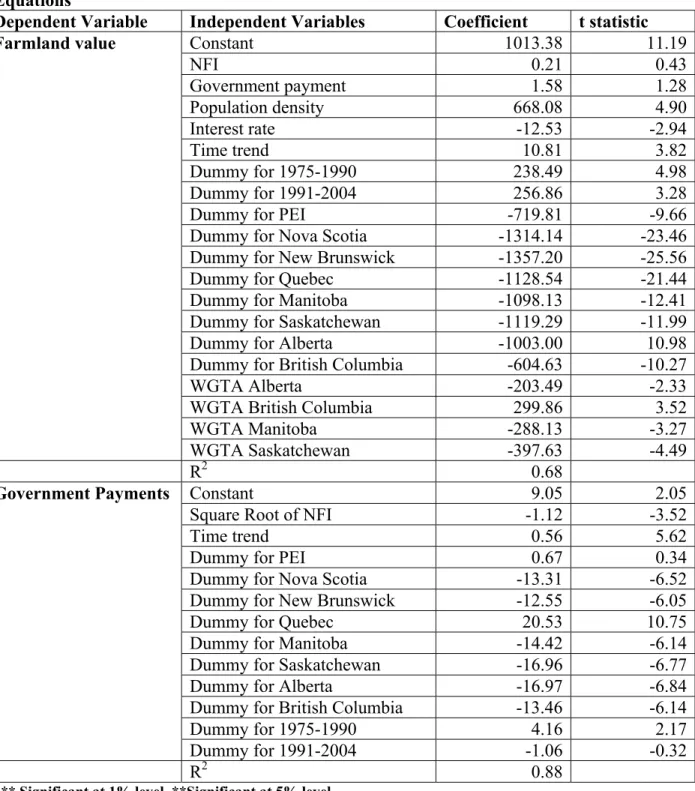
Table 5 shows the detailed results of the SUR estimates of equations (6) and (7). As expected, the effects of adjusted net farm income and government payments on farmland values are positive but the t-values on both of the estimated coefficients are small. Even a joint test that the coefficients for both adjusted farm income and government payments are zero is not rejected at a probability level of 20 percent. Further, the results show that the time trend variable has a positive coefficient indicating that farm land values have a secular trend of $10.81/acre over the sample period.

7_{After the adjustment to net farm income discussed in section 5.0 four of the 414 values for adjusted net}

farm income are negative. These negative values create problems because in equation (7) we take the square root of adjusted net farm income. Obviously, that is impossible if the value is negative. In the results that follow the year and province in which these negative values occur are dropped from the sample period. Some experimentation with alternative specifications that retain the four negative values strongly suggests that their elimination has no effect on our conclusions.

(22)

22

In table 6, the time trend variable is dropped from the estimation and it has a major effect on the coefficient for government payments, which increases from 1.58 in table 5 to 3.75 (with a t-statistic of 3.07) in table 6. Deleting the time trend variable changes the coefficient estimates for all of the other explanatory variables but in economically meaningless ways, including the coefficient on adjusted net farm income that remains small and insignificant. However, using the specification in table 6, the joint test that the coefficients on adjusted net farm income and government payments are both zero is rejected with a t-value of 2.81. Given the differences in the results in table 5 and table 6 what can we say? First, the seeming disconnect between adjusted net farm income and land values observed from casual observation of the data is confirmed by the statistical analysis. Second, government payments have been increasing over time making them difficult to disentangle from a secular trend. This is clear from the coefficient on the time trend variable in equation (7) that shows government payments increasing $0.56/acre/year, certeris parabis. As a result, the analyst is left with concluding either that: 1) farm land values are not correlated in a significant way with either adjusted net farm income or government payments; or, 2) government payments have been capitalized into land values and a $1/acre drop in government payments results in a $3.75/acre decline in land values. This implies a simple discount rate of 26.6 percent, i.e., a fairly risky income stream. Fortunately, the interpretation and importance of all of the other variables in the analysis are largely unaffected by the two different model specifications (table 4 and table 5) and for that reason we will only discuss those in table 5. Both

(23)

23

Table 5: Estimation Results for the Farmland Value and Government Payment Equations

Dependent Variable Independent Variables Coefficient t statistic

Farmland value Constant 1013.38 11.19

NFI 0.21 0.43 Government payment 1.58 1.28 Population density 668.08 4.90 Interest rate -12.53 -2.94 Time trend 10.81 3.82 Dummy for 1975-1990 238.49 4.98 Dummy for 1991-2004 256.86 3.28

Dummy for PEI -719.81 -9.66

Dummy for Nova Scotia -1314.14 -23.46

Dummy for New Brunswick -1357.20 -25.56

Dummy for Quebec -1128.54 -21.44

Dummy for Manitoba -1098.13 -12.41

Dummy for Saskatchewan -1119.29 -11.99

Dummy for Alberta -1003.00 10.98

Dummy for British Columbia -604.63 -10.27

WGTA Alberta -203.49 -2.33

WGTA British Columbia 299.86 3.52

WGTA Manitoba -288.13 -3.27

WGTA Saskatchewan -397.63 -4.49

R2 0.68

Government Payments Constant 9.05 2.05

Square Root of NFI -1.12 -3.52

Time trend 0.56 5.62

Dummy for PEI 0.67 0.34

Dummy for Quebec 20.53 10.75

Dummy for Alberta -16.97 -6.84

Dummy for 1975-1990 4.16 2.17

Dummy for 1991-2004 -1.06 -0.32

R2 0.88

*** Significant at 1% level, **Significant at 5% level.

Note: The coefficients for net farm income and government payments in the land value equation are not statistically different from each other, and the sum of the two coefficients are not statistically different from zero.

(24)

24

Table 6: Estimation Results for the Farmland Value and Government Payment Equations

Dependent Variable Independent Variables Coefficient t statistic

Farmland value Constant 1115.56 12.82

NFI 0.28 0.58 Government payment 3.75 3.07 Population density 863.68 6.78 Interest rate -10.69 -2.49 Time trend Dummy for 1975-1990 347.02 9.43 Dummy for 1991-2004 479.41 9.69

Dummy for PEI -639.23 -8.84

Dummy for Quebec -1186.09 -22.55

WGTA Alberta -122.09 -1.42

WGTA British Columbia 354.58 4.16

WGTA Manitoba -210.25 -2.33

WGTA Saskatchewan -309.74 -3.58

R2 0.88

Government Payments Constant 8.70 1.97

Square Root of NFI -1.11 -3.49

Time trend 0.57 5.74

Dummy for PEI 0.68 0.35

Dummy for Quebec 20.54 10.76

Dummy for 1975-1990 3.98 2.09

Dummy for 1991-2004 -1.40 -0.43

R2 0.68

*** Significant at 1% level, **Significant at 5% level.

Note: The coefficients for net farm income and government payments in the land value equation are statistically different from each other and the sum of the two coefficients are statistically different from zero.

(25)

25

specifications of the government payments equation suggest that the elasticity of government payments with respect to adjusted net farm income is -0.49, at mean values. The effects of population density on farmland values are positive and show that when population density increases there is upward pressure on farmland values. A one unit increase in population density is shown to increase land values by $863/acre. Conversely, as the real interest rate increases, as occurred in the early-1980’s, farmland values decline as credit rationing takes effect. A one percentage point increase in the real interest rate drops farmland values by $12.53/acre, ceteris paribus. Elasticity estimates for land values with respect to all of the continuous explanatory variables are shown in table 7.

Table 7: Elasticity of Farmland Value with respect to the Explanatory Variables (evaluated at the mean of the sample)

Variable Elasticity calculated for the specification

including time

Elasticity calculated for the specification

excluding time

Net Farm Income 0.01 0.003

Government Payment 0.02 0.06

Rate -0.05 -0.04

Population 0.29 0.38

All of the coefficients of the provincial dummy variables, in the land value equation, are negative suggesting that farmland values in Ontario are higher than those in the other provinces. The provincial dummy variables in the government payment/acre equation have a different pattern. Government payments per acre are $20.53 higher in Quebec than in Ontario, while those in PEI are essentially the same as in Ontario. Government payments per acre in all of the other provinces are lower than in Ontario ranging from $12.55/acre less in New Brunswick to $16.97/acre less in Alberta.

The coefficients on the WGTA variables show the marked effect of eliminating the transportation subsidy on Prairie land values. There was a one time drop in land values in Alberta of $203/acre, $288/acre in Manitoba and $397/acre in Saskatchewan. In British Columbia, the WGTA variable has a positive sign but this is not entirely unexpected. Grain production is not a major economic activity in British Columbia and the transportation subsidy covered only a small portion of British Columbia’s grain production.

Not surprisingly, farmland values as well as government payments per acre are significantly higher post-1974 than during 1959-1974. Farmland values during 1975-1990 were $238.49/acre higher and during 1991-2004 $256.86/acre higher than during 1959-1974, holding all other factors constant. This suggests the partial decoupling of payments in the most recent time period did not result in less capitalization into land

(26)

26

values. In fact, a t-test that the coefficients for the two policy regime dummy variables are equal is accepted. This conclusion is strengthened when it is recognized that government payments/acre in 1991-2004 were not significantly different from those in 1959-1974 holding adjusted net farm income constant and taking the trend in payment levels into account, as indicated by the insignificant coefficient on the 1991-2004 dummy variable in the government payments equation (Table 4) .

7.0 Summary and Conclusions

This study has examined the determinants of farmland values in Canada. The empirical results for the period 1959-2004 show that farmland values seem to be disconnected from adjusted earnings per acre regardless of model specification. Differences in model specification can change the interpretation of the importance of government payments in influencing farm land values. If a time trend is included in the land value function government payments appear to have no effect on land values; when the time trend is removed they have a statistically significant positive effect on land values. With respect to the other explanatory variables, the higher the population density, the higher farmland values, indicating that urbanization increases farmland values. Furthermore, increases in real interest rates lower farmland value as the capitalization formula suggests.

Farmland values are significantly higher post-1975 compared to the base period when actual government payments were much lower. The decoupling of government payments that was introduced in 1991 appears to have had no negative effect on land values. This conclusion holds even though our analysis suggests that government payments in the most recent time period were no higher on a per acre basis than in the base period when net farm income and the secular rise in payment levels is taken into account.

(27)

27

References

Alston, J.M. 1986. An Analysis of Growth of US Farmland Prices, 1963-82. American Journal of Agricultural Economics 68(1): 1-9.

Anton, J. and M. Chantal Le. 2004. Do Counter-Cyclical Payments in the 2002 US Farm Act Create Incentives to Produce? Agricultural Economics. 31(2-3) 277-284.

Barnard, C., R. Nehring, J. Ryan, and R. Collender. 2001. Higher Cropland Value from Farm Program Payments: Who Gains? Agricultural Outlook (286): 26-30.

Barnard, C.H., G. Whittaker, D. Westenbarger, and M. Ahearn. 1997. Evidence of Capitalization of Direct Government Payments into U.S. Cropland Values. American Journal of Agricultural Economics 79(5): 1642-50.

Burt, O.R. 1986. Econometric Modeling of the Capitalization Formula for Farmland Prices. American Journal of Agricultural Economics 68(1): 10-26.

Campbell, J.Y. and R.J. Shiller. 1987. Cointegration and Tests of Present Value Models.

Journal of Political Economy 95(5): 1062-88.

Castle, E.N. and I. Hoch. 1982. Farm Real Estate Price Components, 1920-78. American Journal of Agricultural Economics 64(1): 8-18.

Clark, J.S., K.K. Klein, and S.J. Thompson. 1993. Are Subsidies Capitalized into Land Values? Some Time Series Evidence from Saskatchewan. Canadian Journal of

Agricultural Economics 41(2): 155-68.

Davidson, R. and J.G. MacKinnon. 1993. “Estimation and Inference in Econometrics.” Oxford University Press.

Falk, B. 1991. Formally Testing the Present Value Model of Farmland Prices. American Journal of Agricultural Economics 73(1): 1-10.

Featherstone, A.M. and T.G. Baker. 1987. An Examination of Farm Sector Real Asset Dynamics: 1910-85. American Journal of Agricultural Economics 69(3): 532-46. Gardner, B. 2003. U.S. Commodity Policies and Land Values. In “Government Policy and Farmland Markets”, C.B. Moss and A. Schmitz, eds: 81-95.

Goodwin, B.K., A.K. Mishra, and F.N. Ortalo-Magne. 2003. What’s Wrong with Our Models of Agricultural Land Values? American Journal of Agricultural Economics

(28)

28

Goodwin, B.K. and F. Ortalo-Magne. 1992. The Capitalization of Wheat Subsidies into Agricultural Land Values. Canadian Journal of Agricultural Economics 40(1): 37-54. Hardie, I.W., T.A. Narayan, and B.L. Gardner. 2001. The Joint Influence of Agricultural and Nonfarm Factors on Real Estate Values: An Application to the Mid-Atlantic Region.

American Journal of Agricultural Economics 83(1): 120-32.

Just, R.E. and J.A. Miranowski. 1993. Understanding Farmland Price Changes. American Journal of Agricultural Economics 75(1): 156-68.

Klinefelter, D.A. 1973. Factors Affecting Farmland Values in Illinois. Illinois Agricultural Economics 13(1): 27-33.

Kuchler, F. and A. Tegene. 1993. Asset Fixity and the Distribution of Rents from Agricultural Policies. Land Economics 69(4): 428-37.

Lagerkvist, C.J. 2005. Agricultural Policy Uncertainty and Farm Level Adjustments— The Case of Direct Payments and Incentives for Farmland Investment. European Review of Agricultural Economics. Vol. 32(1): 1-23.

Moss, C.B., J.S. Shonkwiler, and J.E. Reynolds. 1989. Government Payments to Farmers and Real Agricultural Asset Values in the 1980s. Southern Journal of Agricultural Economics 21: 139-54.

OECD. 2005. The Impact on Production Incentives of Different Risk Reducing Policies. Working party on agricultural policies and markets. AGR/CA/APM(2004)/16/Final. http://www.oecd.org/dataoecd/14/33/34996810.pdf

Reynolds, T.E. and J.F. Timmons. 1969. Factors Affecting Farmland Values in the United States. Iowa Agricultural Experiment Station Research Bulletin No. 566.

Roberts, M.J., B. Kirwan, and J. Hopkins. 2003. The Incidence of Government Program Payments on Agricultural Land Rents: The Challenges of Identification. American Journal of Agricultural Economics 85(3): 762-69.

Shaik, S, G.A. Helmers, and J.A. Atwood. 2005. The Evolution of Farm Programs and Their Contribution to Agricultural Land Values. American Journal of Agricultural Economics 87(5): 1190-97.

Shi, Y.J., T.T. Phipps, and D. Colyer. 1997. Agricultural Land Values Under Urbanizing Influences. Land Economics 73(1): 90-100.

Statistics Canada. 2001. Census of Agriculture. Ottawa.

(29)

29

Tweeten, L.G. and J.E. Martin. 1966. A Methodology for Predicting U.S. Farm Real Estate Price Variation. Journal of Farm Economics 48(2): 378-93.

United States Department of Agriculure. 2005. Structure and Finances of U.S. Farms.

Economic Research Service. Washington, D. C.

United States Department of Agriculure. 2003. Decoupled Payments: Household Income Transfers in Contemporary U.S. Agriculture. Economic Research Service. Number 822. Washington, D. C. 2005

Weersink, A., S. Clark, C.G. Turvey, and R. Sarker. 1999. The Effect of Agricultural Policy on Farmland Values. Land Economics 75(3): 425-39.

WTO. 1995. Agreement on Agriculture. Geneva.

WTO. 2008. Revised Draft Modalities for Agriculture. Geveva. Available at: http://www.wto.org/english/tratop_e/agric_e/agchairtxt_feb08_e.pdf.

(30)

30 Appendix I -150 -100 -50 0 50 100 150 200 250 1959 1961 1963 1965 1967 1969 1971 1973 1975 1977 1979 1981 1983 1985 1987 1989 1991 1993 1995 1997 1999 2001 2003 Year $/ acr e

Farmland Price ($10) Adjusted Net Farm Income Government Payments

Appendix Figure A1: Farmland Values, Adjusted Net Farm Income and

Government Payments, in Prince Edward Island (1997 constant dollars per acre), 1959-2004.

(31)

31 0 20 40 60 80 100 120 1959 1961 1963 1965 1967 1969 1971 1973 1975 1977 1979 1981 1983 1985 1987 1989 1991 1993 1995 1997 1999 2001 2003 Year $/ ac re

(32)

32 -20 0 20 40 60 80 100 120 140 160 1959 1961 1963 1965 1967 1969 1971 1973 1975 1977 1979 1981 1983 1985 1987 1989 1991 1993 1995 1997 1999 2001 2003 Year $/ acr e

Government Payments, in New Brunswick (1997 constant dollars per acre), 1959-2004.

(33)

33 0 20 40 60 80 100 120 140 160 180 200 1959 1961 1963 1965 1967 1969 1971 1973 1975 1977 1979 1981 1983 1985 1987 1989 1991 1993 1995 1997 1999 2001 2003 Year $/ ac re

Appendix Figure A4: Farmland Values, Adjusted Net Farm Income and Government Payments, in Quebec (1997 constant dollars per acre), 1959-2004.

(34)

34 0 50 100 150 200 250 300 350 1959 1961 1963 1965 1967 1969 1971 1973 1975 1977 1979 1981 1983 1985 1987 1989 1991 1993 1995 1997 1999 2001 2003 Year $/ ac re

Appendix Figure A5: Farmland Values, Adjusted Net Farm Income and Government Payments, in Ontario (1997 constant dollars per acre), 1959-2004.

(35)

35 0 10 20 30 40 50 60 70 80 90 1959 1961 1963 1965 1967 1969 1971 1973 1975 1977 1979 1981 1983 1985 1987 1989 1991 1993 1995 1997 1999 2001 2003 Year $/ ac re

(36)

36 -10 0 10 20 30 40 50 60 70 80 1959 1961 1963 1965 1967 1969 1971 1973 1975 1977 1979 1981 1983 1985 1987 1989 1991 1993 1995 1997 1999 2001 2003 Year $/ acr e

Government Payments, in Saskatchewan (1997 constant dollars per acre), 1959-2004.

(37)

37 0 20 40 60 80 100 120 1959 1961 1963 1965 1967 1969 1971 1973 1975 1977 1979 1981 1983 1985 1987 1989 1991 1993 1995 1997 1999 2001 2003 Year $/ ac re

Appendix Figure A8: Farmland Values, Adjusted Net Farm Income and Government Payments, in Alberta (1997 constant dollars per acre), 1959-2004.

(38)

38 0 50 100 150 200 250 1959 1961 1963 1965 1967 1969 1971 1973 1975 1977 1979 1981 1983 1985 1987 1989 1991 1993 1995 1997 1999 2001 2003 Year $/ ac re

Government Payments, in British Columbia (1997 constant dollars per acre), 1959-2004.