High-Dimensional Structured Regression Using Convex Optimization

(1)

HIGH-DIMENSIONAL STRUCTURED

REGRESSION USING CONVEX OPTIMIZATION

A Dissertation

Presented to the Faculty of the Graduate School of Cornell University

in Partial Fulfillment of the Requirements for the Degree of Doctor of Philosophy

by Guo Yu August 2018

(2)

c

(3)

HIGH-DIMENSIONAL STRUCTURED REGRESSION USING CONVEX OPTIMIZATION

Guo Yu, Ph.D. Cornell University 2018

While the term “Big Data” can have multiple meanings, we consider the type of data in which the number of features can be much greater than the number of observations (also known as high-dimensional data). High-dimensional data is abundant in contemporary scientific research due to the rapid advances in new data-measurement technologies and computing power. Recent advances in statistics have witnessed great development in the field of high-dimensional data analysis. This dissertation proposes three methods that study three dif-ferent components of a general framework of the high-dimensional structured regression problem. A general theme of the proposed methods is that they cast a certain structured regression as a convex optimization problem. In so doing, the theoretical properties of each method can be well studied, and efficient com-putation are facilitated. Each method is accompanied by thorough theoretical analysis of its performance, and also by an R package containing its practical implementation. We show that the proposed methods perform favorably (both theoretically and practically) compared with pre-existing methods.

(4)

BIOGRAPHICAL SKETCH

Guo Yu grew up in Yinchuan, China. His parents are both musicians, and he had never anticipated any quantitative major in his childhood. He decided to major in applied math when he was an undergraduate student in Zhejiang University, and he has never regretted this decision. In his college years, he started getting interested in statistics, where the beauty of math meets the power of computa-tion. After graduating in 2013, Guo Yu entered the Ph.D. program in statistics at Cornell University. During his five years in the beautiful city of Ithaca, he has developed his interests in studying high-dimensional statistics problems from both theoretical and computational perspectives. In particular, he works on problems of structured sparsity, variance and covariance estimation, and large scale interaction modeling. Following the completion of his Ph.D., Guo Yu will start a postdoc position at University of Washington.

(5)

(6)

ACKNOWLEDGEMENTS

I can’t thank enough my advisor Jacob Bien. He is always patient with me, gen-erous with his time, and he is such a wonderful and fun friend to be with. The past five years working with him was nothing less than my best of luck and greatest honor. I have learned so much from him: about being a statistician; about doing and presenting research; about questioning, analyzing, and diag-nosing complicated problems; and about always being a curious and positive person. The list of things that he imparted me goes on and on, but what’s even greater is that there is always so much more to learn from him.

Each of my committee members has substantially influenced me. Giles Hooker has influenced how I approach applied statistics through his sharp com-ments he shares in consulting and questions he raises in seminars. I am also deeply grateful for his support as Director of Graduate Studies. Adrian Lewis led me to the world of optimization through his wonderful lectures, and shaped how I think about linear and convex programming. I also deeply appreciate the support, funding, and advice from the faculty of the Department of Statistical Science. I especially want to thank Martin Wells, Marten Wegkamp, Jim Booth, and Beatrix Johnson.

I would also want to thank my friends and fellow classmates, especially Yuan Cheng, Zi Ye, Ze Jin, Xiaohan Yan, Rui Xu, and Yang Liu, for their sup-port and for providing a great balance between work and fun.

Finally, I am deeply grateful to my family, Mom, and Dad, for their endless support and love.

(7)

LIST OF TABLES

2.1 Average test data classification error rate of discriminant analy-sis of phoneme data . . . 44 3.1 Mean squared error of noise variance estimation for Million

Song dataset . . . 67 B.1 p-values for testing the difference of various methods outputs . . 156 B.2 E( ˆσ/σ)in MSD dataset . . . 157

(11)

LIST OF FIGURES

2.1 There arep₂groups used in the penalty, with each rowrhaving

r− 1nested groups gr,1 ⊂ gr,2 ⊂ · · · ⊂ gr,r−1. Left: the groupg4,3. Middle: the nested group structure g4,1 ⊂ g4,2 ⊂ g4,3. Right: A possible sparsity pattern in Lˆ, where elements in g2,1,g4,2 (and thusg4,1) andg5,1 are set to zero. . . 11 2.2 Schematic showing Jr,Kr,Ir, andIc

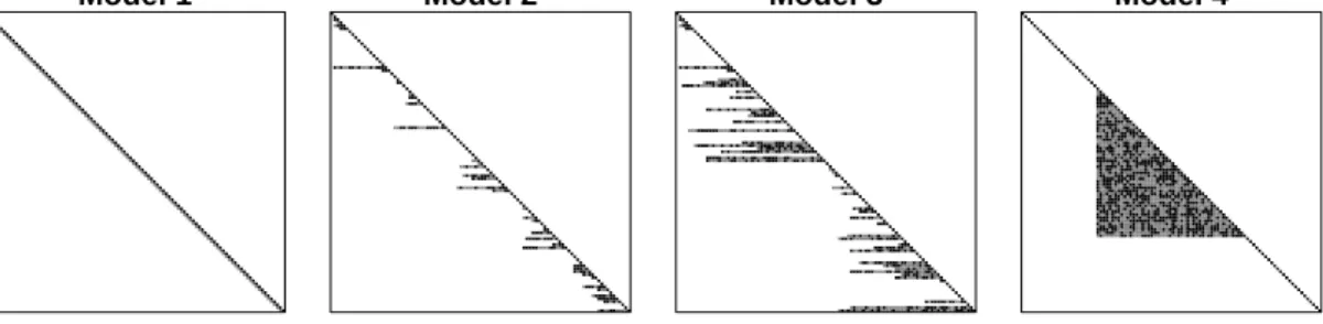
r. . . 15 2.3 Schematic of four simulation scenarios with p = 100: (from left

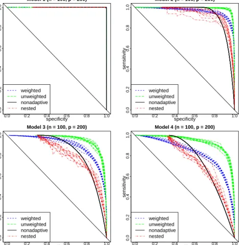
to right) Model 1 is strictly banded, Model 2 has small variable bandwidth, Model 3 has large variable bandwidth, and Model 4 is block-diagonal. Black, gray, and white stand for positive, neg-ative, and zero entries, respectively. The proportion of elements that are non-zero is 4%, 6%, 15%, and 26%, respectively. . . 30 2.4 ROC curves showing support recovery when the true L

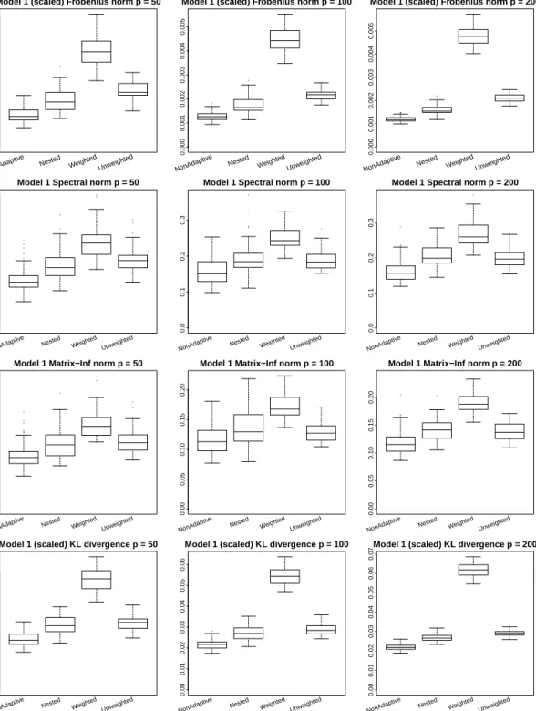
(top-left) is strictly banded, (top-right) has small variable bandwidth, (bottom-left) has large variable bandwidth, and (bottom-right) is block-diagonal, over 10 replications. . . 32 2.5 Estimation accuracy when data are generated from Model 1,

which is strictly banded. . . 35 2.6 Estimation accuracy when data are generated from Model 2,

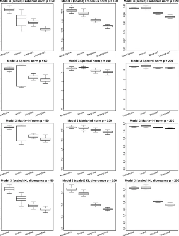
which has small variable bandwidth. . . 36 2.7 Estimation accuracy when data are generated from Model 3,

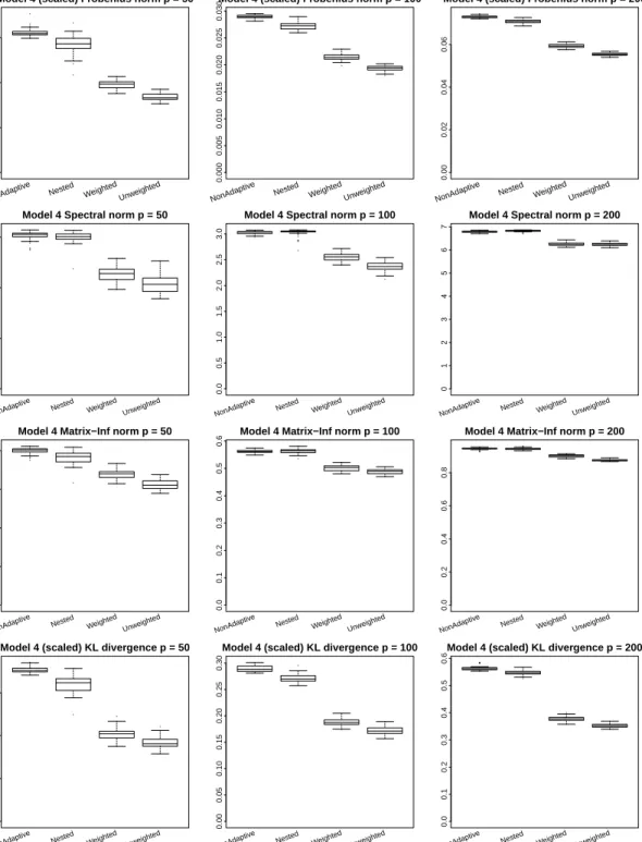
which has large variable bandwidth. . . 37 2.8 Estimation accuracy when data are generated from Model 4,

which is block-diagonal. . . 38 2.9 Prediction error (computed on an independent test set) of the

weighted (left), unweighted (middle), and CSCS (right) estimators. 41 2.10 Estimates of linkage disequilibrium with tuning parameters

se-lected by the one-standard-error rule and their corresponding precision matrix estimates. . . 42 3.1 Simulation results of methods using cross-validation. From left

to right, columns show the average (over 1000 repetitions) of the mean squared error (top panel) and E( ˆσ/σ) (bottom panel) of various methods in three simulation settings. Line styles and their corresponding methods: for naive, for σˆ2_R, for the square-root/scaled lasso, for the natural lasso, for the or-ganic lasso, for the oracle. . . 63

(12)

3.2 Simulation results of methods using pre-specified regularization parameter values. From left to right, column show the average (over 1000 repetitions) of the mean squared error (top panel) and

E( ˆσ/σ) (bottom panel) of various methods in three simulation settings. Line styles and their corresponding methods: for or-ganic (λ0), for organic (λ2), for organic (λ3), for scaled(1),

for scaled (2), for the oracle. . . 65 4.1 An example of the perfect binary tree, representing main effects.

Node value represents the success probability (rounded to 1 dec-imal place) of the corresponding Bernoulli random variable. . . . 90 4.2 Prediction mean-squared error of different methods (averaged

over 100 repetitions, binary settings). . . 92 4.3 Prediction mean-squared error of different methods (averaged

over 100 repetitions, Gaussian settings) . . . 94 4.4 Computation time and prediction mean-squared error for

differ-ent pin the mixed model. . . 95 B.1 Simulation results of various methods with regularization

pa-rameter selected using cross-validation. From left to right, col-umn show the average (over 1000 repetitions) of the mean squared error (top panel) and E( ˆσ/σ) (bottom panel) of vari-ous methods in three simulation settings. In each setting, we fix model sparsity (α) and correlations among features (ρ), and let signal-to-noise ratio(as expressed in τ) change. Line styles and their corresponding methods: for naive, for σˆ2_R, for the square-root/scaled lasso, for the natural lasso, for the organic lasso, for the oracle. . . 154 B.2 Simulation results of various methods with pre-specified

regu-larization parameter values. From left to right, column show the average (over 1000 repetitions) of the mean squared error (top panel) and E( ˆσ/σ) (bottom panel) of various methods in three simulation settings. In each setting, we fix model sparsity (α) and correlations among features (ρ), and let signal-to-noise ra-tio(as expressed in τ) change. Line styles and their correspond-ing methods: for organic (λ0), for organic (λ2), for organic (λ3), for scaled(1), for scaled (2), for the oracle. . . 155

(13)

CHAPTER 1

INTRODUCTION

With the development of new data-measurement technologies and computing power, high-dimensional data are ubiquitous in contemporary research fields, including biology, genetics, and information technologies. The notion of “high dimensionality” usually refers to the situation in which the number of predic-tors (i.e., the unknown feature parameters associated with an object) is much larger (usually in order of magnitude) than the sample size (i.e., the number of objects of interest). High-dimensionality poses a serious challenge to re-searchers who want to exploit informative patterns from large and complex data. Indeed, many traditional statistical methods no longer work in the pres-ence of high dimensionality. It is very important yet challenging to build new, accurate and stable models for properly analyzing this type of data.

Recent years have witnessed great successes and advances in statistical methodology for learning high-dimensional data, both from theoretical and computational perspectives (see, e.g., Hastie et al. 2011, B ¨uhlmann & Van De Geer 2011). A typical setting considers

Y = f(X1,X2,· · · ,Xp)+ε, (1.1) where the whole data set consists ofnindependent observation pairs of (Y,X), whereY is the response variable andX =(X1,X2,· · · ,Xp)is the predictor vector. The unobserved error (or noise)εhas mean zero and varianceσ2_{, and is} inde-pendent of X. The unknown functional f characterizes how the p predictors relate to the response variable Y, whileσ2 _{captures the noise level or extent to} whichYcannot be predicted fromX. The high-dimensional setting corresponds to the case in whichn p. There are three different components of (1.1): (1)

(14)

the random vectorX; (2) the random errorε; and (3) the function f. This thesis proposes three methods, one for modeling each of these components.

The thesis begins in Chapter 2 with a method to model local dependence structure among ppredictorsX1,· · · ,Xp. For many known f, it is helpful to first understand how theXj’s are related to each other for better prediction ofY. In many other settings whereY is not observed, it is of primary interest to study the dependence structure among theXj’s. Many applications feature a natural ordering among elements of the random vectorX. For example,(X1,· · · ,Xp)can be some variables of interest recorded over time or some genetic mutation in-formation measured along a human chromosome. Ordered variables depend on their predecessors (in the ordering). Such structure can be characterized by a simple model, which corresponds to learning the Cholesky factor of the in-verse of the covariance matrix (i.e., the precision matrix) of X. The proposed method estimates such local dependence structure by minimizing a convex pe-nalized criterion, where the penalty is designed to induce structured sparsity that honors the ordered information in the variables.

The second component in (1.1) is the error variance σ2_{, which measures} the irreducible error in modeling the dependence relationship betweenY and

X. The problem of estimatingσ2 _{is actually both important and hard in many} cases, and is underdeveloped compared with the vast literature in learning f. In Chapter 3 we propose two estimators ofσ2_{in a setting where} _f₍_X₎₌ _XT_β∗

is the standard linear model and sparsity of β∗

is assumed. The proposed estimates are remarkably simple, and they obtain statistical properties that do not depend on any assumptions onXorβ∗

.

(15)

between the responseY and the predictorsX. In numerous situations, additive models f(X)=P

jXjβ∗j (i.e., using only main effectsX) are insufficient to predict

Y. Many complex systems involve interactions among predictors, and it is im-portant to include these interactions in f to accurately model reality. Variable selection in interaction models with a large value of pis computationally very challenging because the number of interactions grows quadratically inp. Struc-tural assumptions are usually imposed to facilitate computation. In Chapter 4 we propose a computationally viable approach to interaction modeling without requiring any structural assumptions on the interactions. The proposed method scales well to large problem, enjoys theoretical guarantees on its performance, and compares favorably with alternative methods.

(16)

CHAPTER 2

LEARNING LOCAL DEPENDENCE IN ORDERED DATA

Portions of this chapter were published in Yu & Bien (2017b)

2.1

Introduction

Estimating large inverse covariance matrices is a fundamental problem in mod-ern multivariate statistics. Consider a random vector X = X1, . . . ,Xp

T

∈ _Rp with mean zero and covariance matrixE(XXT) = Σ. Unlike the covariance ma-trix, which captures marginal correlations among variables in X, the inverse covariance matrix Ω = Σ−1 _{(also known as the precision matrix) characterizes} conditional correlations and, under a Gaussian model, Ωjk = 0 implies that Xj andXkare conditionally independent given all other variables. When pis large, it is common to regularize the precision matrix estimator by making it sparse (see, e.g., Pourahmadi 2013). This paper focuses on the special context in which variables have a natural ordering, such as when data are collected over time or along a genome. In such a context, it is often reasonable to assume that random variables that are far away in the ordering are less dependent than those that are close together. For example, it is known that genetic mutations that occur close together on a chromosome are more likely to be coinherited than mutations that are located far apart. We propose a method for estimating the precision matrix based on this assumption while also allowing each random variable to have its own notion of closeness.

(17)

order-ing, two main types of convex methods with strong theoretical results have been developed for introducing sparsity in Ω. The first approach, known as the graphical lasso (Yuan & Lin 2007, Banerjee et al. 2008, Friedman et al. 2008, Rothman et al. 2008), performs penalized maximum likelihood, solving min_Ω0,Ω=ΩTL(Ω) + λP(Ω), where L(Ω) = −log detΩ + n−1Pn_i₌₁xT

i Ωxi is, up to constants, the negative log-likelihood of a sample of n independent Gaussian random vectors andP(Ω)is the (vector)`1-norm ofΩ. Zhang & Zou (2014) in-troduce a new convex loss function called theD-trace loss and propose a pos-itive definite precision matrix estimator by minimizing an `1-penalized ver-sion of this loss. The second approach is through penalized pseudo-likelihood, the most well-known of which is calledneighborhood selection (Meinshausen & B ¨uhlmann 2006). Estimators in this category are usually solved by a column-by-column approach and thus are more amenable to theoretical analysis (Yuan 2010, Cai et al. 2011, Liu & Luo 2012, Liu et al. 2017, Sun & Zhang 2013, Khare et al. 2014). However they are not guaranteed to be positive definite and do not exploit the symmetry of Ω. Peng et al. (2009) propose a partial correlation matrix estimator that develops a symmetric version of neighborhood selection; however, positive definiteness is still not guaranteed.

In the context of variables with a natural ordering, by contrast, almost no work uses convex optimization to flexibly estimate Ω while exploiting the or-dering structure. Sparsity is usually induced via the Cholesky decomposition ofΣ, which leads to a natural interpretation of sparsity. Consider the Cholesky decompositionΣ = QQT, which impliesΩ =LTLforL=Q−1for lower triangular matrices Qand Lwith positive diagonals. The assumption that X ∼ N(0,Σ)is then equivalent to a set of linear models in terms of rows of L, i.e., L11X1 = ε1

(18)

and LrrXr= − r−1 X k=1 LrkXk+εr r= 2, . . . ,p, (2.1) where ε ∼ N0,Ip

. Thus, Lrk = 0 (for k < r) can be interpreted as meaning that in predicting Xr from the previous random variables, one does not need to knowXk. This observation has motivated previous work, including Pourah-madi (1999), Wu & PourahPourah-madi (2003), Huang et al. (2006), Shojaie & Michai-lidis (2010), Khare et al. (2016). While these methods assume sparsity inL, they do not require local dependence because each variable is allowed to be depen-dent on predecessors that are distant from it (compare the upper left to the up-per right panel of Figure 2.10).

The assumption of “local dependence” can be expressed as saying that each variableXrcan be best explained by exactly itsKrclosest predecessors:

LrrXr =− r−1 X k=r−Kr LrkXk+εr, for Lrk ,0, r−Kr≤ k≤r−1, r =2, . . . ,p. (2.2) Note that this does not describe all patterns of a variable depending on its nearby variables. For example, Xr can be dependent on Xr−2 but not on Xr−1. In this case, the dependence is still local, but would not be captured by (2.2). We focus on the restricted class (2.2) since it greatly simplifies the interpretation of the learned dependence structure by capturing the extent of this dependence in a single numberKr, the neighborhood size.

Another desirable property of model (2.2) is that it admits a simple connec-tion between the sparsity pattern of Land the sparsity pattern of the precision matrixΩ in the Gaussian graphical model. In particular, straightforward

(19)

alge-bra shows that for j<k,

Lk j= · · ·= Lp j =0 =⇒ Ωjk =0. (2.3) Statistically, this says that if none of the variables Xk, . . . ,Xp depends on Xj in the sense of (2.1), thenXj and Xk are conditionally independent given all other variables.

Bickel & Levina (2008) study theoretical properties in the case that all band-widths, Kr, are equal, in which case model (2.2) is a Kr-ordered antedepen-dence model (Zimmerman & Nunez-Anton 2009). A banded estimate of L

then induces a banded estimate ofΩ. Thenested lassoapproach of Levina et al. (2008) provides for “adaptive banding”, allowingKrto vary withr (which cor-responds to variable-order antedependence models in Zimmerman & Nunez-Anton 2009); however, the nested lasso is non-convex, meaning that the pro-posed algorithm does not necessarily minimize the stated objective and theoret-ical properties of this estimator have not been established.

In this paper, we propose a penalized likelihood approach that provides the flexibility of the nested lasso but is formulated as a convex optimization prob-lem, which allows us to prove strong theoretical properties and to provide an efficient, scalable algorithm for computing the estimator. The theoretical devel-opment of our method allows us to make clear comparisons with known results for the graphical lasso (Rothman et al. 2008, Ravikumar et al. 2011) in the non-ordered case. Both methods are convex penalized likelihood approaches, so this comparison highlights the similarities and differences in the ordered and non-ordered problems.

There are two key choices we make that lead to a convex formulation. First, we express the optimization problem in terms of the Cholesky factor L. The

(20)

nested lasso and other methods (starting with Pourahmadi 1999) use the modi-fied Cholesky decomposition,Ω =TTD−1T, whereTis a lower-triangular matrix with ones on its diagonal andDis a diagonal matrix with positive entries. While

L(Ω)is convex inΩ, the negative log-likelihoodL(TT_D−1_T₎_{is not jointly convex} inT andD. By contrast, LLTL= −log detLTL+ 1 n n X i=1 xTi L T Lxi =−2 p X r=1 logLrr+ 1 n n X i=1 kLxik2₂ (2.4) is convex in L. This parametrization is considered in Aragam & Zhou (2015), Khare et al. (2014), and Khare et al. (2016). Maximum likelihood estimation ofL

preserves the regression interpretation by noting that

LLTL= −2 p X r=1 logLrr+ 1 n p X r=1 n X i=1 L2rr       xir+ r−1 X k=1 Lrkxik/Lrr        2 .

This connection has motivated previous work with the modified Cholesky de-composition, in which Trk = −Lrk/Lrr are the coefficients of a linear model in whichXris regressed on its predecessors, andDrr =L−2rr corresponds to the error variance. The second key choice is our use of a hierarchical group lasso in place of the nested lasso’s nonconvex penalty.

We introduce here some notation used throughout the paper. For two se-quences of constants a(n) and b(n), the notationa(n) = o(b(n)) means that for everyε > 0, there exists a constant N > 0such that |a(n)/b(n)| ≤ εfor all n ≥ N. And the notationa(n) = O(b(n)) means that there exists a constantN > 0and a constantM >0such that|a(n)/b(n)| ≤ Mfor alln≥ N. For a sequence of random variables A(n), the notation A(n) = OP(b(n)) means that for every ε > 0, there exists a constantM >0such thatP (|A(n)/b(n)|> M)≤ε_{for all}n.

For a vectorv = v1, . . . ,vp ∈ _Rp , we definekvk₁ = Pp j=1|vj|,kvk2 = ( Pp j=1v 2 j) 1/2 andkvk∞ = maxj|vj|. For a matrix M ∈ Rn×p, we define the element-wise norms

(21)

by two vertical bars. Specifically,kMk∞ =maxjk|Mjk|and Frobenius normkMkF = (P

j,kM2jk)

1/2_{. For}_q_≥ ₁_{, we define the matrix-induced (operator)}_q_{-norm by three} vertical bars: |||M|||q = maxkvkq=1kMvkq. Important special cases include|||M|||2, also

known as the spectral norm, which is the largest singular value of M, as well as

|||M|||₁ = maxkPp

j=1|Mjk|and |||M|||∞ = maxjP p

k=1|Mjk|. Note that|||M|||1 = |||M|||∞ when

Mis symmetric.

Given a p-vectorv, ap×pmatrixM, and an index setT, letvT = (vi)i∈T be the

|T|_{-subvector and}MT thep× |T|submatrix with columns selected fromT. Given a second index setT0, letMT T0 be the|T| × |T0|submatrix with rows and columns

ofMindexed byT andT0

, respectively. Specifically, we useLr·to denote ther-th row ofL.

2.2

Estimator

For a given tuning parameterλ≥0, we define our estimatorLˆ to be a minimizer of the following penalized negative Gaussian log-likelihood

ˆ L∈ arg min L:Lrr>0 Lrk=0forr<k        −2 p X r=1 logLrr+ 1 n n X i=1 kLxik2₂+λ p X r=2 Pr(Lr·)        . (2.5)

The penaltyPr, which is applied to ther-th row, is defined by

Pr(Lr·)= r−1 X `=1 W (`)_∗ Lgr,` ₂ = r−1 X `=1        ` X m=1 w2_`mL 2 rm        1/2 , (2.6) where W(`) = ₍_w

`1, . . . ,w``) ∈ R` is a vector of weights, ∗ denotes element-wise multiplication, and Lgr,` denotes the vector of elements of Lfrom the group gr,`,

which corresponds to the first` elements in ther-th row (for1≤` ≤r−1):

(22)

Sincegr,1 ⊂ gr,2 ⊂ · · · ⊂ gr,r−1, each row r of L is penalized with a sum of r−1 nested, weighted`2-norm penalties. This is a hierarchical group lasso penalty (Yuan & Lin 2007, Zhao et al. 2009, Jenatton et al. 2011, Yan & Bien 2015) with group structure conveyed in Figure 2.1.

With w`m > 0, this nested structure always puts more penalty on those ele-ments that are further away from the diagonal. Since the group lasso has the ef-fect of setting to zero a subset of groups, it is apparent that this choice of groups ensures that whenever the elements in gr,` are set to zero, elements in gr,`0 are

also set to zero for all`0_≤ _{`. In other words, for each row of} _ˆ

L, the non-zeros are those elements within some (row-specific) distance of the diagonal. This is in contrast to the`1-penalty as used in Khare et al. (2016), which produces sparsity patterns with no particular structure (compare the top-left and top-right panels of Figure 2.10).

The choice of weights,w`m, affects both the empirical and theoretical

perfor-mance of the estimator. We focus primarily on a quadratically decaying set of weights,

w`m=

1

(`−m+1)2, (2.7)

but also consider the unweighted case (in whichw`m = 1). The decay counter-acts the fact that the elements of L appear in differing numbers of groups (for example Lr1 appears in r −1 groups whereas Lr,r−1 appears in just one group). In a related problem, Bien et al. (2016) choose weights that decay more slowly with ` −m than (2.7). Our choice makes the enforcement of hierarchy weaker so that our penalty behaves more closely to the lasso penalty (Tibshirani 1996). The choice of weight sequence in (2.7) is more amenable to theoretical analysis; however, in practice the unweighted case is more efficiently implemented and

(23)

L11 0 0 0 0 L11 0 0 0 0 Lˆ11 0 0 0 0

L21 L22 0 0 0 L21 L22 0 0 0 0 Lˆ22 0 0 0

L31 L32 L33 0 0 L31 L32 L33 0 0 Lˆ31 Lˆ32 Lˆ33 0 0

L41 L42 L43 L44 0 L41 L42 L43 L44 0 0 0 Lˆ43 Lˆ44 0

L51 L52 L53 L54 L55 L51 L52 L53 L54 L55 0 Lˆ52 Lˆ53 Lˆ54 Lˆ55

Figure 2.1: There are₂pgroups used in the penalty, with each rowrhaving

r−1nested groupsgr,1 ⊂ gr,2 ⊂ · · · ⊂gr,r−1. Left: the groupg4,3. Middle: the nested group structureg4,1 ⊂ g4,2 ⊂ g4,3. Right: A possible sparsity pattern inLˆ, where elements in g2,1,g4,2 (and thusg4,1) andg5,1are set to zero.

works well empirically.

Problem (2.5) is convex inL. While−log det(·)is strictly convex,−P

rlog(Lrr) is not strictly convex inL. Thus, thearg minin (2.5) may not be unique. In Section 2.4, we provide sufficient conditions to ensure uniqueness with high probability.

In Appendix A.1, we show that (2.5) decouples into pindependent subprob-lems, each of which estimates one row of L. More specifically, letX ∈ _Rn×p be a sample matrix with independent rows xi ∼ N(0,Σ), Lˆ11 = n1/2(XT₁X1)−1/2 and for

r= 2, . . . ,p, ˆ Lr,1:r =arg min β∈Rr:βr>0          −2 logβr+ 1 nkX1:rβk 2 2+λ r−1 X `=1        ` X m=1 w2_`_mβ2_m        1/2         . (2.8)

This observation means that the computation can be easily parallelized, which potentially can achieve a linear speed up with the number of CPU cores. Theo-retically, to analyze the properties ofLˆ it is easier to start by studying an estima-tor of each row, i.e., a solution to (2.8). We will see in Section 2.4 that problem (2.8) has connections to a penalized regression problem, meaning that both the assumptions and results we can derive are better than if we were working with

(24)

a penalty based onΩ.

In light of the regression interpretation of (2.1), Lˆ provides an interpretable notion of local dependence; however, we can of course also use our estimate ofL to estimateΩ: Ω =ˆ _LˆT_L_ˆ_{. By construction, this estimator is both symmetric} and positive definite. Unlike a lasso penalty, which would induce unstructured sparsity in the estimate of L and thus would not be guaranteed to produce a sparse estimate ofΩ, the adaptively banded structure in our estimator ofLcan yield a generally banded Ωˆ with sparsity pattern determined by (2.3) (See the top-left and bottom-left panels in Figure 2.10 for an example).

2.3

Computation

As observed above, we can compute Lˆ by solving (in parallel across r) prob-lem (2.8). Consider an alternating direction method of multipliers (ADMM) approach that solves the equivalent problem

min β,γ∈Rr:βr>0          −2 logβr+ 1 nkX1:rβk 2 2+λ r−1 X `=1        ` X m=1 w2_`mγ 2 m        1/2 s.t. β=γ          .

Algorithm 1 presents the ADMM algorithm, which repeatedly minimizes this problem’s augmented Lagrangian over β, then over γ, and then updates the dual variableu ∈_Rr_{. The main computational effort in the algorithm is in} solv-ing (2.9) and (2.10). Note that (2.9) has a smooth objective function. Straight-forward calculus gives the closed-form solution (see Appendix A.2 for detailed derivation), β(t+1) r = −B− √ B2₋₈_A 2A > 0 β(t+1) −r =− 2S(r)−r,−r+ρI −1 2S(r)−r,rβ(tr+1)+u (t) −r−ργ (t) −r ,

(25)

Algorithm 1: ADMM algorithm to solve (2.8) Require: β(0)_,_γ(0)_,_u(0)_,_{ρ >}_0,_t₌ _1. 1: repeat 2: β(t) _←_{arg min} β∈Rr:βr>0 ( −2 logβr+ 1 nkX1:rβk 2 2+ β−γ(t−1)Tu(t−1)+ ρ 2 β−γ (t−1) 2 2 ) (2.9) 3: γ(t) _←_{arg min} γ∈Rr          ρ 2 γ−β (t)₋_ρ−1_u(t−1) 2 2+λ r−1 X `=1        ` X m=1 w2_`_mγ2_m        1/2         (2.10) 4: u(t)← u(t−1)+ρβ(t)−γ(t) 5: t← t+1 6: untilconvergence 7: returnγ(t) where S(r) = 1 nX T 1:rX1:r A=4S(r)r,−r 2S−r(r),−r+ρI −1 S(r)−r,r−2S(r)r,r−ρ <0 B=2S(r)r,−r 2S−r(r),−r+ρI −1 u(t)−r−ργ (t) −r −u(t)_r +ργ(t)_r .

The closed-form update above involves matrix inversion. With ρ > 0, the matrix 2S−r(r),−r + ρI is invertible even when r > n. Since determining a good choice for the ADMM parameterρis in general difficult, we adapt the dynamic ρupdating scheme described in Section 3.4.1 of Boyd et al. (2011).

(26)

group lasso with general weights. We adopt the strategy developed in Bien et al. (2016) (based on a result of Jenatton et al. 2011), which solves the dual problem of (2.10) by performing Newton’s method on at most r−1univariate functions. The detailed implementation is given in Algorithm 5 in Appendix A.3. Each application of Newton’s method corresponds to performing an ellip-tical projection, which is a step of blockwise coordinate ascent on the dual of (2.10) (see Appendix A.4 for details). Finally we observe in Algorithm 2 that for the unweighted case (w`m =1), solving (2.10) is remarkably efficient.

Algorithm 2: Algorithm for solving (2.10) for unweighted estimator

Require: β(t)_,_u(t−1) _∈ Rr,λ, ρ >0. 1: Initializeγ(t)₌ _β(t)₊_u(t−1)_/ρ_and_τ₌_λ/ρ 2: for`= 1, . . . ,r−1do γ(t) 1:` ←       1 − τ γ(t) 1:` ₂        + γ(t) 1:` 3: returnγ(t)_.

TheRpackagevarbandprovidesC++implementations of Algorithms 1 and 2.

2.4

Statistical properties

In this section we study the statistical properties of our estimator. In what fol-lows, we consider a lower triangular matrixLhaving row-specific bandwidths,

(27)

non-zero off-diagonals (of sizeKr) is denotedIr = {Jr+1, . . . ,r−1}. We also denote

Ic

r = {1,2, . . . ,r} \ Ir. See Figure 2.2 for a graphical example ofK5,J5,I4, andI c 4. L11 0 0 0 0 0 L22 0 0 0 L31 L32 L33 0 0 0 L42 L43 L44 0 0 0 L53 L54 L55 I4={2,3},I4c={1,4} J5= 2 K5= 2

Figure 2.2: Schematic showingJr,Kr,Ir, andIc r.

Our theoretical analysis is built on the following assumptions:

A1 Gaussian assumption: The sample matrixX ∈_Rn×p hasnindependent rows

with each rowxidrawn from N(0,Σ).

A2 Sparsity assumption: The true Cholesky factorL∈_Rp×pis the lower

triangu-lar matrix with positive diagonal elements such that the precision matrix

Ω = Σ−1 ₌ _LT

L. The matrix L has row-specific bandwidths Kr such that

Lr j =0for0< j<r−Kr.

A3 Irrepresentable condition: There exists someα∈(0,1]such that

max 2≤r≤pmax`∈Ic r Σ`Ir ΣIrIr −1 ₁≤ 6 π2 (1−α)

A4 Bounded singular values: There exists a constantκsuch that

(28)

When maxrKr < n, the Gaussianity assumptionA1 implies thatXIr has full

column rank for allr with probability one. Our analysis applies to the general high-dimensional scaling scheme whereKr = Kr(n)and p= p(n)can grow with

n. Forr =2, . . . ,pand` ∈ Ic r = {1, . . . ,Jr,r}, let θ(`) r := Var X`|XIr and θr :=max `∈Ic r θ(`) r . By Assumption A1, θ(r`) = Σ`` − Σ`Ir ΣIrIr −1Σ

Ir` represents the noise variance

when regressingX`on XIr, i.e., for`= 1, . . . ,Jr,r,

X` = Σ`Ir(ΣIrIr) −1_XT Ir +E` with E` ∼ N 0, θ(`) r . (2.11)

In words,θ(r`)measures the degree to whichX`cannot be explained by the vari-ables in the support andθris the maximum such value over all`outside of the supportIr in ther-th row. Intuitively, the difficulty of the estimation problem increases withθr. Note that forr= 1, . . . ,p, (2.1) impliesθ(r)r =1/L2rr.

AssumptionA3(along with theβmincondition) is essentially a necessary and sufficient condition for support recovery of lasso-type methods (see, e.g., Zhao & Yu 2006, Meinshausen & B ¨uhlmann 2006, Wainwright 2009, Van de Geer & B ¨uhlmann 2009, Ravikumar et al. 2011). The constant α ∈ (0,1] is usually re-ferred to as the irrepresentable (incoherence) constant (Wainwright 2009). In-tuitively, the irrepresentable condition requires low correlations between signal and noise predictors, and thus a value ofαthat is close to 1 implies that recov-ering the support is easier to achieve. The constant 6π−2 _{is determined by the} choice of weight (2.7) and can be eliminated by absorbing its reciprocal into the definition of the weightsw`m. Doing so, one finds that our irrepresentable

con-dition is essentially the same as the one found in the regression setting (Wain-wright 2009) despite the fact that our goal is estimating a precision matrix.

(29)

Assumption A4is a bounded singular value condition. Recalling that Ω =

LTL,

0< κ−2 ≤σ_min(Σ)≤σ_max(Σ)≤ κ2, _(2.12)

which is equivalent to the commonly used bounded eigenvalue condition in other literatures.

2.4.1

Row-specific results

We start by analyzing support recovery properties of our estimator for each row, i.e., the solution to the subproblem (2.8). Forr > n, the Hessian of the negative log-likelihood is not positive definite, meaning that the objective function may not be strictly convex inβand the solution not necessarily unique. Intuitively, if the tuning parameterλis large, the resulting row estimateLˆr·is sparse and thus includes most variation in a small subset of thervariables. More specifically, for largeλ, Iˆr ⊆ Ir and thus by AssumptionA1, XIˆr has full rank, which implies

that Lˆr· is unique. The series of technical lemmas in Appendix A.5 precisely characterizes the solution.

The first part of the theorem below shows that with an appropriately chosen tuning parameterλthe solution to (2.8) is sparse enough to be unique and that we will not over-estimate the true bandwidth. Knowing that the support of the unique row estimatorLˆr·is contained in the true support reduces the dimension of the parameter space, and thus leads to a reasonable error bound. Of course, if our goal were simply to establish the uniqueness of Lˆr· and thatKˆr ≤ Kr, we could trivially takeλ = ∞ _{(resulting in} Kˆr = 0). The latter part of the theorem thus goes on to provide a choice ofλthat is sufficiently small to guarantee that

(30)

ˆ

Kr = Kr (and, furthermore, that the signs of all non-zeros are correctly recov-ered).

Theorem 1. Consider the family of tuning parameters

λ= _α8

r

θrlogr

n (2.13)

and weights given by(2.7). Under AssumptionsA1–A4, if the tuple(n,Jr,Kr)satisfies

n> α−23π2Kr+8

θrκ2_log_J_r,

(2.14)

then with probability greater than1−c1exp−c2min(Kr,logJr) −7 exp (−c3n)for some

constantsc1,c2,c3independent ofnandJr, the following properties hold:

1. The row problem(2.8)has a unique solutionLˆr· andKˆr ≤ Kr.

2. The estimate Lˆr·satisfies the element-wise`∞bound,

Lˆr·−Lr· _∞ ≤ λ 4 ΣIrIr −1 _∞+5κ 2 . (2.15) 3. If in addition, min j≥Jr+1 Lr j > λ 4 ΣIrIr −1 _∞+5κ 2_, _(2.16)

then exact signed support recovery holds: For all j≤r,sign( ˆLr j)=sign(Lr j).

Proof. See Appendix A.6.

In the classical setting where the ambient dimensionris fixed and the sample size n is allowed to go to infinity,λ → 0and the above scaling requirement is satisfied. By (2.15) the row estimatorLˆr·is consistent as is the classical maximum likelihood estimator. Moreover, it recovers the true support since (2.16) holds automatically. In high-dimensional scaling, however, bothnandr are allowed

(31)

to change, and we are interested in the case wherercan grow much faster thann. Theorem 1 shows that, if

ΣIrIr −1

_∞ = O(1)and ifncan grow as fast asKrlogJr,

then the row estimatorLˆr· still recovers the exact support ofLr·when the signal is at least O(

q

logr

n ) in size, and the estimation error maxj|Lˆr j − Lr j|is O(

q

logr n ). Intuitively, for the row estimator to detect the true support, we require that the true signal be sufficiently large. The condition (2.16) imposes limitations on how fast the signal is allowed to decay, which is the analogue to the commonly known “βmincondition” that is assumed for establishing support recovery of the lasso.

Remark 2. Both the choice of tuning parameter(2.13)and the error bound (2.15) de-pend on the true covariance matrix via θr. This quantity can be bounded by κ2 _{as in} (2.12)using the fact that ΣIrIr

−1 is positive definite: θr =max `∈Ic r θ(`) r =max `∈Ic r n Σ``−Σ`Ir ΣIrIr −1Σ Ir` o ≤max `∈Ic r Σ`` ≤ κ2.

The proof of Theorem 1 shows that the results in this theorem still hold true if we replace

θrbyκ2_{. This observation leads to the fact that we can select a tuning parameter having}

the properties of the theorem that does not depend on the unknown sparsity level Kr.

Therefore, our estimator is adaptive to the underlying unknown bandwidths.

Connections to the regression setting

In (2.1) we showed that estimation of the r-th row of L can be interpreted as a regression of Xr on its predecessors. It is thus very interesting to compare Theorem 1 to the standard high-dimensional regression results. Consider the following linear model of a vectory∈_Rn

of the form

(32)

where η ∈ _Rp

is the unknown but fixed parameter to estimate, Z ∈ _Rn×p is the design matrix with each row an observation ofppredictors,σ2_{is the variance of} the zero-mean additive noiseω. A standard approach in the high-dimensional setting where p n is the lasso (Tibshirani 1996), which solves the convex optimization problem, min η∈Rp 1 2nky−Zηk 2 2+λkηk1, (2.18)

where λ > 0 is a regularization parameter. In the setting where η is assumed to be sparse, the lasso solution is known to be able to successfully recover the signed support of the trueηwith high probability whenλis of the scaleσ

q

logp n and certain technical conditions are satisfied (Wainwright 2009).

Despite the added complications of working with thelogterm in the objec-tive of (2.8), Theorem 1 gives a clear indication that, in terms of difficulty of sup-port recovery, the row estimate problem (2.8) is essentially the same as a lasso problem with random design, i.e., with each rowzi ∼ N(0,Σ)(Theorem 3, Wain-wright 2009). Indeed, a comparison shows that the two irrepresentable condi-tions are equivalent. Moreover, θr plays the same role as Wainwright (2009)’s maxiΣSc_Sc−Σ_Sc_S (Σ_{S S})−1Σ_{S S}c

ii, a threshold constant of the conditional covari-ance, whereS is the support of the trueη.

St¨adler et al. (2010) introduce an alternative approach to the lasso, in the context of penalized mixture regression models, that solves the optimization problem, ( ˆφ,ρ)ˆ = arg min φ,ρ ( −2 logρ+ 1 nkρy+Zφk 2 2+λkφk1 ) , (2.19)

where σˆ = ρˆ−1 _and η_ˆ = ₋φ/_ˆ ρ_ˆ_{. Note that (2.19) basically coincides with (2.8)} except for the penalty.

(33)

In St¨adler et al. (2010), the authors study the asymptotic and non-asymptotic properties of the`1-penalized estimator for the general mixture regression mod-els where the loss functions are non-convex. The theoretical properties of (2.19) are studied in Sun & Zhang (2010), which partly motivates the scaled lasso (Sun & Zhang 2012).

The theoretical work of Sun & Zhang (2010) differs from ours both in that they study the `1 penalty (instead of the hierarchical group lasso) and in their assumptions. The nature of our problem requires the sample matrix to be ran-dom (as in A1), while Sun & Zhang (2010) considers the fixed design setting, which does not apply in our context. Moreover, they provide prediction consis-tency and a deviation bound of the regression parameters estimation in`1norm. We give exact signed support recovery results for the regression parameters as well as estimation deviation bounds in various norm criteria. Also, they take an asymptotic point of view while we give finite sample results.

2.4.2

Matrix bandwidth recovery result

With the properties of the row estimators in place, we are ready to state results about estimation of the matrix L. The following theorem gives an analogue to Theorem 1 in the matrix setting. Under similar conditions, with one particular choice of tuning parameter, the estimator recovers the true bandwidth for all rows adaptively with high probability.

Theorem 3. Letθ= maxrθrandK = maxrKr, and take λ= _α8

r

2θlogp

(34)

and weights given by(2.7). Under AssumptionsA1–A4, if(n,p,K)satisfies

n> α−2θκ212π2K+32logp, (2.21)

then with probability greater than1−cp−1_{for some constant}_c_{independent of}_n_and _p,

the following properties hold:

1. The estimator Lˆ is unique, and it is at least as sparse asL, i.e.,Kˆr≤ Krfor allr.

2. The estimator _Lˆ _{satisfies the element-wise}_`∞_bound,

Lˆ−L _∞ ≤λ 4 max r ΣIrIr −1 _∞+5κ 2_. _(2.22) 3. If in addition, min r j≥Jminr+1 Lr j > λ 4 max r ΣIrIr −1 _∞+5κ 2_, _(2.23)

then exact signed support recovery holds:sign( ˆLr j)= sign(Lr j)for allrand j.

As discussed in Remark 2, we can replace θ with its upper bound κ2_{, and} the results remain true. This theorem shows that one can properly estimate the sparsity pattern across all rows exactly using only one tuning parameter chosen without any prior knowledge of the true bandwidths. In Section 2.4.1, we noted that the conditions required for support recovery and the element-wise`∞error bound for estimating a row ofLis similar to those of the lasso in the regression setting. A union bound argument allows us to translate this into exact band-width recovery in the matrix setting and to derive a reasonable convergence rate under conditions as mild as that of a lasso problem with random design.

(35)

This technique is similar in spirit to neighborhood selection (Meinshausen & B ¨uhlmann 2006), though our approach is likelihood-based.

Comparing (2.21) to (2.14), we see that the sample size requirement for re-covering Lis determined by the least sparse row. While intuitively one would expect the matrix problem to be harder than any single row problem, we see that in fact the two problems are basically of the same difficulty (up to a multi-plicative constant).

In the setting where variables exhibit a natural ordering, Shojaie & Michai-lidis (2010) proposed a penalized likelihood framework like ours to estimate the structure of directed acyclic graphs (DAGs). Their method focuses on vari-ables which are standardized to have unit variance. In this special case, penal-ized likelihood does not involve the log-determinant term and under similar assumptions to ours, they proved support recovery consistency. However, they use lasso and adaptive lasso (Zou 2006) penalties, which do not have the built-in notion of local dependence. Since these`1-type penalties do not induce struc-tured sparsity in the Cholesky factor, the resulting precision matrix estimate is not necessarily sparse. By contrast, our method does not assume unit variances and learns an adaptively banded structure for_Lˆ _{that leads to a sparse}_Ωˆ _(thereby encoding conditional dependencies).

To study the difference between the ordered and non-ordered problems, we compare our method with Ravikumar et al. (2011), who studied the graphical lasso estimator in a general setting where variables are not necessarily ordered. Let S _{index the edges of the graph specified by the sparsity pattern of} Ω =

(36)

irrepresentable condition imposed onΓ = Σ⊗Σ ∈_Rp2_×p2 : max e∈Sc ΓeS(ΓSS) −1 ₁ ≤ (1−α) (2.24)

for some α ∈ (0,1]. Our Assumption A3 is on each variable through the en-tries of the true covarianceΣwhile (2.24) imposes such a condition on the edge variables Y(j,k) = XjXk −E

XjXk

, resulting in a vector `1-norm restriction on a much larger matrix Γ, which can be more restrictive for large p. More specif-ically, condition (2.24) arises in Ravikumar et al. (2011) to tackle the analysis of thelog detΩ term in the graphical lasso problem. By contrast, in our setting the parameterization in terms of Lmeans that thelog det term is simply a sum of log terms on diagonal elements and is thus easier to deal with, leading to the milder irrepresentable assumption. Another difference is that they require the sample size n > cκ_Γ2d2logp for some constant c. The quantity d measures the maximum number of non-zero elements in each row of the true Σ, which in our case is 2K + 1, and κΓ =

(ΓSS) −1

_∞ can be much larger thanκ

2_{. Thus,} comparing to (2.21), one finds that their sample size requirement is much more restrictive. A similar comparison could also be made with the lasso penalized D-trace estimator (Zhang & Zou 2014), whose irrepresentable condition involves

Γ =(Σ⊗I+I⊗Σ)/2∈_Rp2×p2. Of course, the results in both Ravikumar et al. (2011) and Zhang & Zou (2014) apply to estimators invariant to permutation of vari-ables; additionally, the random vector only needs to satisfy an exponential-type tail condition.

2.4.3

Precision matrix estimation consistency

Although our primary target of interest is L, the parameterization Ω = LT_L makes it natural for us to try to connect our results of estimating L with the

(37)

vast literature in directly estimatingΩ, which is the standard estimation target when the known ordering is not available. In this section, we consider the es-timation consistency of Ω using the results we obtained for L. The following theorem gives results of how wellΩ =ˆ LˆT_L_ˆ

performs in estimating the true pre-cision matrixΩ =LT_L_{in terms of various matrix norm criteria.}

Theorem 4. Letθ = maxrθr, K = maxrKr and s = PrKr denote the total number of

non-zero off-diagonal elements inL. DefineζΣ = 8

√ 2θ α 4 maxr ΣIrIr −1 _∞+5κ 2_.

Un-der the assumptions in Theorem 3, the following deviation bounds hold with probability greater than1−cp−1 for some constantcindependent ofnand p:

Ωˆ −Ω _∞ ≤2ζΣ|||L|||∞ r logp n +ζ 2 Σ(K+1) logp n , Ωˆ −Ω _∞ ≤2ζΣ|||L|||∞(K+1) r logp n +ζ 2 Σ(K+1)2 logp n , Ωˆ −Ω ₂ ≤2ζΣ|||L|||∞(K+1) r logp n +ζ 2 Σ(K+1)2 logp n , Ωˆ −Ω _F ≤2κζΣ r (s+ p) logp n +ζ 2 Σ(K+1) √ s+plogp n .

When the quantities ζ_Γ, |||L|||∞, and κ are treated as constants, these bounds can be summarized more succinctly as follows:

Corollary 5. Using the notation and conditions in Theorem 4, ifζ_Γ,|||L|||∞, andκremain

(38)

estimation error bounds: Ωˆ −Ω _∞ = OP        r logp n       , Ωˆ −Ω _∞ = OP       (K+1) r logp n       , Ωˆ −Ω ₂= OP       (K+1) r logp n       , Ωˆ −Ω _F = OP        r (s+ p) logp n       .

The conditions for these deviation bounds to hold are those required for sup-port recovery as in Theorem 3. In many cases where estimation consistency is more of interest than support recovery, we can still deliver the desired error rate in Frobenius norm, matching the rate derived in Rothman et al. (2008). In par-ticular, we can drop the strong irrepresentable assumption (A3) and weaken the Gaussian assumption (A1) to the following marginal sub-Gaussian assumption:

A5 Marginal sub-Gaussian assumption: The sample matrixX ∈_Rn×p

hasn inde-pendent rows with each row drawn from the distribution of a zero-mean random vector X = (X1,· · · ,Xp)T with covariance Σ and sub-Gaussian marginals, i.e.,

E exptXj/pΣj j

≤expCt2

for all j=1, . . . ,p,t≥ 0and for some constantC > 0that does not depend on j.

Theorem 6. Under Assumption A2, A4 and A5, with tuning parameter λ of scale

q

logp

(39)

fol-lowing estimation error bounds in Frobenius norm to hold: Lˆ −L _F =OP        r (s+p) logp n       , Ωˆ −Ω _F =OP        r (s+p) logp n       .

The rates in Corollary 5 (and Theorem 6) essentially match the rates obtained in methods that directly estimateΩ(e.g., the graphical lasso estimator, studied in Rothman et al. 2008, Ravikumar et al. 2011, and the column-by-column meth-ods as in Cai et al. 2011, Liu et al. 2017, and Sun & Zhang 2013). However, the exact comparison in rates with these methods is not straightforward. First, the targets of interest are different. In the setting where the variables have a known ordering, we are more interested in the structural information among variables that is expressed in L, and thus accurate estimation ofL is more im-portant. When such ordering is not available as considered in Rothman et al. (2008), Cai et al. (2011), Liu et al. (2017) and so on, however, the conditional de-pendence structure encoded by the sparsity pattern inΩis more of interest, and the accuracy of directly estimatingΩis the focus. Moreover, deviation bounds of different methods are built upon assumptions that treat different quantities as constants. Quantities that are assumed to remain constant in the analysis of one method might actually be allowed to scale with ambient dimension in a non-trivial manner in another method, which makes direct rate comparison among different methods complicated and less illuminating.

Our analysis can be extended to the unweighted version of our estimator, i.e., with weightw`m =1, but under more restrictive conditions and with slower rates of convergence. Specifically, AssumptionA3becomesmax`∈Ic

r Σ`Ir ΣIrIr −1 ₁ ≤

(40)

(1−α)/Kr for each r = 2, . . . ,p. With the same tuning parameter choice (2.13) and (2.20), the terms ofKr and K in sample size requirements (2.14) and (2.21) are replaced with K2

r and K2, respectively. The estimation error bounds in all norms are multiplied by an extra factor ofK. All of the above indicates that in highly sparse situations (in which K is very small), the unweighted estimator has very similar theoretical performance to the weighted estimator.

2.5

Simulation study

In this section we study the empirical performance of our estimators (both with weights as in (2.7) and with no weights, i.e., w`m = 1) on simulated data. For comparison, we include two other sparse precision matrix estimators designed for the ordered-variable case:

• Non-Adaptive Banding (Bickel & Levina 2008): This method estimates

Las a lower-triangular matrix with a fixed bandwidth K applying across all rows. The regularization parameter used in this method is the fixed bandwidthK.

• Nested Lasso(Levina et al. 2008): This method yields an adaptive banded structure by solving a set of penalized least-squares problems (both the loss function and the nested-lasso penalty are non-convex). The regular-ization parameter controls the amount of penalty and thus the sparsity level of the resulting estimate.

All simulations are run at a sample size of n = 100, where each sample is drawn independently from thep-dimensional normal distributionN(0,(LTL)−1).

(41)

We compare the performance of our estimators with the methods above both in terms of support recovery (in Section 2.5.1) and in terms of how wellLˆestimates

L(in Section 2.5.2). For support recovery, we considerp=200and for estimation accuracy, we consider p = 50,100,200, which corresponds to settings where

p<n, p=n, and p> n, respectively.

We simulate under the following models forL. We adapt the parameteriza-tionL= D−1T as in Khare et al. (2016), whereDis a diagonal matrix with diago-nal elements drawn randomly from a uniform distribution on the interval[2,5], and T is a lower-triangular matrix with ones on its diagonal and off-diagonal elements defined as follows:

• Model 1: Model 1 is at one extreme of bandedness of the Cholesky factor

L, in which we take the lower triangular matrixL ∈_Rp×p _{to have a strictly} banded structure, with each row having the same bandwidth Kr = K = 1 for allr. Specifically, we takeTr,r =1,Tr,r−1= 0.8andTr,j = 0for j< r−1. • Model 2: Model 2 is at the other extreme, in which we allow Kr to vary

withr. We takeT to be a block diagonal matrix with 5 blocks, each of size

p/5. Within each block, with probability 0.5 each rowris assigned with a non-zero bandwidth that is randomly drawn from a uniform distribution on {1, . . . ,r−1} _(for r > 1). Each non-zero element in T is then drawn independently from a uniform distribution on the interval[0.1,0.4], and is assigned with a positive/negative sign with probability 0.5.

• Model 3: Model 3 is a denser and thus more challenging version of Model 2, withT a block diagonal matrix with only 2 blocks. Each of the blocks is of sizep/2but is otherwise generated as in Model 2.

(42)

Model 1 Model 2 Model 3 Model 4

Figure 2.3: Schematic of four simulation scenarios with p=100: (from left to right) Model 1 is strictly banded, Model 2 has small variable bandwidth, Model 3 has large variable bandwidth, and Model 4 is block-diagonal. Black, gray, and white stand for positive, negative, and zero entries, respectively. The proportion of ele-ments that are non-zero is 4%, 6%, 15%, and 26%, respectively.

completely dense lower-triangular block from the p/4-th row to the3p

/4-th row and is zero everywhere else. Wi/4-thin /4-this block, all off-diagonal elements are drawn uniformly from[0.1,0.2], and positive/negative signs are then assigned with probability 0.5.

Model 1 is a stationary autoregressive model of order 1. By the regression interpretation (2.1), for each r, it can be verified that the autoregressive poly-nomial of ther-th row of Models 2, 3, and 4 has all roots outside the unit cir-cle, which characterizes stationary autoregressive models of orders equal to the corresponding row-wise bandwidths. See Figure 2.3 for examples of the four sparsity patterns forp=100. The non-adaptive banding method should benefit from Model 1 while the nested lasso and our estimators are expected to perform better in the other three models where each row has its own bandwidth.

For all four models and every value of p considered, we verified that As-sumptionsA3andA4hold and then simulatedn = 100observations according to each of the four models based on AssumptionA1.

(43)

2.5.1

Support recovery

We first study how well the different estimators identify zeros in the four models above. We generate n = 100 random samples from each model with p = 200. The tuning parameterλ≥ 0in (2.5) measures the amount of regularization and determines the sparsity level of the estimator. We use 100 tuning parameter values for each estimator and repeat the simulation 10 times.

Figure 2.4 shows the sensitivity (fraction of true non-zeros that are correctly recovered) and specificity (fraction of true zeros that are correctly set to zero) of each method parameterized by its tuning parameter (in the case of non-adaptive banding, the parameter is the bandwidth itself, ranging from0top−1). Each set of 10 curves of the same color corresponds to the results of one estimator, and each curve within the set corresponds to the result of one draw from 10 sim-ulations. Curves closer to the upper-right corner indicate better classification performance (the x+y=1line corresponds to random guessing).

The sparsity level of the non-adaptive banding estimator depends only on the pre-specified bandwidth (which is the method’s tuning parameter) and not on the data itself. Consequently, the sensitivity-specificity curves for the non-adaptive banding do not vary across replications when simulating from a partic-ular underlying model. The sparsity levels of the nested lasso and our methods, by contrast, hinge on the data, thus giving a different curve for each replication.

(44)

0.0 0.2 0.4 0.6 0.8 1.0 0.0 0.2 0.4 0.6 0.8 1.0 Model 1 (n = 100, p = 200) specificity sensitivity weighted unweighted nonadaptive nested 0.0 0.2 0.4 0.6 0.8 1.0 0.0 0.2 0.4 0.6 0.8 1.0 Model 2 (n = 100, p = 200) specificity sensitivity weighted unweighted nonadaptive nested 0.0 0.2 0.4 0.6 0.8 1.0 0.0 0.2 0.4 0.6 0.8 1.0 Model 3 (n = 100, p = 200) specificity sensitivity weighted unweighted nonadaptive nested 0.0 0.2 0.4 0.6 0.8 1.0 0.0 0.2 0.4 0.6 0.8 1.0 Model 4 (n = 100, p = 200) specificity sensitivity weighted unweighted nonadaptive nested

Figure 2.4: ROC curves showing support recovery when the true L

(top-left) is strictly banded, (top-right) has small variable bandwidth, (bottom-left) has large variable bandwidth, and (bottom-right) is block-diagonal, over 10 replications.

In practice, we find that our methods and the nested lasso sometimes pro-duce entries with very small, but non-zero, absolute values. To study support recovery, we set all estimates whose absolute values are below 10−10 _{to zero,} both in our estimators and the nested lasso.

In Model 1, we observe that all methods considered attain perfect classifica-tion accuracy for some value of their tuning parameter. While the non-adaptive approach is guaranteed to do so in this scenario, it is reassuring to see that the

(45)

more flexible methods can still perfectly recover this sparsity pattern.

In Model 2, we observe that our two methods outperform the nested lasso, which itself, as expected, outperforms the non-adaptive banding method. As the model becomes more challenging (from Model 2 to Model 4), the perfor-mances of all four methods start deteriorating. Interestingly, the nested lasso no longer retains its advantage over non-adaptive banding in Models 3 and 4, while the performance advantage of our methods become even more substan-tial.

The fact that the unweighted version of our method outperforms the weighted version stems from the fact that all models are comparatively sparse forp= 200, and so the heavier penalty on each row delivered by the unweighted approach recovers the support more easily than the weighted version.

2.5.2

Estimation accuracy

We proceed by comparing the estimators in terms of how farLˆ is fromL. To this end, we generaten = 100 random samples from the four models with p = 50,

p = 100, and p = 200. Each method is computed with its tuning parameter selected to maximize the Gaussian likelihood on the validation data in a 5-fold cross-validation. For comparison, we report the estimation accuracy of each estimate in terms of the scaled Frobenius norm 1

p Lˆ −L 2

F, the matrix infinity norm Lˆ −L

_∞, the spectral norm Lˆ−L

₂, and the (scaled) Kullback-Leibler

loss 1 p

h

tr(Ω−1_Ω_ˆ₎₋_{log det(}_Ω−1_Ω_ˆ₎₋ _pi_{(Levina et al. 2008).}

(46)

Fig-ure 2.5 through FigFig-ure 2.8. Each figFig-ure corresponds to a model, and consists of a 4-by-3 panel layout. Each row corresponds to an error measure, and each column corresponds to a value of p.

As expected, the non-adaptive banding estimator does better than the other estimators in Model 1. In Models 2, 3, and 4, where bandwidths vary with row, our estimators and the nested lasso outperform non-adaptive banding.

A similar pattern is observed as in support recovery. As the model becomes more complex and pgets larger, the performance of the nested lasso degrades and gradually becomes worse than non-adaptive banding. By contrast, as the estimation problem becomes more difficult, the advantage in performance of our methods becomes more obvious.

We again observe that the unweighted estimator performs better than the weighted one. As shown in Section 2.4, the overall performance of our method hinges on the underlying model complexity (measured in terms of maxrKr) as well as the relative size ofnand p. Whennis relatively small, usually a more constrained method (like the unweighted estimator) is preferred over a more flexible method (like the weighted estimator). So in our simulation setting, it is reasonable to observe that the unweighted method works better. Note that as the underlying L becomes denser (from Model 1 to Model 4), the perfor-mance difference between the weighted and the unweighted estimator dimin-ishes. This corroborates our discussion in the end of Section 2.4 that the perfor-mance of the unweighted estimator becomes worse when the underlying model is dense.

(47)

●

Model 1 (scaled) Frobenius norm p = 50

0.000 0.001 0.002 0.003 0.004 0.005 NonAdaptiv e

Nested _{Weighted Unw}eighted

● ●

Model 1 (scaled) Frobenius norm p = 100

0.000 0.001 0.002 0.003 0.004 0.005 NonAdaptiv e

●●● ●

Model 1 (scaled) Frobenius norm p = 200

0.000 0.001 0.002 0.003 0.004 0.005 NonAdaptiv e

● ● ● ● ● ● ● ● ● ● ● ● Model 1 Spectral norm p = 50

0.00 0.05 0.10 0.15 0.20 0.25 0.30 0.35 NonAdaptiv e

●

● ● ●

● Model 1 Spectral norm p = 100

0.0 0.1 0.2 0.3 NonAdaptiv e

● ●

●

● Model 1 Spectral norm p = 200

0.0 0.1 0.2 0.3 NonAdaptiv e

● ● ● ● ● ● ● ● ● ● ● Model 1 Matrix−Inf norm p = 50

0.00 0.05 0.10 0.15 0.20 0.25 NonAdaptiv e

Model 1 Matrix−Inf norm p = 100

0.00 0.05 0.10 0.15 0.20 NonAdaptiv e

● ●

●

Model 1 Matrix−Inf norm p = 200

0.00 0.05 0.10 0.15 0.20 NonAdaptiv e

Nested _{Weighted Unw}eighted Model 1 (scaled) KL divergence p = 50

0.00 0.01 0.02 0.03 0.04 0.05 NonAdaptiv e

●

Model 1 (scaled) KL divergence p = 100

0.00 0.01 0.02 0.03 0.04 0.05 0.06 NonAdaptiv e

● Model 1 (scaled) KL divergence p = 200

0.00 0.01 0.02 0.03 0.04 0.05 0.06 0.07 NonAdaptiv e

Figure 2.5: Estimation accuracy when data are generated from Model 1, which is strictly banded.

(48)

Model 2 (scaled) Frobenius norm p = 50 0.000 0.002 0.004 0.006 NonAdaptiv e

● ● ● ● ● ● ● ●● Model 2 (scaled) Frobenius norm p = 100

0.000 0.004 0.008 0.012 NonAdaptiv e

●●

Model 2 (scaled) Frobenius norm p = 200

0.000 0.010 0.020 0.030 NonAdaptiv e

● ●

Model 2 Spectral norm p = 50

0.0 0.2 0.4 0.6 0.8 NonAdaptiv e

● ● Model 2 Spectral norm p = 100

0.0 0.5 1.0 1.5 NonAdaptiv e

● ● ● ● ●● ● ● ●●

Model 2 Spectral norm p = 200

0 1 2 3 4 NonAdaptiv e

● ● ●● ● ● ●

0.00 0.05 0.10 0.15 0.20 0.25 0.30 NonAdaptiv e

● ● ●● ●● ●● ● ●● ●

Model 2 Matrix−Inf norm p = 100

0.0 0.1 0.2 0.3 0.4 NonAdaptiv e

● ●● ● ● ●● ● ●● ● ● ●

0.0 0.2 0.4 0.6 NonAdaptiv e

0.00 0.02 0.04 0.06 NonAdaptiv e

● ● ● ● ●● ● Model 2 (scaled) KL divergence p = 100

0.00 0.02 0.04 0.06 0.08 0.10 0.12 NonAdaptiv e

0.00 0.05 0.10 0.15 0.20 0.25 NonAdaptiv e

Figure 2.6: Estimation accuracy when data are generated from Model 2, which has small variable bandwidth.

(49)

Model 3 (scaled) Frobenius norm p = 50 0.000 0.005 0.010 0.015 0.020 0.025 NonAdaptiv e

●●●

● <

High-Dimensional Structured Regression Using Convex Optimization

HIGH-DIMENSIONAL STRUCTURED

HIGH-DIMENSIONAL STRUCTURED REGRESSION USING CONVEX OPTIMIZATION

BIOGRAPHICAL SKETCH

TABLE OF CONTENTS

4 Reluctant interaction modeling 68

LIST OF TABLES

CHAPTER 1

INTRODUCTION

CHAPTER 2

LEARNING LOCAL DEPENDENCE IN ORDERED DATA

Estimator

Computation

Statistical properties

Row-specific results

Connections to the regression setting

Matrix bandwidth recovery result

Precision matrix estimation consistency

Simulation study

Model 1 Model 2 Model 3 Model 4

Support recovery

Estimation accuracy

Model 1 (scaled) Frobenius norm p = 50

Model 1 Matrix−Inf norm p = 100

Model 2 (scaled) Frobenius norm p = 200

Model 2 Matrix−Inf norm p = 100