Voicing classification of visual speech using convolutional neural networks

Voicing classification of visual speech using convolutional neural networks

Thomas Le Cornu, Ben Milner

University of East Anglia

Abstract

The application of neural network and convolutional neural net-work (CNN) architectures is explored for the tasks of voicing classification (classifying frames as being either non-speech, unvoiced, or voiced) and voice activity detection (VAD) of vi-sual speech. Experiments are conducted for both speaker de-pendent and speaker indede-pendent scenarios.

A Gaussian mixture model (GMM) baseline system is de-veloped using standard image-based two-dimensional discrete cosine transform (2D-DCT) visual speech features, achieving speaker dependent accuracies of79% and 94%, for voicing classification and VAD respectively. Additionally, a single-layer neural network system trained using the same visual fea-tures achieves accuracies of86% and97%. A novel technique using convolutional neural networks for visual speech feature extraction and classification is presented. The voicing classifi-cation and VAD results using the system are further improved to88% and98% respectively.

The speaker independent results show the neural network system to outperform both the GMM and CNN systems, achiev-ing accuracies of63% for voicing classification, and79% for voice activity detection.

Index Terms: convolutional neural networks, voicing classifi-cation, visual speech

1. Introduction

The aim of this work is to explore using neural networks and convolutional neural networks for voicing classification and voice activity detection using visual speech features. Voicing classification is the challenge of classifying frames of speech (either audio, visual, or audiovisual) as being either non-speech, unvoiced, or voiced. The task of voice activity detection can be considered a more generalised version of the voicing classifi-cation task, classifying frames as speech or non-speech. By grouping the unvoiced and voiced classes together, the estima-tion of speech and non-speech results. The aim is to learn a function,f, to estimate the voicing class,cˆt, of the input visual

speech feature vector,vt, described by,

ˆ

ct=f(vt), (1)

whereˆcVCt ∈ {ns, u, v}for voicing classification, andˆcVADt ∈

{ns, s}for voice activity detection.

Voice activity detection systems traditionally take audio speech as input. Problems occur as the signal-to-noise ratio is lowered due to increased background noise, with VAD accura-cies decreasing as more non-speech frames become classified as speech frames [1]. For human speech perception, visual speech provides benefits by aiding with speaker localisation, providing additional segmental speech information, and providing extra place-of-articulation information that helps with the recognition

of audibly confusable phonemes [2]. Including visual speech information to produce bimodal automatic speech recognition systems has proved beneficial especially when the channel con-ditions are less than satisfactory or significant amounts of audio noise are present [3].

A number of VAD systems have been developed that ex-ploit the independence of the visual modality to background audio noise. In [4], visual speech features are extracted by ap-plying principal component analysis to a matrix of pixel inten-sities localised about the mouth of the speaker. The most signif-icant information is retained and then appended with first-order temporal derivatives, and modelled using two GMMs, one for non-speech and one for speech. Similarly, [5] uses GMMs to model visual speech information, using 2D-DCT visual speech features with the addition of first- and second-order temporal derivatives. Visual speech features obtained from active appear-ance models are commonly used for visual speech tasks such as lip reading, and are applied for voice activity detection in [6] with hidden Markov models (HMM) used to model the tem-poral information. The importance of temtem-poral information is further highlighted in [7], where it was found that there is lit-tle lip-shape variation during periods of silence, and that the variations during speech periods is much greater. The use of optical flow visual speech features—describing the motion of pixels across contiguous frames—are used in [8] to directly in-corporate temporal information into the visual VAD system.

This work extends previous systems by firstly, using a neu-ral network for voicing classification and voice activity detec-tion of input 2D-DCT visual speech features, and secondly, to explore the application of convolutional neural networks to the same tasks. The primary difference between the two systems is that the neural network takes visual speech features that have already been extracted from an image of the mouth of a speaker as input, whereas the CNN system processes the raw pixel in-tensities of the image and attempts to discover its own visual speech feature representation and then perform classification.

Recently, deep neural network (DNN) architectures (neu-ral networks with greater than two hidden layers between the input and output layers) have been shown to outperform previ-ous state-of-the-art GMM-HMM systems for automatic speech recognition [9]. The acoustic modelling capabilities are pro-vided by the DNNs and the temporal variability is handled by the HMMs. A number of new DNN training techniques have further improved results [10]. Another neural network archi-tecture, convolutional neural networks, have in recent years be-come the state-of-the-art for many computer vision tasks includ-ing large-scale image classification [11], and scene identifica-tion of videos [12]. Their applicaidentifica-tion to audio speech features is applied in [13], showing improvements over DNN systems due to their ability to better model local correlations of the inputs, and translation variance of the acoustic speech existing due to speaker differences. Use of a different audio speech

representa-tion is investigated in [14], where input features take the form of spectrograms with information presented along the time and frequency axes.

The remainder of the paper is organised as follows. In Sec-tion 2 the use of neural networks for voicing classificaSec-tion is discussed, including how to reduce overfitting of training data and the architecture used. Convolutional neural networks are explored in Section 3 for both visual speech feature extraction and classification, including how to incorporate temporal infor-mation. The baseline GMM system is reviewed in Section 4. Data preprocessing and details of the speaker dependent and in-dependent experiments is given in Section 5. Section 6 presents the voicing classification and voice activity detection results achieved for the baseline GMM, neural network, and CNN sys-tems.

2. Neural network

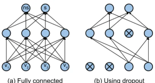
Neural networks are learning algorithms where inputs are fed through a series of layers comprised of units (also called neu-rons), where each unit has a non-linear activation function. An example fully-connected neural network, where the units in layermare connected to all of those in layerm − 1, is shown in Figure 1a. The hidden layers perform feature extraction by learning non-linear combinations of the inputs, where individu-ally the features may not be particularly descriptive [15]. Care must be taken when training neural networks as they are prone to overfitting on the training set if there is a lack of training ma-terial. In this section, the use of neural networks is described for predicting voicing classification of input 2D-DCT visual speech features. Two neural network models are trained,NN DCTfor static visual features, andNN DCT∆for visual features includ-ing temporal information.

2.1. Architecture

The network architecture used consists of a fully-connected net-work with a single hidden layer (consisting of 512 units) be-tween the input layer and output softmax layer. A softmax function is commonly used in the output layer for multiclass classification problems to ensure the values from the final ac-tivation functions lie in the range 0to 1, and that the sum of the values totals1, giving a categorical probability distribution. Using greater numbers of hidden layers—producing deep neu-ral networks—did not improve results enough to warrant the extra time required for training. The models are also relatively robust to the number of hidden units used, with values of256,

512, and1024, all producing comparable results.

Typical non-linear activation functions used in neural net-works are the tanh and sigmoid functions, which both saturate given large input values. The Rectified Linear Unit (ReLU) is a non-saturating activation function proposed by [16], and is cal-culated asf(x) =max(0, x). The benefit of building neural networks using ReLUs is that training concludes several times faster [11].

2.2. Dropout

Dropout [17] is a technique used in neural network architectures as a means to prevent overfitting of the training data. During training, neurons are selected at random and dropped. That is, the neuron and its connections are temporarily removed from the network for that particular instance or set of training exam-ples.

Figure 1a shows an example fully-connected neural

net-(a) Fully connected (b) Using dropout

ns s

v1 v2 v3 v4

Figure 1: A fully-connected network is shown in (a), and the same network after dropout has been applied in (b).

work with a single hidden layer. Figure 1b shows the same net-work after dropout has been applied. A probability ofp= 0.5

is typically used for dropout applied to fully-connected hidden layers, and a probability closer to zero for dropping input units. The effect of applying dropout during training is to train a num-ber of “thinned” models. For estimation, the classifications are then taken from the average of all the thinned-out networks. The effect is similar to training a large ensemble of models and av-eraging the predictions of each model [18].

2.3. Training

The neural networks are trained using the resilient backpropa-gation algorithm [19]. L2 regularization is applied with a value of0.001, and the learning rate is fixed at0.001. The training visual vectors are grouped into mini-batches of5000examples, withz-score normalisation applied to the input 2D-DCT visual features. Training is completed once validation scores converge.

3. Convolutional neural networks

Convolutional neural networks have shown application for myr-iad computer-vision tasks such as handwritten digit recognition, and are motivated by the function of the primary visual cor-tex [15]. Convolutional layers differ from fully-connected lay-ers (as shown in Figure 1a) in that the units in layermare con-nected to only a local subset (representing a “receptive field”) of the units in layerm − 1. Outputs from convolutional lay-ers are called feature maps, and are calculated by convolving the inputs with multiple square matrices, which are analogous to filter kernels as used for image edge detectors or blurring. Weight sharing of the kernels ensures that they can extract fea-tures independent of where they occur in the input.

Input Convolution Downsample Convolution Downsample Fully connected

Figure 2: Example convolutional neural network architecture with two convolutional and downsampling layers, connected to a final fully-connected output layer.

An example CNN architecture is shown in Figure 2. An input image is convolved with four kernels producing four fea-ture maps. A downsampling stage is performed following the convolution stage to reduce the size (width and height) of the feature maps. Max-pooling is used to perform this subsam-pling, whereby the maximum output of a small square window is taken. A further convolutional stage extracts eight feature maps, and is subsequently followed by another downsampling

layer. The output of the final subsampled layer is then input to a connected layer. Using deeper convolutional and fully-connected neural network architectures leads to the discovery of higher-level global features [20].

3.1. Architecture and training

The architecture used for this work follows Figure 2 and con-sists of two sets of convolutional–max-pooling–dropout layers, followed by a fully-connected hidden layer, and a final output softmax layer. The first convolutional layer consists of thirty-two filters of size 3×3, and the second, sixty-four filters of size3×3. Non-overlapping max-pooling follows each convo-lutional layer with square regions of size2×2. Dropout is then applied to each max-pooled layer with probabilityp= 0.2. The single fully-connected layer consists of512units, with dropout applied having probabilityp= 0.5. Rectified Linear Units are used throughout for activation functions.

Training is performed on an NVIDIA GRID K520 GPU card and takes approximately5h for the speaker dependent task and individual speaker independent runs. The visual frame pixel intensities are scaled to be in the range of zero to one, and train-ing is performed ustrain-ing mini-batches of size 50. The network is trained using Nesterov’s Accelerated Gradient Descent. Learn-ing rate annealLearn-ing is performed, decreasLearn-ing the value by1% per epoch, and training is completed once validation scores con-verge.

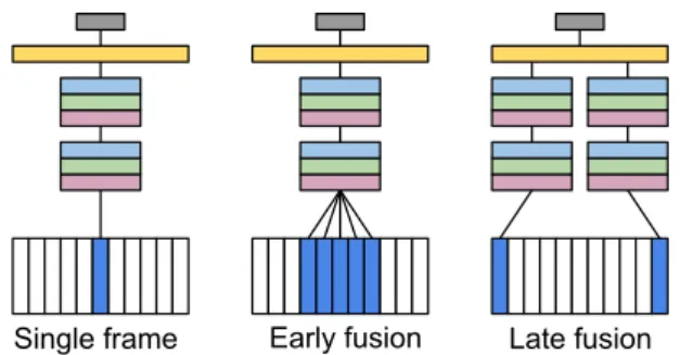
3.2. Temporal information

Deep neural networks, used for large-vocabulary speech recog-nition, include temporal information through the simple con-catenation of contiguous frames of audio features [9]. This ap-proach cannot be used directly with convolutional neural net-works at the input stage as the horizontal or vertical concatena-tion of frames would introduce issues at the boundaries of the images. An approach using early- and late-fusion for the inclu-sion of temporal information has shown success in large-scale video classification [12], and is applied here.

Single frame Early fusion Late fusion

Figure 3: Static frame, and early- and late-fusion CNN architec-tures for including temporal information. Blue frames denote those that have current interest.

Figure 3 shows the single frame, early-fusion, and late-fusion architectures, including the convolutional and fully-connected connections as shown in Figure 2. Early-fusion func-tions at the first layer, extending the depth of the first con-volutional layer filters to convolve across neighbouring video frames, for the detection of local motion direction. Late-fusion uses two separate convolutional columns for frames spaced a specific distance apart whose output is combined at the fully connected layers, therefore learning more global motion char-acteristics. However, the late-fusion technique is liable to miss

the more fine-grained mouth movements important for the tran-sitions between phones in the output audio speech. Experiments are conducted using a single frame system,CNN STATIC, and a system using the early-fusion technique to stack three neigh-bouring frames together, calledCNN STACK3.

4. GMM baseline system

In [5], GMMs are used to model visual feature vectors for voice activity detection, and this forms the baseline to compare the neural network and CNN systems against. Vectors are grouped by class label and individual GMMs are trained—Φs

for speech frames andΦns for non-speech frames. Classification is per-formed by taking thearg maxof the probabilities produced by each class GMM,Φl

, given the input visual vector,vt,

ˆ

cVADt = arg max l

p(vt|Φl)

, (2)

wherel∈ {ns, s}. Applying the system to the task of voicing classification requires the training of three GMMs, one each for non-speech frames, unvoiced frames, and voiced frames, result-ing in estimations given by,

ˆ cVCt = arg max l p(vt|Φl) , (3)

wherel ∈ {ns, u, v}. Through experimentation it was found that using sixteen clusters for each GMM gave the best per-formance. The two GMM models are namedGMM DCT and

GMM DCT∆, for the static and temporal models respectively.

5. Experiment description

Experiments are conducted on three systems for voicing classi-fication and voice activity detection. A baseline GMM system (see Section 4), a neural network system (see Section 2), and a novel convolutional neural network system (see Section 3). For the speaker dependent scenarios, experiments are conducted for all three systems with static features and when temporal in-formation has been added. For the speaker independent sce-nario, experiments are conducted on the GMM and neural net-work systems using first-order temporal derivatives, and on both CNN systems.

5.1. Dataset

The GRID audiovisual dataset [21] is used for the experiments. The dataset includes video of thirty-four speakers each hav-ing produced1000utterances. The videos are three seconds in length with twenty-five frames per second, giving seventy-five frames per video. The resolution of each frame is576×720

pixels, and contains RGB channel information. Word time-alignment files are included for each utterances that describes the start and end points for each word of the utterance, as well as periods of silence.

The speaker dependent task uses all visual data, totalling approximately 50 minutes, for the speaker (speaker6 in the corpus), and is split with80% for training and20% for test-ing. Data from nine speakers is used for the speaker indepen-dent task. One hundred utterances are selected from each of the nine speakers (speakers1–7,10, and12), therefore ensur-ing the trainensur-ing/testensur-ing data split is roughly equal for both the speaker dependent and independent tasks. k-fold cross valida-tion is used for the speaker independent experiments, segment-ing the trainsegment-ing data into that from eight of the speakers, and

then performing testing on the held-out speaker. This is re-peated for all permutations, and the final accuracy results are averaged.

5.2. Visual preprocessing

The video data is up-sampled to100Hz to match a typical audio speech frame rate of10ms. The FFMPEG suite of multimedia tools [22] is used to extract greyscale visual frames at the re-quired rate. Images of size96×96pixels are extracted about a centre-point of the mouth calculated from landmark data, and resized to64×64pixels. Figure 5a shows an example extracted mouth image.

Image-based visual speech features derived from a two-dimensional discrete cosine transform are used for the neural network and GMM systems. Features are extracted from a ma-trix of pixel intensities that is centred on a tracked mouth centre point. A 2D-DCT is applied to produce a coefficient matrix from which aJ-dimensional visual vector is obtained by ex-tracting coefficients in a zigzag order from the lower coefficient region of the matrix [23]. The first coefficient (the DC term) is discarded and 35 coefficients are retained.

5.3. Voicing classification labels

To measure voicing classification and voice activity detection accuracy, reference labels are required. Processing of the word time-alignment files is performed to provide VAD data, that is, the non-speech and speech classes.

cVADt = (

s ifx(t)is speech

ns otherwise (4) For the voicing classification task, labels are required for each frame of speech, t, classifying each as either non-speech, unvoiced, or voiced. The PEFAC pitch-extraction algo-rithm [24] is used to provide a probability that a given frame of speech is voiced. The voiced speech probabilities output from PEFAC are thresholded, with frames of speech having probabil-ityp(t)≥0.5labelled as voiced. Frames classified as speech using the voice activity data, described by Equation 4, that are not classified as voiced using PEFAC, are labelled as unvoiced.

cVCt =      v ifp(t)≥0.5 u if speech andp(t)<0.5 ns otherwise (5)

Equation 5 describes the class labels assigned to each frame. Median filtering is performed on the thresholded proba-bilities to remove isolated values.

6. Evaluation

In this section, accuracy results are presented for voicing classi-fication and voice activity detection of the three systems for the speaker dependent and speaker independent scenarios. Accura-cies are recorded for the multiclass voicing classification task, and then by grouping the unvoiced and voiced estimations, the VAD results are obtained. Lastly, intuition is given for the filter kernels learnt by the CNN systems and the convolutions they produce.

6.1. Speaker dependent results

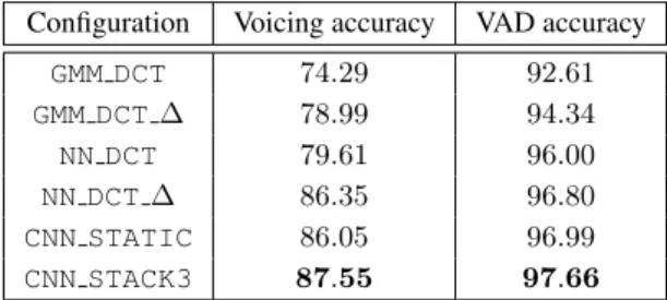
Table 1 shows voicing classification and voice activity detection accuracies for the speaker dependent task. TheCNN STACK3

achieves the best accuracy for voicing classification, with a score of87.55%. Accordingly, the same system outperforms both the GMM and neural network systems for voice activ-ity detection with an accuracy of 97.66%. Surprisingly, the

CNN STATICsystem is able to achieve86.05% voicing accu-racy using static information. In comparison, the static GMM and neural network systems achieve accuracies of11.76% and

6.44% lower respectively. This suggests that by using convo-lutional neural networks, suitably descriptive visual speech fea-ture representations can be found.

Table 1: Speaker dependent VAD and voicing classification ac-curacies in per cent.

Configuration Voicing accuracy VAD accuracy

GMM DCT 74.29 92.61 GMM DCT∆ 78.99 94.34 NN DCT 79.61 96.00 NN DCT∆ 86.35 96.80 CNN STATIC 86.05 96.99 CNN STACK3 87.55 97.66

Increased voicing classification accuracy by including tem-poral information is readily apparent for both the neural net-work and GMM systems. A classification accuracy increase of

4.7% and6.7% is gained for the GMM and neural network re-spectively. However, the same increase does not occur when using the CNN. Interestingly, it appears that due to the only slight increase in performance between theCNN STATICand

CNN STACK3 systems of1.5%, using the early-fusion tech-nique for including temporal information in the CNN architec-ture is not ideal for this work, and that other techniques for tem-poral fusion could result in a greater accuracy.

Table 2: Confusion matrix of per cent classification accuracy using theCNN STACK3speaker dependent model.

Non-speech Unvoiced Voiced Non-speech 98.23 1.49 0.28

Unvoiced 5.91 66.84 27.25

Voiced 0.72 8.93 90.36

Table 2 shows a confusion matrix for classification accu-racies for the speaker dependent CNN STACK3 model. The majority of voicing classification errors occur with the misclas-sification of unvoiced frames as voiced frames, with27.25% doing so. The problem experienced with voicing classification occurs when different voiced and unvoiced phonemes have the same visual speech realisations. Phonemes sharing the same vi-sual realisations can be grouped by phoneme equivalence class (PEC), a generalisation of the viseme for the grouping of visu-ally similar phonemes proposed by [25]. Regarding problems of voicing classification, a PEC comprised of /s t z/ consists of two unvoiced consonants, /s/ and /t/, and a voiced consonant, /z/, for example. A PEC comprised of /f v/ has a voiced and unvoiced consonant. The PECs described are taken from [26]. Voice activity detection errors can be seen where unvoiced or voiced frames are classified as non-speech, and vice versa. The problem in this case is that visual realisations of certain PECs have a mouth shape that is very visually similar to the neutral. For example, this is the case with the PEC comprised of the phonemes /b m p/. The majority of errors occur when unvoiced frames are misclassified as non-speech frames, happening for

5.91% of unvoiced frames.

6.2. Speaker independent results

The speaker independent results are displayed in Table 3. The

NN DCT∆system achieves accuracies of63.13% and78.69% for voicing classification and voice activity detection respec-tively, outperforming theGMM DCT∆system by11.02% and

8.19% for each task. The speaker independent results are con-siderably worse than the speaker dependent results, suggest-ing that greater attention needs to be spent on removsuggest-ing visual speech feature differences existing between speakers.

Table 3: Speaker independent VAD and voicing classification accuracies in per cent.

Configuration Voicing accuracy VAD accuracy

GMM DCT∆ 52.11 70.50

NN DCT∆ 63.13 78.69

CNN STATIC 59.02 74.07

CNN STACK3 59.02 74.68

The CNN systems do not perform as well for the speaker independent scenario. The best system, CNN STACK3, us-ing temporal information, achieves accuracies of59.02% and

74.68% for voicing classification and VAD. There is also not a noticeable difference between the static and temporal models, which again suggests that other methods of including tempo-ral information in the convolutional neutempo-ral network architecture would increase results.

Table 4: Confusion matrix of classification accuracies in per cent for speaker one using theCNN STACK3speaker indepen-dent model.

Non-speech Unvoiced Voiced Non-speech 90.58 8.94 0.47

Unvoiced 34.70 54.80 10.50

Voiced 14.58 43.98 41.44

Table 4 shows a confusion matrix for classification accura-cies for speaker one trained on the other eight speakers using theCNN STACK3system. In comparison to Table 2, it can be seen that the majority of voicing classification errors come from an increase in voiced frames being misclassified as unvoiced, and from unvoiced frames being misclassified as non-speech. In terms of voice activity detection, there is a large increase in the number of unvoiced and voiced frames that are misclassified as non-speech.

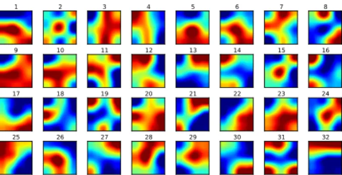
6.3. Visualisation of learnt filters and convolutions

Visualisations of the thirty-two 3×3filter kernels learnt by the first convolutional layer are shown in Figure 4. The kernel values have been resized (using cubic interpolation) and nor-malised in the range of zero to one for display. A variety of the learnt kernels show edge detection properties. For example, kernels17and32highlight horizontal edges, whereas kernels

22and25highlight diagonal edges.

As shown in Figure 2, the result of convolving an input im-age with the filter kernels is to produce a number of feature maps. Figure 5a shows an original mouth image as would be input to the CNN, and a selection of feature maps after con-volution with the kernels. Concon-volutions with kernels2and32

1 2 3 4 5 6 7 8

9 10 11 12 13 14 15 16

17 18 19 20 21 22 23 24

25 26 27 28 29 30 31 32

Figure 4: Thirty-two kernels learnt in the first convolutional layer for the speaker dependent task. Blue values are lower, red are higher.

(see Figures 5b and 5d) serve to highlight the area of the inner mouth, effectively removing information of the skin and lips, with kernel2exhibiting more blurring than kernel32. The im-age convolved with kernel25(see Figure 5c) shows how the diagonal edges have been highlighted, as can be seen by the greater pixel intensity on the upper-left edges of the teeth, and in the lower-right corner of the inner mouth.

(a)

Original

2

25

32

Figure 5: Example original mouth image, and when convolved with filter kernels2,25, and32, as depicted in Figure 4.

7. Conclusion

For the speaker dependent scenario the novel convolutional ral network approach outperforms the baseline GMM and neu-ral network systems for both voicing classification and voice activity detection. The high accuracy achieved for the CNN us-ing static information shows promise for their ability to discover descriptive visual speech feature representations. As such, their use in current audiovisual VADs for the visual stream should prove beneficial. Similarly, their use in other applications, such as lip reading and audiovisual automatic speech recognition, could improve accuracy for speaker dependent scenarios. A further increase in accuracy for voicing classification could be attained by better incorporating temporal information into the system.

The neural network outperforms both the GMM and CNN systems for the speaker independent scenario, presumably as the hidden layer feature extraction can better ignore the between-speaker differences. Further work on removing the differences between visual speech features of different speakers would, therefore, likely increase the speaker independent results achieved. Regarding the convolutional neural networks, explor-ing different architectures in depth, the application of state-of-the-art techniques, and a large increase in the amount of speaker training data used, should all serve to increase accuracy.

8. References

[1] J. Ramırez, J. C. Segura, C. Benıtez, A. De La Torre, and A. Ru-bio, “Efficient voice activity detection algorithms using long-term speech information,”Speech communication, vol. 42, no. 3, pp. 271–287, 2004.

[2] Q. Summerfield, “Some preliminaries to a comprehensive ac-count of audio-visual speech perception,” in Hearing by Eye:

The Psychology of Lip-Reading, B. Dodd and R. Campbell, Eds.

Lawrence Erlbaum Associates, 1987.

[3] S. Dupont and J. Luettin, “Audio-visual speech modeling for con-tinuous speech recognition,”Multimedia, IEEE Transactions on, vol. 2, no. 3, pp. 141–151, 2000.

[4] P. Liu and Z. Wang, “Voice activity detection using visual infor-mation,” inAcoustics, Speech, and Signal Processing, 2004.

Pro-ceedings.(ICASSP’04). IEEE International Conference on, vol. 1.

IEEE, 2004, pp. I–609.

[5] I. Almajai and B. Milner, “Using audio-visual features for robust voice activity detection in clean and noisy speech,” inProc.

EU-SIPCO, vol. 86, 2008.

[6] A. Aubrey, B. Rivet, Y. Hicks, L. Girin, J. Chambers, and C. Jut-ten, “Two novel visual voice activity detectors based on appear-ance models and retinal filltering,” in15th European Signal

Pro-cessing Conference (EUSIPCO-2007), 2007.

[7] D. Sodoyer, B. Rivet, L. Girin, J.-L. Schwartz, and C. Jutten, “An analysis of visual speech information applied to voice activ-ity detection,” inAcoustics, Speech and Signal Processing, 2006. ICASSP 2006 Proceedings. 2006 IEEE International Conference on, vol. 1. IEEE, 2006, pp. I–I.

[8] A. Aubrey, Y. Hicks, and J. Chambers, “Visual voice activity de-tection with optical flow,”IET image processing, vol. 4, no. 6, pp. 463–472, 2010.

[9] G. Hinton, L. Deng, D. Yu, G. E. Dahl, A.-r. Mohamed, N. Jaitly, A. Senior, V. Vanhoucke, P. Nguyen, T. N. Sainathet al., “Deep neural networks for acoustic modeling in speech recognition: The shared views of four research groups,”Signal Processing Maga-zine, IEEE, vol. 29, no. 6, pp. 82–97, 2012.

[10] G. E. Dahl, T. N. Sainath, and G. E. Hinton, “Improving deep neu-ral networks for LVCSR using rectified linear units and dropout,”

inAcoustics, Speech and Signal Processing (ICASSP), 2013 IEEE

International Conference on. IEEE, 2013, pp. 8609–8613.

[11] A. Krizhevsky, I. Sutskever, and G. E. Hinton, “ImageNet classi-fication with deep convolutional neural networks,” inAdvances in

neural information processing systems, 2012, pp. 1097–1105.

[12] A. Karpathy, G. Toderici, S. Shetty, T. Leung, R. Sukthankar, and L. Fei-Fei, “Large-scale video classification with convolutional neural networks,” inComputer Vision and Pattern Recognition

(CVPR), 2014 IEEE Conference on. IEEE, 2014, pp. 1725–1732.

[13] T. N. Sainath, A.-r. Mohamed, B. Kingsbury, and B. Ramabhad-ran, “Deep convolutional neural networks for LVCSR,” in Acous-tics, Speech and Signal Processing (ICASSP), 2013 IEEE

Inter-national Conference on. IEEE, 2013, pp. 8614–8618.

[14] O. Abdel-Hamid, L. Deng, and D. Yu, “Exploring convolutional neural network structures and optimization techniques for speech recognition.” inINTERSPEECH, 2013, pp. 3366–3370. [15] K. P. Murphy, Machine learning: a probabilistic perspective.

MIT press, 2012.

[16] V. Nair and G. E. Hinton, “Rectified linear units improve restricted boltzmann machines,” inProceedings of the 27th International

Conference on Machine Learning (ICML-10), 2010, pp. 807–814.

[17] N. Srivastava, G. Hinton, A. Krizhevsky, I. Sutskever, and R. Salakhutdinov, “Dropout: A simple way to prevent neural net-works from overfitting,”The Journal of Machine Learning

Re-search, vol. 15, no. 1, pp. 1929–1958, 2014.

[18] I. J. Goodfellow, D. Warde-Farley, M. Mirza, A. Courville, and Y. Bengio, “Maxout networks,”arXiv preprint arXiv:1302.4389, 2013.

[19] M. Riedmiller and H. Braun, “A direct adaptive method for faster backpropagation learning: The RPROP algorithm,” inNeural

Net-works, 1993., IEEE International Conference on. IEEE, 1993,

pp. 586–591.

[20] Y. Sun, X. Wang, and X. Tang, “Deep convolutional network cas-cade for facial point detection,” inComputer Vision and Pattern

Recognition (CVPR), 2013 IEEE Conference on. IEEE, 2013,

pp. 3476–3483.

[21] M. Cooke, J. Barker, S. Cunningham, and X. Shao, “An audio-visual corpus for speech perception and automatic speech recog-nition,” The Journal of the Acoustical Society of America, vol. 120, no. 5, pp. 2421–2424, 2006.

[22] “FFmpeg,” https://www.ffmpeg.org/, accessed: 28/04/2015. [23] K. Sayood, Introduction to data compression.

Morgan-Kaufmann, 2000.

[24] S. Gonzalez and M. Brookes, “PEFAC-a pitch estimation algo-rithm robust to high levels of noise,” Audio, Speech, and

Lan-guage Processing, IEEE/ACM Transactions on, vol. 22, no. 2, pp.

518–530, 2014.

[25] E. T. Auer Jr and L. E. Bernstein, “Speechreading and the struc-ture of the lexicon: Computationally modeling the effects of re-duced phonetic distinctiveness on lexical uniqueness,”The Jour-nal of the Acoustical Society of America, vol. 102, no. 6, pp. 3704– 3710, 1997.

[26] L. Bernstein, “Visual speech perception,” AudioVisual Speech