A Personalized Recommender System with Correlation Estimation

(1)

A Personalized Recommender System with Correlation

Estimation

A THESIS

SUBMITTED TO THE FACULTY OF THE GRADUATE SCHOOL OF THE UNIVERSITY OF MINNESOTA

BY

Fan Yang

IN PARTIAL FULFILLMENT OF THE REQUIREMENTS FOR THE DEGREE OF

Doctor of Philosophy

Xiaotong Shen

(2)

c

Fan Yang 2018

(3)

Acknowledgements

First and foremost, I would like to take this opportunity to express my greatest ap-preciations to my thesis advisor Prof. Xiaotong Shen. Over the years, he has been generously sharing his time and knowledge, and offering me invaluable advice in both my academic research and personal development. I’m deeply grateful and honored to be influenced by his insights and professionalism. It is his constant support, help, and patience for various aspects of my life that made this work possible.

I would also like to thank the rest of my committee members, Prof. Charles Geyer, Prof. Adam Rothman and Prof. Wei Pan. I’m grateful to have them as my committee members and I deeply appreciate their guidance and words of encouragement along the way.

I’m also grateful to my friends at the University of Minnesota for making the expe-rience here enjoyable. Thanks go to Yunzhang Zhu, Yiping Yuan, Qi Yan, Zhihua Su, Feng Yi, Ben Sherwood, Yiwen Sun, Yuwen Gu, Yanjia Yu, Bo Peng, Dootika Vats, Subhabrata Majumdar, Xuetong Sun and many other friends in the Stat department, as well as my friends in other departments.

My special thanks go to my mother and my sister, who loved me and supported me all the time.

Finally, thank Jun for being by my side. I’m grateful to have you joining my life and thank you for all your love and support.

(4)

Dedication

To the memory of my father Cuizhen Yang and To my mother Xinrong Li.

(5)

Abstract

Recommender systems aim to predict users’ ratings on items and suggest certain items to users that they are most likely to be interested in. Recent years there has been a lot of interest in developing recommender systems, especially personalized rec-ommender systems to efficiently provide personalized services and increase conversion rates in commerce. Personalized recommender systems identify every individual’s pref-erences through analyzing users’ behavior, and sometimes also analyzing user and item feature information.

Existing recommender system methods typically ignore the correlations between ratings given by a user. However, based on our observation the correlations can be strong. We propose a new personalized recommender system method that takes into account the correlation structure of ratings by a user. General precision matrices are estimated for the ratings of each user and clustered among users by supervised clustering. Moreover, in the proposed model we utilize user and item feature information, such as the demographic information of users and genres of movies. Individual preferences are estimated and grouped over users and items to find similar individuals that are close in nature. Computationally, we designed an algorithm applying the difference of convex method and the alternating direction method of multipliers to deal with the nonconvexity of the loss function and the fusion type penalty respectively. Theoretical rate of convergence is investigated for our new method. We also show theoretically that incorporating the correlation structure gives higher asymptotic efficiency of the estimators compared to ignoring it. Both simulation studies and Movielens data indicate that our method outperforms existing competitive recommender system methods.

(6)

List of Tables

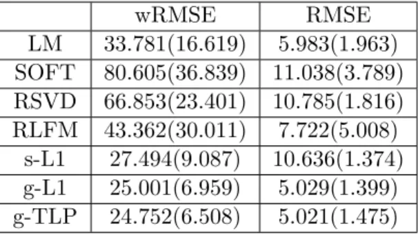
4.1 Simulation results for seven methods are reported: LM is the linear re-gression model using rating as the response and user and item features as predictors; SOFT is the SOFT-IMPUTE method; RSVD is regular-ized singular value decomposition; s-L1 is specialL1 clustering ignoring precision matrix; RLFM is the regression-based latent factor model; g-L1 is the generalL1 clustering (considering precision matrix); g-TLP is the general TLP clustering (considering precision matrix). Numbers in the parentheses are the standard errors. . . 55 4.2 Movielens 100k RMSE with seven methods: LM is the linear regression

model using rating as the response and user and item features as pre-dictors; SOFT is the Soft-Impute method; RSVD is regularized singular value decomposition; RLFM is the regression-based latent factor model; s-L1 is specialL1clustering ignoring precision matrix; g-L1 is the general L1 clustering (considering precision matrix); g-TLP is the general TLP clustering (considering precision matrix). . . 57

(9)

List of Figures

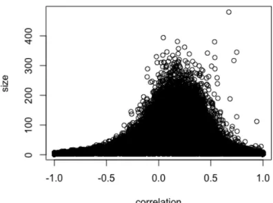
2.1 SVD in recommender systems1 . . . 10 5.1 Correlation of two movie ratings . . . 85 5.2 Sample size v.s. correlation . . . 86

(10)

Chapter 1

Introduction

Recommender Systems are used to predict users’ response to options/items. With the development of the internet, recommender systems are becoming more and more impor-tant. They are applied very widely to e-commerce, including recommending restaurants, hotels, news, mobile phone games, movies and so on. For example, Netflix recommends movies based on history ratings and movie rental information; Expedia recommends hotels to book based on history information. Online retailers like Amazon.com and ebay.com which sell a vast variety of goods and services also take advantage of rec-ommender systems to sell their products. Amazon and eBay recommend items by suggesting new lists like “More Items to Consider” and “Customers Who Bought This Item Also Bought” etc.

Generally, the problem of recommender systems is for a given user, to recommend some items this user is likely to be interested in. There are many specific formats of recommender systems designed for data collected from different recommendation scenarios.

Some recommendation applications inquire the user’s conditions or criteria before they give recommendations thus they require the user to interact with the system in order to provide a recommendation. For example, on yelp.com users can specify the city they want to search, the price they would like to pay (divided to 4 price levels), the neighborhoods, distance, features (breakfast, brunch etc.), style of meals (American, Chinese etc.), and then get recommendations that meet their needs. This kind of recommender system which depends on knowledge about the user’s needs and also

(11)

about the products is known as knowledge-based recommender systems [8].

Other recommender systems do not ask the user to input their needs and require-ments for the next recommendation. They only use what is already in the system such as history ratings of users on other items. The systems may also collect user demographic information such as age and gender, and item feature information. These recommender systems typically aim at predicting the rating of an item a user has not purchased or seen before, using the information available. After the predictions are generated, items with the highest predicted ratings are recommended to users. There are also recommender systems that target at predicting ranking of unrated items, such as the rankboost algo-rithm proposed in [21]. They care about the relative orders of products and recommend items with the lowest ranking. We focus on these types of recommender systems which don’t ask user needs for next item because they require less involvement of users and is applicable to most practical recommendation problems. This is also the most widely known and most commonly used formulation of recommender systems.

Recommender systems that predict ratings are the most commonly used format of all recommender systems, and we are mainly talking about this kind of recommenders in this introduction. The framework can be stated as follows. Suppose we have nusers and m items. Let rij be the rating of user i on item j. Then all the ratings can be written in a matrix R= (rij), with some question marks to represent unknown ratings.

R=           r11 r12 ? . . . r1m ? r22 r23 . . . ? r31 ? ? . . . r3m .. . ... ... . .. ... ? ? rn3 . . . ?           , (1.1)

where each row is the ratings of one user, and each column is the ratings on one item. In recommender systems, only part of the matrixR is observed. The entryrij is observed if userihas rated itemj, and not observed otherwise. Usually there are a huge number of items, and users only rated a few of them. So a very large proportion ofRis missing. We want to predict the missing ratings accurately.

(12)

science literature since collaborative filtering recommender systems appeared in the mid-1990s [1]. Afterwards a lot of developments were made in both industry and academia. Currently, there are two prevalent classes of approaches, i.e. collaborative filtering and content-based recommender systems. Collaborative filtering makes use of the informa-tion from similar users to predict the future acinforma-tion. Popular methods include matrix factorization approaches such as SVD decomposition in [22, 30] and many variants, matrix completion approaches such as [34].

Content-based recommender systems (e.g. [12, 7]) compare the content of an item with a user’s profile and are mostly used in recommending textual materials. Techniques such as TF-IDF [45] in information retrieval are utilized for item feature extraction. One advantage of content-based methods is that ratings on new items can be predicted which solves the “cold start” problem partially. There are also many hybrid recommender systems developed combining collaborative filtering and content-based methods, for example [44, 3, 64]. Context-aware recommender systems which take into account the context under which a user rates an item have also been introduced, such as in [28] and [5]. Hybrid and context-aware methods have become the trend in recommender systems.

The existing methods typically assume the ratings of a given user on different items are independent, and ignore the missing mechanism of R which is usually not missing completely at random. The method in [6] takes one step further: they proposed a group-specific singular value decomposition method, by clustering users or items according to a certain missing mechanism they observed. Hence their method captures the individuals’ latent characteristics that are not used in other approaches, and provides more accurate prediction than the previously mentioned methods. These will be explained with more details in Chapter 2.

We propose a correlation-incorporated method, which takes one step further than the typical methods, along a different direction from [6]. We notice that a user’s rating on different items could be highly correlated: in the MovieLen data, this is extraordi-narily apparent for different episodes of a movie series (Star Wars, for example); and this is also obvious for different movies adopted from similar true stories or related lit-erary works. In nowadays cyber-context, there is some phenomenon called Intellectual Property (IP). Many movies can root from the same IP, and if this IP is particularly

(13)

preferred or disliked by a certain user, it is expected that such a user will rate these different movies in a highly correlated way. This IP phenomenon is one evidence for us to consider the correlation of ratings over different items, for further discussion see section 3.4. Note that these correlations cannot be captured by the explicit feature or latent characteristics. Inspired by this observation, we take the precision matrix into consideration in our method.

Another motivation for considering the precision matrix is that we have a grouping of users, according to their correlations. Our method of estimating the precision matrix generalizes the method of [63], which automatically gives the grouping by fused type penalty. Furthermore, we combine this grouping by taking into account user preference on item features and item “preference” on user features. Also the grouping is auto-matically given through our algorithm. Note that estimation the of precision matrix together with the preference vectors requires a large amount of computation, and we can reduce the effort by the above-mentioned grouping. Moreover, the incorporation of the correlation structure is proved to deliver smaller asymptotic variance and prediction error theoretically, thus increases the accuracy of the method.

The structure of the rest of this thesis is as follows: Chapter 2 is literature review about state of the art recommender systems; Chapter 3 discusses about the statistical model we propose, algorithm and theoretical results; Chapter 4 shows our numerical results in simulations and Movielens dataset; Chapter 5 gives a conclusion and discussion of our method.

(14)

Chapter 2

Four Kinds of Recommender

Systems

There are some very challenging problems to solve in recommender systems. In most real applications, the number of users and items are both huge. For example, Amazon.com currently has about 300 million active customers and sells over 400 million products. With such a large dataset, fast computation inevitably becomes an issue. Scalability of the algorithm is necessary in order for it to be used in recommender systems to solve practical problems. Another challenge is that, although there are a huge number of users and items, the number of items rated by a user takes up a very small proportion of all items, usually below 1%. This makes it hard to predict unknown ratings precisely. It can be easily imagined this is the case for Internet companies like Amazon.com or Netflix as they have so many items. In research, the movie recommendation problem is studied quite often because of the availability of datasets in the public domain. This practical problem also has the issue of extremely low percentage of observed ratings. The popular Movielens dataset is provided by GroupLens, a research lab which studies recommender systems and some other related areas at the University of Minnesota. It contains three movie rating data of 100k, 1M and 10M, and the average proportions of rated movies among all movies in these three datasets are 6.3%, 4.2% and 1.3% respectively.

According to what information is used for predicting ratings, recommender systems

(15)

can be classified into several kinds (here we again ignore knowledge-based recommender systems which don’t predict ratings). They are listed below and the basic idea is stated here.

• Collaborative Filtering recommender systems

This kind of recommender systems utilizes user history rating information. Similar users are found by similar ratings, and their ratings are aggregated for prediction. This allows preference of other users to be borrowed when predicting a user’s rating on an item not consumed by him/her before.

• Content-Based recommender systems

This kind of recommender systems utilizes item contents or features. Similar items are found by similar contents, and ratings on them are aggregated for prediction.

• Hybrid recommender systems

This kind of recommender systems seek ways to combine collaborative filtering and content-based recommender systems. Thus they utilize both user history ratings and item content information.

• Context-Aware recommender systems

As suggested by its name, this kind of recommender systems is aware of the context where the recommendation is made, for example what time the user consumes the item, or whether there is a companion. So context is an extra dimension considered besides user history ratings and item contents by context-aware recommender systems.

The following sections in this chapter are going to explain each of them in detail.

2.1 Collaborative Filtering

Collaborative filtering recommender systems are the earliest developed recommender systems. They appeared in the mid-1990s. The earliest works are [43, 24, 49]. Collabo-rative filtering utilizes the partially filled rating matrixRin (1.1). To predict for a user, rather than only using ratings of this user, collaborative filtering believes there is some

(16)

latent connection between all users and items and thus pools available information from all users on all items together in some way. Traditional collaborative filtering methods directly find similar users based on past ratings on common items. Recent collaborative filtering methods don’t define an explicit similarity measure but implicitly infers user relations. This way it’s more flexible and doesn’t only depend on one metric between users. Below they are discussed in more detail. An extensive review can be found in [10].

2.1.1 Traditional Collaborative Filtering

Traditional collaborative filtering recommender systems are based on the idea that peo-ple who share the same preferences in the past should also have the same preferences in the future. Given history ratings, similar users can be found as the ones who gave the closest ratings on the commonly rated items. Then the ratings of a user can be predicted based on the ratings of his/her similar users using a weighted or unweighted average. To be specific, following the notations in the Introduction chapter, suppose useriratedmi items. Denote the indices of items user irated by Ii,{i1,i2,· · · , imi} ⊆ {1,2,· · · , m}. For every other users, we calculate the similarity with user ibased on their ratings on items they both rated. Let Iij ={k|k∈Ii and k ∈Ij}. The two most commonly used similarity measures are the cosine and correlation measure.

sim1(i, j) = P k∈Iij rikrjk r _P k∈Iij r2 ik r _P k∈Iij r2 jk (cosine) sim2(i, j) = P k∈Iij (rik−ri)(rjk−rj) r P k∈Iij (rik−ri)2r P k∈Iij (rjk −rj)2 (correlation) (2.1) In above,ri = P k∈_Iij rik |Iij| and rj = P k∈_Iij rjk |Iij| .

Besides cosine and correlation similarities, many other measures can be used. For example as described in [49], inverse of distance measures such as mean squared dif-ference. There are also variants of the cosine and correlation similarities such as the

(17)

constrained Pearson correlation in [49] which takes into account the positivity and nega-tivity of ratings. Its idea is as follows. Many of the rating system adopt possible ratings as consecutive integers. For instance, if the ratings are in 1,2,· · · , s, then (s+ 1)/2 is the middle rating. Ratings greater than or equal to (s+ 1)/2 are positive, and smaller than (s+1)/2 are negative. If only ratings that are both positive or negative are allowed to increase the similarity, then a similarity measure can be

sim3(i, j) = P k∈Iij rik− s+ 1 2 rjk− s+ 1 2 s P k∈Iij rik−s+ 1 2 2 s P k∈Iij rjk−s+ 1 2 2 . (2.2)

Given similarities between user iwith all the other users, the K nearest neighbors can be used to predict ratings on items not rated by useriyet, whereKis a pre-specified integer. when K = n−1, it’s all users. Of course, when predicting user i’s rating on item l, only users who rated this item will be used. After the users are fixed, either a weighted or unweighted rating of these users can be calculated as the predicted rating for user i. If weights are used, they are usually based on the similarities. To present it, let U be the set of users used for predicting rating on item lof useriwhich isril. Some examples of averaging ratings are

1. rilˆ = P j∈U rjl |U| (Unweighted average) 2. rilˆ = P j∈U sim(i, j)·rjl P j∈U

sim(i, j) (Weighted average)

(2.3)

There are also many other ways to average ratings. For example, to account for the fact that different users may have different mean ratings, the ratings can be aggregated

(18)

as 3. rilˆ =ri+ P j∈U (rjl−rj) |U| (Unweighted average) 4. rˆil=ri+ P j∈U sim(i, j)·(rjl−rj) P j∈U

sim(i, j) (Weighted average)

(2.4)

The above methods to do collaborative filtering are the “traditional” methods and the algorithms are quite intuition-based. They are easy to implement but if users don’t share many rated items, then similarities are not accurate and thus affect the accuracy of prediction.

2.1.2 Recent Collaborative Filtering

Many advanced methods have been developed for collaborative filtering. [35] described a user-based and an item-based naive Bayes classifier. The user-based classifier treats the rating of one user as the response, and ratings of other users as features. It assumes given the rating of one user, ratings of all other users are independent. A posterior probability of this user’s rating given all other user ratings can be calculated and used for prediction. The item-based classifier is a similar idea.

Another popular approach is via matrix decomposition/completion. The Singular Value Decomposition (SVD) is applied in recommender systems to reduce the dimension of user and item feature space as well as approximating the history ratings [46, 30, 32]. Specifically, the rating matrix Rn×m is decomposed into the product of two low-rank matricesAn×k andBm×k while minimizingkR−ABTk22. The column dimensionkfor A and B satisfykmin{m, n}.

(19)

Figure 2.1: SVD in recommender systems1

AandB can be understood as the latent user and item factors that influences final ratings.

If R is a complete matrix, then the solution ofA and B will be the SVD of R by taking the firstksingular values. But sinceRis not complete, the minimization is done on the observed entries:

( ˆA,B) = argminˆ

A,B

X

(i,j)∈O

(rij−aTi bj)2, (2.5)

where O is the set of observed ratings, andai and bj are the ith andjth row of Aand B respectively. A regularized form of (2.5) is

( ˆA,B) = argminˆ A,B X (i,j)∈O (rij −aTibj)2+λ( n X i=1 kaik22+ m X j=1 kbjk22), (2.6)

whereλ >0 is a regularization constant. The above shrinksAandBtowards 0 to avoid overfitting. Alternating least squares algorithm can be used to solve (2.6), in which A and B are minimized alternately.

The method in [34] proposed to solve the following matrix completion problem for recommender systems: ˆ Z= argmin Z X (i,j)∈O (rij−zij)2+λkZk∗. (2.7)

Here Z is an×mmatrix. kZk∗ is the nuclear norm (also known as trace norm) which 1_{Stanford CS 294-34 slides}

(20)

is defined as kZk∗= n X i=1 σi, (2.8)

where the σi’s are the singular values of Z. The nuclear norm is used as a convex relaxation of rank. [34] also gave an efficient algorithm based on SVD to solve the above optimization.

Other people have proposed regularizing different matrix norms for the matrix com-pletion. For example, the local max norm used in [20].

Rendle 2010 [41] proposed a new model class of factorization machine which can be applied to predict ratings. FMs model all the main terms and interactions of the input features. Parameters for the interaction terms are estimated through factorization. This allows coefficients to share components, and works well in sparse data setting such as recommender systems. The model equation is

ˆ y(x) =w0+ X i wixi+ X i,j <vi,vj > xixj, (2.9)

where w0,w,V are parameters to estimate, andx is the input covariates for the corre-sponding response variable y. For example wheny=rij, the rating of userion itemj, then x can be a vector of indicator variables with the first part as n−1 indicators to index the user, and the second part as m−1 indicators to index the item. If available, the user and item feature vectors can also be incorporated inx, which makes it a hybrid recommender system.

Collaborative filtering recommender systems commonly have the new user and new item problem. For a new user entering the system, since no history rating is available, the system cannot make predictions for this user. Also for a new item which nobody has rated before, the system cannot predict ratings on it.

2.2 Content-Based Recommender Systems

Content-based recommender systems utilize the item features. The basic idea is users will like items similar to what they liked in the past. It doesn’t combine information

(21)

across users. Current content-based recommender systems are mostly used in applica-tions recommending items that contain texts such as web pages, documents [1], where the feature of the item is abundant enough to reflect the user preference.

Given the features of two items, say pi and pj respectively for item i and j, the similarity of these two items can be calculated using measures such as the cosine and correlation similarities given in (2.1). For example, the cosine similarity is

sim(itemi,itemj) = pi·pj

kpik2· kpjk2

. (2.10)

Then the predicted rating on an item can be decided by using the ratings on its nearest neighbors, such as using the unweighted or weighted average as in (2.3), (2.4).

In content-based recommender systems, since user preference is represented by the items rated in the past, how to extract informative features is an important issue. Recent advancements in information retrieval provides effective ways to extract features from textual contents. Typically texts are represented by its keywords. The simplest way is to count the times a word appears in the text. A more advanced and well-known approach to measure the importance of a word in a text is the TF-IDF (term frequency/inverse document frequency) measure [7, 45]. For keyword t, suppose it appears in documentd forft,d times, then its TF (term frequency) can be defined in several formats including but not limited to

TF(t, d) =ft,d, TF(t, d) = ft,d max s fs,d , TF(t, d) = 1 + log(ft,d). (2.11)

The IDF factor accounts for the fact that a keyword is not important if it appears in many documents. Suppose keywordtappears inmddocuments among allmdocuments. To make it clear, denote the collection of all documents by D. Then the IDF (inverse document frequency) and some of its variants are

(22)

IDF(t, D) = log m md, IDF(t, D) = log 1 + m md , IDF(t, D) = log 1 + max d md md ! . (2.12)

And the TF-IDF weight is the product of TF and IDF:

TF-IDF(t, d) = TF(t, d)·IDF(t, D). (2.13)

Let wt,d be the weight of keyword t in document d. After all keyword weights are derived, each document can be represented by the weights . Use wd to represent the profile/feature vector of documentd,

wd= (w1,d, w2,d,· · ·, wT ,d)T. (2.14) Some content-based recommender systems build a user interest profile for each user. The user profile is based on the keyword weight vectors wd’s of documents rated by the user. A typical way is to use a weighted average of wd’s weighted according to the ratings. Then prediction on new items is made by comparing the user profile and the keyword weight vector of the new item. Items with high keyword similarities to the user profile are predicted to have high ratings and items with low keyword similarities are predicted to have low ratings.

Besides using the nearest neighbor type of approach, other techniques are applied to content-based recommender systems. Naive Bayes can be applied assuming the features are independent of each other given the rating. Machine learning methods such as decision trees, random forest and neural network can also be applied.

As item feature is of essential importance to content-based recommender systems, one limitation of content-based recommender systems is that it may not perform well if the features cannot represent the item sufficiently. Even for texts where effective ways of extracting features are available from information retrieval field, there is still a concern whether keywords alone is sufficient to describe a text. That’s because even if

(23)

two documents use almost the same words, the way the words are organized can still be different. This is related to the writing style or quality of the document. Currently there’s no valid methods to capture this aspect of texts. For non-textual items such as videos and images, automatic feature extraction still remains a problem. For example in movie recommendation, features such as the director, time of release, genre and so on can be obtained, but the movie video itself cannot be parsed and thus gives no features at all. With such limited features, content-based recommender systems may not learn the preferences of users well to give accurate predictions.

Another drawback of content-based recommender systems is that content-based sys-tems can only recommend isys-tems similar to the ones rated before. Isys-tems dissimilar have a low similarity score and the predicted rating will be low. So they are always ignored and never get recommended to the user. But in fact, users are possible to select dif-ferent items which are not similar to the previous ones next time. Thus content-based recommender systems limit user interests to the old ones and give too low ratings to dissimilar items.

Content-based recommender systems also have the new user problem, as collabora-tive filtering systems. For a new user who hasn’t rated any item yet, a content-based system cannot learn his/her preferences. So no prediction can be made for this user. But different from collaborative filtering, content-based systems do not have the new item problem. The system doesn’t rely on ratings of other people to predict for one user. It only relies on the “content” of the item. So even though no one has rated this item, based on the similarity of this item with the rated ones, the rating on this item can still be predicted.

2.3 Hybrid Recommender Systems

In many applications, both the user history rating information and item feature infor-mation can be obtained. Thus only using history ratings or only using item features is not efficient. A hybrid recommender system combining collaborative filtering which uses history ratings and content-based recommender systems which use item features can perform better. Furthermore, combining these two types of recommender systems can avoid the problems specific to one of them.

(24)

There are many ways to combine the two types of recommender systems. Hybrid recommender systems can be categorized into three classes [1, 9].

1. Use both collaborative filtering and content-based recommender system to predict the ratings. The ratings from these two systems are combined in some way.

2. Augment the feature space of one system from features in the other system.

3. Build a unified model that use both user history ratings and item features.

Details and some examples of three types of hybrid recommender systems are given below.

2.3.1 Combining Results and Augmenting Feature Space

Directly combining results is the most straightforward way of combining collaborative filtering and content-based recommender systems. To fulfill this, first both methods are implemented. To combine them, the simplest way is to do a linear combination. In real applications, the weights of two systems are often adjusted as more prediction are made and performance are seen. For example one possibility is to use equal weights at the beginning. As more predictions are made, the weight of the system that gives ratings closer to the observed gets larger, and the other weight gets smaller. Another approach used is switching between the two systems using some criteria. For example, the DailyLearner system tries content-based recommender system first. If it doesn’t have high confidence in the predicted rating, then collaborative filtering is implemented and used.

An example of augmenting feature space can be to modify the similarity score calcu-lation for two users in the traditional collaborative filtering system. To incorporate item feature information, for a user the history ratings can be augmented by the user profile built in a content-based recommender system. To be specific, suppose the user history ratings are in vector ri, and the user profile iswi. Then the augmented representation of this user is (all vectors are column vectors)

(25)

And the similarity score between users can be calculated based on rwi’s. For user i and j, ri and rj are ratings on items they both rated. In cases where the number of commonly rated items is small for a pair of users, only using ratings to compute similarity may not give an accurate measure. The augmentation of item features can relieve this issue by adding more elements to the base of the comparison.

2.3.2 Building a Unified Model

Many recently developed hybrid recommender systems do not combine the result from the two methods or augment the features, like in section § 2.3.1. Instead, they utilize user history ratings and item features at the beginning step of the model building. Some examples of them are given below.

A unified probabilistic model was proposed in [47]. It builds a distribution over all user and movie pairs. The probability of user ipurchase/rate item j is modeled using a latent class for users. Item content information is also incorporated to model the probability.

In [44] another probabilistic model was proposed. It employed the Restricted Boltz-mann machines to combine collaborative and content information in a coherent Boltz-manner. They only considered binary action on an item such as buying or not buying, watching a movie or not. Actions on all movies of user i, denoted asai is modeled to have joint probability p(ai;λ) = 1 z(λ)exp   X j λjaij + X j<k λjkaijaik  . (2.16)

The unknown parameters are the λj’s andλjk’s, corresponding to items and item pairs respectively. And zλ is a normalization factor to make sure the probabilities sum to 1.

λis modeled as

λj =µTyj, λjk =yTjHyk.

(2.17)

Here yj is the features for item j. µ is an unknown parameter vector, and H is an unknown matrix assumed to be diagonal to reduce number of parameters to estimate. Actions of different users are assumed independent. Thus the log likelihood function

(26)

of all actions of all users is P

ilogp(ai;λ). But as zλ is difficult to write out explicitly, directly maximizing the log likelihood is hard. Instead, they used the psedo-likelihood

p(ai;λ) =

X

j

p(aij|ai(−j);λ), (2.18)

wherep(aij|ai(−j);λ) is the conditional probability of action on itemjgiven actions on all other items. Based on (2.16), this conditional probability has a logistic form and doesn’t involve zλ, p(aij|ai(−j);λ) = exp(λj+Pk6=jλjkak) 1 + exp(λj+P k6=jλjkak) . (2.19)

Then optimization is done on the psedo-likelihood to get estimates forλ.

Two content-boosted matrix factorization models were proposed in [36] based on the idea that if two itemsiandjhave close features in the content-based system, then their latent factors in the matrix factorization bi and bj (in (2.6)) should also be close. The first model is as follows: If the similarity of two item featureswi andwj is greater than some threshold, then the objective function in (2.6) is augmented by a term encouraging the closeness of bi and bj. More formally,

( ˆA,B) = argminˆ A,B X (i,j)∈O (rij−aTi bj)2+λ( n X i=1 kaik22+ m X j=1 kbjk22)−λ0 X yT iyj>c bT_i bj. (2.20)

Here λ0>0 is another regularization constant.

The second model in [36] forces the similarity of the latent factors for two items to be in accordance with the similarity of their features. Suppose item features are of dimension T. Let Ym×T = (y1,y2,· · · ,ym)T be the item feature matrix. Instead of using A·BT to approximate rating matrix R, the item latent factor matrix B is factorized into Ym×T ·DT×k, the product of the item feature matrix and a coefficient

matrix. The optimization problem becomes

( ˆA,D) = argminˆ A,D X (i,j)∈O (rij −aTiDTyj)2+λ n X i=1 kaik22+λ0kDk2. (2.21)

(27)

A hierarchical Bayesian model was proposed in [4]. They use linear mixed effect model to predict ratings. Some demographic features of users such as age and gender are assumed available for the data which is true for some movie recommendation problems. The model is set up as follows:

rij =z_ijTµ+x_iTγj+y_jTλi+eij, γj ∼N(0,Γ),

λi ∼N(0,Λ), eij ∼N(0, σ2),

(2.22)

where zij is a vector containing features of useri and itemj and their interactions, xi is the feature vector of useri,yj is the feature vector of itemj. γj is the random effect of moviej, and λi is the random effect of useri. eij is a random noise. µ,Γ,Λ, σ2 are unknown parameters and are estimated via Markov Chain Monte Carlo methods.

In fact, the model we propose has a similar setting of the mean part. But we do not use random effects, so the estimation doesn’t need MCMC and is faster. And the random errors eij are assumed to be dependent on a user in our model. The details of our proposed models are given in the next chapter.

Also in a Bayesian framework, [3] proposed a regression-based latent factor model (RLFM). In their method, the latent factors are estimated through regressions on the explicit user and features. Assume a continuous rating, the model specifies that

rij =z_ijTµ+αi+βj+aT_ibj+eij, αi=g00xi+αi, αi ∼N(0, cα), βj =d00yj+βj, β j ∼N(0, cβ), ai=Gxi+ui, ui ∼M V N(0, Cu), bj =Dyj+vj, vj ∼M V N(0, Cv). (2.23)

The parameters Θ = (µ,g0,d0,G,D, cα, cβ, Cu, Cv) are estimated through a scalable Monte Carlo EM algorithm.

In [64] Zhu et.al. proposed a likelihood based method seeking a sparsest latent feature factorization. They also incorporate explicit feature into preference prediction.

(28)

More detailedly, they assume rij has expectation θij, and θij = xTi α+yTjβ+aTi bj. In this method xi and yj are user and item explicit features; α and β are regression coefficients; and ai and bj are user and item latent features. Then they minimize

X (i,j)∈Ω l(rij,xT_i α+y_jTβ+aT_ibj) +λ(X i X k J(|aik|) +X j X k J(|bjk|)), (2.24)

where lis the negative log likelihood,λis a regularization constant, andJ is a penalty function. The L1 andL0 (with TLP [52] as a computation proxy) penalties are applied. This method extends the SVD method by using likelihood to define the loss function, and also utilizes user and item feature information. A very recent work in [33] proposed a similar approach to [64]. In their method, they only considered using row covariates which corresponds to user features, but they impose that the latent features are orthog-onal to the explicit features. They also allow the missing probability to be dependent on the observed features. The loss function is

f(β,B;λ1, λ2, λ3, α) = 1 nmkXβ+B−W◦Θˆ ∗_◦_Y_k2 F+λ1kβk2F+λ2(αkBk∗+(1−αkBk2F)), (2.25) where X is the user feature matrix, β is a coefficient matrix, , Bn×m is a low rank matrix orthogonal to X, ◦ is the Hadamard product,W is a binary missing indicator matrix, and ˆΘ∗ is the matrix of the inverse of the estimated missing probability.

In [6] a group-specific recommender system was proposed adding group-specific la-tent features for users and items. Since the ratings are usually not missing completely at random, they propose to use the missing pattern and features to group users and items. The model has rij’s expectationθij = (ai+svi)0(bj+tuj) wherevi is the group the ith user belongs to, uj is the group the jth item belongs to, and s and t are the group specific effects. The loss function is defined as

X (i,j)∈Ω (rij−θij)2+λ( X i kaik22+ X j kbjk22+ X v ksvk22+ X u ktuk22). (2.26)

With this natural grouping of users and items, their method shows a significant im-provement over other existing and commonly used methods.

(29)

2.4 Context-Aware Recommender Systems

In real applications, sometimes the contextual variables may influence or even determine a user’s choice of items. For example in movie recommendations, the people with whom users watch the movie may affect which movie they choose. If the movie is to be watched with kids, then Disney cartoon movies may be selected; if the movie is for fun with friends, other movies may have higher chance to be selected. And to recommend a restaurant, time in a day may be an important factor. If it’s in the late morning, restaurants that serve brunch may get a high chance of being selected; if it’s in the late afternoon, restaurants that serve dinner may be more likely to get selected. The specific meaning of context can vary for different recommendation problems.

Recently the importance of context for giving recommendations is realized. Rec-ommender systems that also take context into consideration, besides the use of history ratings and item content information are developed to improve the accuracy of the pre-diction. A comprehensive overview of context-aware recommender systems was given in Adomavicius and Tuzhilin’s book [2]. As mentioned in [2], for most existing recom-mender system which doesn’t utilize context information, recomrecom-mender systems attempt to fill in the rating matrix R in (1.1), and this represents the relation:

User×Item→Rating

But in context-aware recommender systems the space where the prediction is made is augmented, and the relation becomes:

User×Item×Context→Rating (2.27)

In context-aware recommender systems, the context information is represented by con-text variables. Typically they are categorized into some limited number of cases like user and item indices. Time is often used as a context variable in many applications. The number of context variables is not limited to 1. For example in movie recommenda-tion, if variableCompanion is used to describe the people with whom to watch a movie, then bothTime and Companion can be used as the context variables. In a general rec-ommender system, suppose there are C context variables “Context1”, “Context2”,· · ·,

(30)

“ContextC”, then the space for prediction is of C + 2 dimensions, with the extra 2 dimensions for user and item. So a more detailed format of (2.27) is

User×Item×Context1×Context2× · · · ×ContextC →Rating (2.28)

By [2] context-aware recommender systems are classified into three classes according to how the contextual information is used in the model building process, Contextual pre-filtering, Contextual post-filtering and Contextual modeling. They are explained in detail in the following part.

2.4.1 Contextual Pre-filtering and Post-filtering

The idea of contextual pre-filtering is group data into different context cases, and only use data in one specific context case to build a recommender system for this context. Fol-lowing the notations for context variables, a context case is a combination of one possible value for each context variable, i.e, (Context1 =v1,Context2 =v2,· · ·,ContextC=vC) for some possible values v1, v2,· · · , vC of the context variables.

A benefit of this approach is that for each context case, since the relation of the prediction goes back to User×Item→Rating, all previous techniques for non-contextual recommender systems can be used. But this approach also has a serious drawback. The number of context cases may be large as it’s the combination of all context variables. There may be few observations under one specific case. In case the sizes of data for the context cases are small, the individual recommender systems built for context cases may not predict well due to lack of data. This method separates data and thus cannot incorporate information for other context cases.

Contextual post-filtering paradigm ignores the contextual information at first and builds a recommender system without considering it. After making the predictions, a list of the top N items with the highest predicted ratings is given. Then some adjustments of the predicted ratings are applied according to the context variables. Generally the adjustments are made by analyzing the preference of users under specific contexts. For example, if a user only goes to warm places like Florida in winter for vacation, then cold places for vacation can be filtered out on the recommendation list.

(31)

In [2], contextual post-filtering is divided into heuristic-based and model-based meth-ods. Heuristic-based methods analyze the choices of items of a user under a context to find out common features of these items. Then based on these common features, either filtering or re-ranking of the recommendation list can be done. Filtering counts how many features a new item has that are common features of previously consumed items under this context. New items with this number of features smaller than some threshold value get filtered out. Reranking adjusts the ranking of the recommendations by taking the number of “good” features of an item into account. For example, use the product of the predicted rating from the non-contextual recommender systems and the number of ”good” features as a new rating on the item. A new recommendation list of items is given according to the new rating. The higher the new rating, the higher the item appears on the list.

Model-based methods estimate the probability distribution of the item features un-der a context. Then the rating of an item is weighted by the probability of its features to generate a new rating. According to the new rating, the system can also choose to do filtering or re-ranking of the items.

Contextual post-filtering, like contextual pre-filtering, also has the benefit that all techniques for recommender systems without considering contexts can be applied. But how to effectively incorporate contextual information after predictions are made is still an open research area.

2.4.2 Contextual Modeling

Contextual modeling is the most active research area of contextual-aware recommender systems. Many researchers have been developing new methods for this area recently. Contextual modeling doesn’t divide the modeling process into two stages like in con-textual pre-filtering or concon-textual post-filtering. It builds concon-textual information into a unified model from the beginning of the modeling. Thus methods for traditional non-contextual recommender systems cannot be directly used in this setting.

One idea to do contextual modeling is to extend the heuristic-based traditional rec-ommender systems that don’t consider context. For example, the traditional similarity based collaborative filtering can be generalized as follows. To predict the rating of user ion item j under context t, denoted asrijt, we can use all the ratings ri0_jt0’s on itemj

(32)

for a different user and context combination (i0, t0) wherei0 6=iort0 6=t. The similarity of the combinations (useri,contextt) and (useri0,contextt0) can be calculated based on

ratings on other items except item j. This is an exact extension of the similarity based collaborative filtering. Many variants of it can be derived such as changing the similarity calculation to be based on features instead of ratings, that is to employ user features and context variables to compute similarity. Yet another way is to use both features and ratings.

Besides the heuristic-based methods from generalizing traditional recommender sys-tems, there are some model-based methods proposed recently for contextual modeling. Some examples of them are given below.

Koren(2009) proposedtimeSVD++, a model-based method considering time as the context variable in [29]. This work is an extension of the SVD matrix factorization method in collaborative filtering. It made some refinements of the basic SVD matrix factorization recommender system, and let the parameters vary with time. To be spe-cific, first the proposed method extended the prediction model from

ˆ

rui=qT_i pu, (2.29)

where ˆrui is the predicted rating of useru’s rating on item i, to

ˆ rui=µ+bi+bu+qiT  p_u+|R(u)|−1/2 X j∈R(u) yj  . (2.30)

In above µ, bi, bu are additional parameters to capture the grand mean effect, user i effect and item j effect. R(u) is the set of items rated by user u, and yj is a item factor of the same dimension as qi’s andpu’s. The term|R(u)|−1/2P

j∈R(u)yj is added to reflect implicit information in the specific set of items rated. Furthermore, (2.30) is extended to allow parameters bi, bu and pu to change over time and make the model dynamic as ˆ rui=µ+bi(t) +bu(t) +qiT  pu(t) +|R(u)|−1/2 X j∈R(u) yj  . (2.31)

(33)

For item effect, it’s assumed the change over time is slow. So they divided the time interval to smaller bins, and in each bin use a different item effect. More formally,

bi(t) =bi+bi,Bin(t). (2.32) But for effects relevant to a user, because the change of user preference is usually fast, the paper used more precise ways to describe it, such as splines of t. The model was experimented on Netflix dataset and did better than the nontemporal matrix fac-torization models.

Another contextual modeling method was proposed in [28]. They used N-dimensional tensor to include contextual information in recommender systems. Tensor is a general-ization of matrix to more than two dimensions. The rating matrix in 2-D is extended to a rating tensor of N (N>2) dimensions with the extra (N-2) dimensions for context variables. The idea of building the recommender system is similar to the 2-D case. The HOSVD (High Order Singular Value Decomposition) was applied on the rating tensor with the optimization of parameters done using the observed ratings, and the sizes of the parameters regularized, as in the 2-D SVD decomposition collaborative filtering method. For the simplest case, if there is a single context variable, then the tensor is three dimensional. To show it, suppose the context variable takes l different values and following the notations before assume there are n users and m items. Use R to denote the rating tensor. Then Rn×m×l is decomposed into a core tensor Bdu×dm×dc

and matrices representing factors for usersUn×du, factors for itemsMm×dm, and factors for contexts Cl×dc as follows,

rijk=B×1Ui·×2Mj·×3Ck·, (2.33)

where the ×1,×2,×3 products are the mode-1, mode-2 and mode-3 products between a tensor and a matrix. For a general N-dimensional tensor Pn1×n2×···nN the mode-q product [13] with a matrix Ad×nq is another tensor of the same dimension

(34)

with qi1,i2···iq−1,jq,iq+1,···iN = nq X k=1 pi1,i2···iq−1,k,iq···iNajq,k (2.35) forjq = 1,2,· · ·, d.

With the decomposition in (2.33) they minimized the objective function

X

i,j,k

l(rijk, yijk) +λUkUk22+λMkMk22+λCkCk22, (2.36)

where yijk is the true rating andl is a loss function.

Rendle et.al. [42] used the factorization machine to realize a context-aware rec-ommender system by increasing the feature space with context variables and adding pairwise interactions between user, item and context variables.

In [5] Xuan Bi et al. extended their method in the matrix scenario [6] to tensor to deal with context information. Identiability of the tensor method is proved which is not an issue in the matrix case. With the grouping defined by explicit features, for a new user, new item or new context, the group effect can be used for prediction. This is more accurate than using the grand mean. So this method helps solve the “cold start” problem. In our proposed method, we can also use explicit features to find closest users to a new user or closest items to a new item. Thus by K-nearest neighbor kind of approach, we can also predict for a new subject (user or item) and thus solve the “cold start” problem.

(35)

Chapter 3

Personalized Recommender

System via Clustering

We propose a personalized recommender system model with correlation estimation. The dependencies of all the ratings made by a single user are taken into consideration and a separate precision matrix is estimated for each user. Similar user and items are identified via supervised clustering on individual preferences and user precision matrices. The idea of supervised clustering was previously discussed in [51, 38, 58] and we apply it in recommender systems for grouping users and items similar in nature. We propose to use a non-convex penalty for clustering. The ratings are built into a multivariate normal model incorporating both user and item feature information as predictors, where the random errors are allowed to have a general covariance matrix. We estimate the user “preference” and item “preference” for each user and each item. Users and items are clustered by adding regularization terms in the model objective function, thus different users and items are allowed to borrow information from each other.

In the grand map of the entire recommender system area, our method belongs to a unified hybrid recommender system as both user ratings and user and item features are taken into account in the model. Details of our model are explained in the following sections.

(36)

3.1 Model Specification

3.1.1 Models

Following the notations before, consider a situation in which we have a n×m rating matrixR= (rij)n×m. Each row and column ofR correspond to one user and one item

respectively, and some entries of R are missing. So rij is the rating of useri on movie j. Letzij be the binary indicator of missing, that is

zij =    1 ifrijis observed 0 ifrijis missing .

In this thesis we assume ignorable missing where the distribution of zij’s don’t depend on the missing part of R. For nonignorable missing, [31] can be referred for detailed discussion.

To account for correlations among item ratings associated with the same user, we assume that ratings from a user follow a multivariate normal distribution with some covariance matrix, and ratings from different users are independent.

To be specific, suppose user i rated mi items with indices in set Ii , {i1,i2,· · · , imi} ⊆ {1,2,· · ·, m} as mentioned previouly in the Introduction, where i1 < i2 <

· · · < imi. For observed ratings ri = (ri,i1, ri,i2,· · ·, ri,i_mi)

T _{from user} _{i, we assume} ri ∼N(µi,Ω−i 1), whereµi= (µi,i1,µi,i2,· · ·, µi,imi)

T _{is the mean of the observed ratings} of user i, and Ωi is the precision matrix of observed ratings of user i to describe the correlations on ratings given by useri. Here the precision matrix is used instead of the covariance matrix to facilitate computation, because the log likelihood is convex in the precision matrix but not in the covariance matrix. More formally, our prediction model can be written as

rij =µij +ij, µij =xTi αj+yTjβi, (i,i1,· · ·, i,imi)

T _∼_N_(0,_Ω−1

i ) (3.1)

for i= 1,2· · ·, n, j = 1,2,· · · , mi, wherexi and yj are user feature and item feature variables such as the demographic information of user i and the genre of moviej. To allow each user to have his/her own mean rating of items, the first element of an item feature vector yj is always set to constant 1. Suppose user feature x0_is have dimension

(37)

K1 and item featurey0js have dimensionK2. Thenαj is aK1-dim vector representing “preference” of itemjover user feature variables, andβiis aK2-dim vector representing “preference” of user i over item feature variables. So for the mean, items and users are treated equally. ij is the random error. Let α = (α1,· · ·,αm) be the K1 ×m item preference matrix, β = (β1,· · · ,βn)T be the n×K2 user preference matrix, and Ω= (Ω1,· · · ,Ωn).

Without loss of generality, we assume the distribution of the missing indicatorzij’s doesn’t depend on the parameters α,β,Ωthat are related to the distribution of{rij}. Then to do inference about (α,β,Ω), we only need to look at the log likelihood of the observed part of R. This can be written as

l(α,β,Ω) = n X i=1 1 2logdet(Ωi)− (ri−µi)TΩi(ri−µi) 2 . (3.2)

To cluster the “preference” of different users and movies, we penalize the pairwise differences among αj’s and βi’s. To group users, we also penalize the differences of the entries of different precision matrices corresponding to the same item or the same pair of items. A sparse structure on the precision matrix is also assumed to depict the conditional independence of ratings of one user on two items given the other ratings by the same user. For an item or an item pair, if at least one user rated it, we propagate to estimate the corresponding entry in the precision matrices for all users. Since at least one user rated each of the m items, we can estimate the diagonal elements form items in the precision matrices for all users. To facilitate presentation, we put all estimated entries for each user i in a m×m precision matrix ΩTi. If an item pair (j, l) is rated by none of the n users, the entry ωTi,jl is fixed at 0 for all i. The submatrix of ΩTi for items rated by user iis Ωi.

Specifically, for item pair j and l (j < l), suppose they are simultaneously rated by at least one user. Then we penalize the difference |ωTi,jl−ωTk,jl| for all user pair i and k. The diagonal entry difference |ωTi,jj −ωTk,jj| is also penalized for all item j and all user pair i and k. For the sparsity pursuit, we penalize |ωTi,jl|for j 6= l. Let Si = (ri−µi)(ri −µi)T and let J be a general penalty function, the penalized log

(38)

l(α,β,Ω) = 1 2 X i [logdet(Ωi)−tr(ΩiSi)]− λ1 2 X i<k X t J(|αit−αkt|) −λ1 2 X i<k X t J(|βit−βkt|)−λ1 X i<k X j6l ∃h,{j,l}⊆Ih J(|ωTi,jl−ωTk,jl|) −λ2 X i X j<l J(|ωTi,jl|) (3.3)

where λ1, λ2 > 0 are regularization parameters. To maximize (3.3), equivalently we minimize −l(α,β,Ω) = 1 2 X i [tr(ΩiSi)−logdet(Ωi)] + λ1 2 X i<k X t J(|αit−αkt|) +λ1 2 X i<k X t J(|βit−βkt|) +λ2 X i X j<l J(ωTi,jl) +λ1 X i<k X j6l ∃h,{j,l}⊆Ih J(|ωTi,jl−ωTk,jl|) (3.4)

with respect to α,β and Ω.

For the penalty functionJ, we considered the L1-norm and theL0-norm. Since the L0-norm is not continuous and hard to minimize, we use a computation surrogate for it, which is the truncated L1 penalty [52] abbreviated as TLP. The objective function to minimize with the L1 penalty is

−l1(α,β,Ω) = 1 2 X i [tr(ΩiSi)−logdet(Ωi)] + λ1 2 X i<k kαi−αkk1+ λ1 2 X i<k kβi−βkk1 +λ2 X i X j<l |ωTi,jl|+λ1 X i<k X j6l ∃h,{j,l}⊆Ih |ωTi,jl−ωTk,jl|. (3.5)

(3.5) is convex in α, β and Ω separately as shown in Appendix A.1. But it’s not convex in (α,β,Ω) together. In order to minimize it, we apply the difference of convex

(39)

algorithm. And inside each iteration of the difference of convex algorithm, the objective function is convex in (α,β,Ω). So we minimize with respect to α,βandΩalternately.

The loss function with theL0 penalty is

−l0(α,β,Ω) = 1 2 X i [tr(ΩiSi)−logdet(Ωi)] + λ1 2 X i<k kαi−αkk0+ λ1 2 X i<k kβi−βkk0 +λ2 X i X j<l I(|ωTi,jl| 6= 0) +λ1 X i<k X j6l ∃h,{j,l}⊆Ih I(|ωTi,jl−ωTk,jl| 6= 0). (3.6)

And the TLP function is defined as Jτ(x) = min(|x|, τ). Note that TLP is not convex and Jτ(x)/τ approximates the L0−penalty as τ >0 goes to 0+. The objective function to minimize with the TLP penalty is

−lTLP(α,β,Ω) = 1 2 X i [tr(ΩiSi)−logdet(Ωi)] + λ1 2 X i<k X t Jτ(|αit−αkt|) +λ1 2 X i<k X t Jτ(|βit−βkt|) +λ2 X i X j<l Jτ(|ωTi,jl|) +λ1 X i<k X j6l ∃h,{j,l}⊆Ih Jτ(|ωTi,jl−ωTk,jl|). (3.7)

To minimize lTLP, we also first apply the difference of convex algorithm, and inside each iteration update α,β andΩalternately. We talk about the details of solving this problem in the next section.

3.1.2 A Special Case when Ωi =σ2I

If we ignore the correlations of ratings between different movies by the same user, we get a special case of (3.1).

rij =µij+ij, µij =xTi αj+yTjβi, ij ∼N(0, σ2), (3.8) where σ2 _{is the error variance. Or equivalently, in this case}_Ω

i =σ2I for i= 1,· · ·n. That is, ratings on all items from the same user are indepedent with the same variance.

(40)

In this case the estimate of σ2 doesn’t influence the estimates ofα and β, thus can be omitted. To estimate α and β, we minimize the objective function

−l(α,β) = 1 2 X i X j rij −xT_i αj −yT_jβi2+λ1 2 X i<k X t J(|αit−αkt|) +λ1 2 X i<k X t J(|βit−βkt|). (3.9)

Since the covariance structure among ratings given by the same user is ignored, the model may fail to employ some useful information. In following sections, performance of this special case was compared to the general model.

3.2 Algorithm

To minimize (3.5) and (3.7) which are non-convex, we combine the difference of convex algorithm, alternating direction method of multipliers algorithm, blockwise coordinate descent algorithm, and accelerated alternating minimization algorithm[14] to solve con-vex relaxations of them. First the difference of concon-vex algorithm is applied, then inside each iteration the mean and the precision matrices are updated alternately.

A DC decomposition ofJτ isJτ(x) =|x|−max(|x|−τ,0). We use this decomposition for dealing with Jτ in (3.7).

3.2.1 Applying the difference of convex algorithm

For the L1 method, we represent its loss function as the difference of (3.5) plus some quadratic terms for α,β andΩand (3.5) itself. That is,

−l1(α,β,Ω) =S1l1(α,β,Ω)−S l1

2 (α,β,Ω), (3.10) where

(41)

Sl1 1 (α,β,Ω) = 1 2 X i [tr(ΩiSi)−logdet(Ωi)] + λ1 2 X i<k kαi−αkk1+ λ1 2 X i<k kβi−βkk1 +λ2 X i X j<l |ωTi,jl|+λ1 X i<k X j6l ∃h,{j,l}⊆Ih |ωTi,jl−ωTk,jl| +c(kαk2 F +kβk2F + X i kΩik2F), Sl1 2 (α,β,Ω) =c(kαk 2 F +kβk2F + X i kΩik2F). (3.11)

In above c >0 is a constant. With a proper value ofc, we can have Sl1

1 to be a convex function of (α,β,Ω). Then at the (l)th iteration of the difference of convex algorithm, we replace Sl1

2 with the linear approximation and minimize

S_l(l) 1 (α,β,Ω) =S l1 1 (α,β,Ω)−2c(hα,α(l)i+hβ,β(l)i+ X i hΩi,Ω(_il)i). (3.12)

Here hX, Yi= tr(XYT) represents the Frobenius inner product of two matricesX and Y.

Similarly, for the TLP method, we represent the loss function as

−lTLP(α,β,Ω) =S1TLP(α,β,Ω)−S2TLP(α,β,Ω), (3.13) with

(42)

S₁TLP(α,β,Ω) =Sl1 1 (α,β,Ω), S₂TLP(α,β,Ω) = λ1 2 X i<k X c max(|αic−αkc| −τ,0) + λ1 2 X i<k X c max(|βic−βkc| −τ,0) +λ2 X i X j<l max(|ωTi,jl| −τ,0) +c(kαk2_F +kβk2_F +X i kΩik2_F) +λ1 X i<k X j6l ∃h,{j,l}⊆Ih max(|ωTi,jl−ωTk,jl| −τ,0). (3.14)

Here c is the same constant as in (3.11). At the (l)th iteration of the difference of convex algorithm, we replace S₂TLP with the linear approximation and minimize

S_TLP(l) (α,β,Ω) = 1 2

X

i

[tr(ΩiSi)−logdet(Ωi)] + λ1 2 X (i,k,c)∈E(αl−1) |αic−αkc| +λ1 2 X (i,k,c)∈E(_βl−1) |βic−βkc|+λ2 X (i,j,l)∈E(_Ωl−₁1) |ωTi,jl| +λ1 X (i,k,j,l)∈E(_Ωl−₂1) |ωTi,jl−ωT_k,jl|+c(kαk2F +kβk2F + X i kΩik2_F) −2c(hα,α(l)i+hβ,β(l)i+X i hΩi,Ω(_il)i). (3.15) whereE(αl−1)={(i, k, c) :|α(l −1) ic −α (l−1) kc |6τ},E (l−1) β ={(i, k, c) :|β (l−1) ic −β (l−1) kc |6τ},

E_Ω1(l−1) = {(i, j, l) : |ω(_Ti,jll−1)| ₆ τ}, and E_Ω2(l−1) = {(i, k, j, l) : |ω_Ti,jl(l−1) −ω_Tk,jl(l−1)| ₆ τ} are index sets determined by the values of the pameters in the previous difference of convex iteration.

Then objective functions inside the d.o.c. iterations (3.12) and (3.15) are convex in (α,β,Ω). Note that these two objective functions are very similar, and the only difference is we have the index sets for the TLP objective function. So next we only discuss about the method used to minimize (3.15) and skip the method for solving the L1 problem. In order to deal with the non-differential and non-separable fused cost

(43)

in the TLP objective function, we apply Alternating Direction Method of Multipliers (ADMM).

To simplify notations below, below i ∼_β k is used to represent i 6=k and there is at least one c such that |β_ic(l−1)−β_kc(l−1)| ₆ τ; i ∼_α k is used to represent i 6= k and there is at least one c such that |α(_icl−1)−α(_kcl−1)|₆τ. To apply ADMM, we introduce constraints βi −βk =γik for i ∼β k and i < k, αi−αk = θik for i∼α k and i < k, ΩTi =ZTi for alli. That is, we solve the following equivalent problem:

αi−αk=θikfori∼α kandi < k, ΩTi =ZTi fori= 1,· · ·n.

(3.16)

kβi−βk−γik+uikk2₂+ρ 2

X

i∼αk&i<k

kαi−αk−θik+vikk2₂

+ ρ 2

X

i

kΩTi−ZTi+UTik2_F.

(44)

At each iteration of the ADMM algorithm, we minimize w.r.t. α,β,Ω,γ,θ,Z and also update the dual variablesu,ν,U. Repeat the iterations until convergence. Detailed algorithm for updating the mean parametersα,β,γ,θand precision matrice parameters Z,U are given in the following subsections.

At convergence of the ADMM algorithm we get (α(l),β(l),Ω(l)). The difference of convex algorithm is terminated when the decrease of the objective function (3.7) is smaller than some precision.

The outline of the algorithm to solve the TLP problem is summarized in Algorithm 1.

Algorithm 1 Algorithm outline to solve the TLP problem 1. Start from (α(0)_,_β(0)_,_Ω(0)_).

2. To get (α(l),β(l),Ω(l)) from (α(l−1),β(l−1),Ω(l−1)),

i. Start ADMM iterations to solve (3.15) with (α0_,_β0_,_Ω0₎ ₌ (α(l−1),β(l−1),Ω(l−1)), γ0 = 0,θ0 = 0,u0 = 0,ν0 = 0, Z0 = Ω(l−1), U0 =0.

ii. Update from (αt_,_βt_,_Ωt_,_γt_,_θt_,_ut_,_νt_,_Zt_,_Ut₎ _→ (αt+1,βt+1,Ωt+1,γt+1,θt+1,ut+1,νt+1,Zt+1,Ut+1) with the formulas in the subsections below.

iii. Terminate the ADMM algorithm if the difference between variables in two iterations are below a precision.

3. Terminate if change in the objective function (3.7) is less than some precision . Otherwise repeat 2.

3.2.2 Mean updating

Suppose user irated mi items, let their indices be Ii ,{i1,i2,· · ·, imi}. Without loss of generality, assume that i1 < i2 < · · · < imi. Let αIi denote the submatrix of α consisting of columns indexed in Ii. Let Y = (y1,y2,· · · ,ym)T be the matrix of item features and YIi be the submatrix ofY with rows indexd inIi. To solveβ, note that

(45)

The part of the augmented Lagrangian (3.17) related to β is,

1 2

X

i

(ri−µi)TΩi(ri−µi) +λ1 2 X (i,k,c)∈E(_βl−1) |γikc|+ ρ 2 X i∼βk&i<k kβi−βk−γik+uikk22 +ckβk2_F −2chβ,β(l)i. (3.19)

Minimize the above w.r.t. variables β,γ. This is a quadratic form of each βi. And n

P

i=1

(ri −µi)TΩi(ri −µi) is separable in βi0s. We update β by alternately updating βi. γ can be solved by soft-thresholding. Denote the soft-thresholding function by ST(x, α) = sign(x)(|x| − α)+ for x real and α > 0. Let li be the number of βk’s satisfying i ∼_β k. Start from some β0,γ0,u0, update β,γ and u as follows. At step t+ 1,

• β_it+1 = [Y_IiTΩiYIi +ρ(li − 1)I + 2cI]−1 Y_IiTΩi(ri − αT_Iixi) + ρ P

i∼βk&i<k β_kt + ρ P i∼βk&i>k βt_k+1+ρ P i<k&i∼βk (γ_ikt −ut_ik)−ρ P k<i&i∼βk (γ_kit −ut_ki) + 2cβ(l) for i = 1,2· · ·, n. • γ_ikct+1 =ST(β_ict+1−β_ikt+1+ut_ikc,λ1

2ρ) for i < k and (i, k, c)∈E (l−1) β ,γ t+1 ikc =β t+1 ic − βt_ik+1+ut_ikc fori < k,i∼β kand (i, k, c)∈/E(l

−1) β . • ut_ik+1 =ut ik+βti+1−βtk+1−γ t+1 ik fori < k andi∼β k.

Note that in above the update forγik can be done in parallel across paired indices (i, k), so as for uik. For these parts and parts mentioned below that can be done parallelly, we used the openmp API for shared memory multiprocessing programming in C++ to do parallel computing.

α can be updated likewise. At lth iteration of d.o.c., the part of the objective function related to α is,

(46)

1 2 X i (ri−µi)TΩi(ri−µi) + λ1 2 X (i,k,c)∈E(αl−1) |θ|_ikc+ ρ 2 X i∼αk&i<k kαi−αk−θik+vikk22 +ckαk2 F −2chα,α(l)i. (3.20)

Minimize it w.r.t. variablesα and θ. If a userirated itemj, and suppose it’s the tith item rated by useri. Letri(−j)denote the ratings of useriexcluding itemj, andµi(−j) accordingly. LetΩ_i,ti·(−ti) denote thetith row ofΩi without thetith element. The part of tr(ΩiSi) that involves αj is

ωi,titi(rij−(xTi αj+yjTβi))2+ 2(rij−(xTi αj+yjTβi))Ωi,ti·(−ti)(ri(−j)−µi(−j)). (3.21) The above is quadratic in αj. θjk can be solved by soft-thresholding. Let hj be the number of αk’s satisfying j ∼α k. Start from some α0,θ0,v0, update α,θ and v as follows.

• αt_j+1 = h P

j∈Ii

ωi,titixixTi +ρ(hj −1)I + 2cI

i−1n P j∈Ii [Ω_i,ti·(−ti)(ri(−j)−µi(−j)) + ωi,titi(rij−yTjβi)]xi+ρ P j∼αk&j<k αt k+ρ P j∼αk&j>k αt_k+1+ρ P j∼αk&j<k (θt jk−vjkt )− ρ P j∼αk&k<j (θ_kjt −v_kjt ) + 2cα(l) o forj = 1,2· · · , m. • θt_jkc+1 =ST(α_jct+1−αt_kc+1+ν_jkt ,λ1

2ρ) forj < kand (i, k, c)∈E (l−1)

α ;θt_jkc+1 =αtjc+1−α t+1 kc

forj < k,j∼αk and (i, k, c)∈/E(αl−1).

• vt_jk+1=vt_jk+αt_j+1−αt_k+1−θt_jk+1 forj < kandj∼α k.

A Personalized Recommender System with Correlation Estimation