October 2005, Volume 14, Issue 14. http://www.jstatsoft.org/
Bayesian Analysis for Penalized Spline Regression
Using
WinBUGS
Ciprian M. Crainiceanu
Johns Hopkins University
David Ruppert
Cornell University
M. P. Wand
University of New South Wales
Abstract
Penalized splines can be viewed as BLUPs in a mixed model framework, which allows the use of mixed model software for smoothing. Thus, software originally developed for Bayesian analysis of mixed models can be used for penalized spline regression. Bayesian inference for nonparametric models enjoys the flexibility of nonparametric models and the exact inference provided by the Bayesian inferential machinery. This paper provides a simple, yet comprehensive, set of programs for the implementation of nonparametric Bayesian analysis inWinBUGS. Good mixing properties of the MCMC chains are obtained by using low-rank thin-plate splines, while simulation times per iteration are reduced employing WinBUGSspecific computational tricks.
Keywords: MCMC, semiparametric regression.
1. Introduction
The virtues of nonparametric regression models have been discussed extensively in the statis-tics literature. Competing approaches to nonparametric modeling include, but are not limited to, smoothing splines (Eubank 1988; Green and Silverman 1994; Wahba 1990), series-based smoothers (Ogden 1996;Tarter and Lock 1993), kernel methods (Fan and Gijbels 1996;Wand and Jones 1995), regression splines (Friedman 1991;Hansen and Kooperberg 2002;Hastie and Tibshirani 1990), penalized splines (Eilers and Marx 1996;Ruppert, Wand, and Carroll 2003). The main advantage of nonparametric over parametric models is their flexibility. In the non-parametric framework the shape of the functional relationship between covariates and the dependent variables is determined by the data, whereas in the parametric framework the shape is determined by the model.
In this paper we focus on semiparametric regression models using penalized splines (Ruppert et al. 2003), but the methodology can be extended to other penalized likelihood models. It is becoming more widely appreciated that penalized likelihood models can be viewed as
particular cases of Generalized Linear Mixed Models (GLMMs, seeBrumback, Ruppert, and Wand 1999; Eilers and Marx 1996; Ruppertet al. 2003). We discuss this in more details in Section 2. Given this equivalence, statistical software developed for mixed models, such as
S-PLUS (Insightful Corp. 2003, function lme) or SAS (SAS Institute Inc. 2004, PROC MIXED and theGLIMMIXmacro) can be used for smoothing (Ngo and Wand 2004;Wand 2003). There are at least two potential problems when using such software for inference in mixed models. Firstly, in the case of GLMMs the likelihood of the model is a high dimensional integral over the unobserved random effects and, in general, cannot be computed exactly and has to be approximated. This can have a sizeable effect on parameter estimation, especially on the variance components. The second problem is that confidence intervals are obtained by replacing the estimated parameters instead of the true parameters and ignoring the additional variability. This results in tighter than normal confidence intervals and could be avoided by using bootstrap. However, standard software does not have bootstrap capabilities and favors the “plug-in” method.
Bayesian analysis treats all parameters as random, assigns prior distributions to characterize knowledge about parameter values prior to data collection, and uses the joint posterior dis-tribution of parameters given the data as the basis of inference. Often the posterior density is analytically unavailable but can be simulated using Markov Chain Monte Carlo (MCMC). Moreover, the posterior distribution of any explicit function of the model parameters can be obtained as a by-product of the simulation algorithm.
The Bayesian inference for nonparametric models enjoys the flexibility of nonparametric mod-els and the exact inference provided by the Bayesian inferential machinery. It is this combina-tion that makes Bayesian nonparametric modeling so attractive (Berry, Carroll, and Ruppert 2002;Ruppertet al. 2003).
The goal of this paper is not to discuss Bayesian methodology, nonparametric regression or provide novel modeling techniques. Instead, we provide a simple, yet comprehensive, set of programs for the implementation of nonparametric Bayesian analysis in WinBUGS
(Spiegelhalter, Thomas, and Best 2003), which has become the standard software for Bayesian analysis. Special attention is given to the choice of spline basis and MCMC mixing properties. The R(RDevelopment Core Team 2005) packageR2WinBUGS(Sturtz, Ligges, and Gelman 2005) is used to call WinBUGS 1.4 and export results in R. This is especially helpful when studying the frequentist properties of Bayesian inference using simulations.
2. Low-rank thin-plate splines
The general methodology of semiparametric modeling using the equivalence between penalized splines and mixed models is presented inRuppertet al.(2003). Consider the regression model
yi =m(xi) +i ,
wherei are i.i.d.N 0, σ2
,i is independent xi, andm(·) is a smooth function. The smooth function could be modeled using natural cubic splines, B-splines, truncated polynomials, radial splines etc. In Bayesian analysis, the particular choice of basis has important consequences for the mixing properties of the MCMC chains. We will focus on low-rank thin-plate splines which tend to have very good numerical properties. In particular, the posterior correlation of parameters of the thin-plate splines is much smaller than for other basis (e.g. truncated polynomials) which greatly improves mixing.
The low-rank thin-plate spline representation ofm(·) is m(x,θ) =β0+β1x+ K X k=1 uk|x−κk|3 ,
whereθ= (β0, β1, u1, . . . , uK)>is the vector of regression coefficients, andκ1 < κ2 < . . . < κK are fixed knots. FollowingRuppert(2002) we consider a number of knots that is large enough (typically 5 to 20) to ensure the desired flexibility, and κk is the sample quantile of x’s corresponding to probability k/(K+ 1), but results hold for any other choice of knots. To avoid overfitting, we minimize
n X i=1 {yi−m(xi,θ)}2+ 1 λθ > Dθ, (1)
whereλis the smoothing parameter and Dis a known positive semi-definite penalty matrix. The thin-plate spline penalty matrix is
D = 02×2 02×K 0K×2 ΩK ,
where the (l, k)th entry ofΩK is|κl−κk|3 and penalizes only coefficients of |x−κk|3.
Let Y = (y1, y2, . . . , yn)>, X be the matrix with the ith row Xi = (1, xi), and ZK be the
matrix withith rowZKi= n
|xi−κ1|3, . . . ,|xi−κK|3
o
. If we divide (1) by the error variance one obtains 1 σ2 kY −Xβ−ZKuk2+ 1 λσ2 u>ΩKu,
where β= (β0, β1)> andu= (u1, . . . , uK)>. Define σu2 =λσ2, consider the vector β as fixed parameters and the vector u as a set of random parameters with E(u) = 0 and cov(u) = σ2uΩ−1K . If (u>,>)>is a normal random vector anduandare independent then one obtains an equivalent model representation of the penalized spline in the form of a LMM (Brumback et al., 1999). Specifically, the P-spline is equal to the best linear predictor (BLUP) in the LMM Y =Xβ+ZKu+, cov u = σ2uΩ−1K 0 0 σ2In . (2)
Using the reparametrization b=Ω1K/2u and definingZ =ZKΩ −1/2
K the mixed model (2) is equivalent to Y =Xβ+Zb+, cov b = σb2IK 0 0 σ2In . (3)
The mixed model (3) could be fit in a frequentist framework using Best Linear Unbiased Predictor (BLUP) or Penalized Quasi-Likelihood (PQL) estimation. In this paper we adopt a Bayesian inferential perspective, by placing priors on the model parameters and simulating their joint posterior distribution.
3. The Canadian age–income data
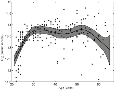
Figure1is a scatterplot of age versus log(income) for a sample ofn= 205 Canadian workers, all of whom were educated to grade 13. These data were used in Ullah (1985), and their source is a 1971 Canadian Census Public Use Tape.
3.1. Model and priors
The mean of log(income) as a function of age was modeled using thin-plate splines with K = 20 knots chosen so that the k-th knot is the sample quantile of age corresponding to probabilityk/(K+ 1). We used model (3) whereyi,xi denote the log income and age of the i-th worker. The following priors were used
β0, β1 ∼ N(0,106)
σ−2b , σ−2 ∼ Gamma 10−6,10−6 , (4) where the second parameter of the normal distribution is the variance. In many applications a normal prior distribution centered at zero with a standard error equal to 1000 is sufficiently noninformative. If there are reasons to suspect, either using alternative estimation methods or prior knowledge, that the true parameter is in another region of the space, then the prior should be adjusted accordingly. The parametrization of the Gamma(a, b) distribution is chosen so that its mean is a/b= 1 and its variance is a/b2 = 106. In Section8 we discuss several issues related to prior choice for nonparametric smoothing.
3.2. WinBUGS program for age–income data
We now describe theWinBUGS program that follows closely the description of the Bayesian nonparametric model in Equation (3) with the priors defined in (4). We provide the entire
20 30 40 50 60 11.5 12 12.5 13 13.5 14 14.5 15 Age (years)
Log (annual income)
Figure 1: Scatterplot of log(income) versus age for a sample of n= 205 Canadian workers with posterior median (solid) and 95% credible intervals for the mean regression function
program in AppendixA. While this program was designed for the age–income data, it can be used for other penalized spline regression models with minor adjustments. Many features of the program will be repeated in other examples and changes will be described, as needed. The likelihood part of the model (3) is specified inWinBUGSas follows
for (i in 1:n) {response[i]~dnorm(m[i],taueps) m[i]<-mfe[i]+mre110[i]+mre1120[i] mfe[i]<-beta[1]*X[i,1]+beta[2]*X[i,2] mre110[i] <-b[1]*Z[i,1]+b[2]*Z[i,2]+b[3]*Z[i,3]+b[4]*Z[i,4]+ b[5]*Z[i,5]+b[6]*Z[i,6]+b[7]*Z[i,7]+b[8]*Z[i,8]+ b[9]*Z[i,9]+b[10]*Z[i,10] mre1120[i]<-b[11]*Z[i,11]+b[12]*Z[i,12]+b[13]*Z[i,13]+b[14]*Z[i,14]+ b[15]*Z[i,15]+b[16]*Z[i,16]+b[17]*Z[i,17]+b[18]*Z[i,18]+ b[19]*Z[i,19]+b[20]*Z[i,20]}
The number of subjects, n, is a constant in the program. The first statement specifies that the i-th response (log income of the i-th worker) has a normal distribution with mean mi and precisionτ=σ−2 . The second statement provides the structure of the conditional mean function,mi =m(xi). Herebeta[]denotes the 2×1 dimensional vectorβ= (β0, β1), which is the vector of fixed effects parameters. Theith row of matrixX isXi = (1, xi). Similarly,b[] denotes the 20×1 dimensional vectorb= (b1, . . . , bk) of random coefficients. Both the matrix
X and Z = ZKΩ −1/2
K are design matrices obtained outside WinBUGS and are entered as data. In Section9 we discuss an auxiliaryRprogram that calculates these matrices and uses
theR2WinBUGSpackage to callWinBUGSfromR. Such programs would be especially useful
in a simulation study. The formulae formre110[]and mre1120[] could be shortened using the inner product function inprod. However, depending on the application, computation time can be 5 to 10 times longer wheninprod is used.
The distribution of the random coefficientsbis represented inWinBUGSas for (k in 1:num.knots){b[k]~dnorm(0,taub)}
This specifies that thebkare independent and normally distributed with mean 0 and precision τb =σb−2. Here num.knots is the number of knots (K = 20) and is introduced in WinBUGS as a constant. The prior distributions of model parameters described in Equation (4) are specified inWinBUGS as follows
for (l in 1:2){beta[l]~dnorm(0,1.0E-6)} taueps~dgamma(1.0E-6,1.0E-6)
taub~dgamma(1.0E-6,1.0E-6)
The prior normal distributions for the β parameters are expressed in terms of the precision parameter and the Gamma distributions are specified for the precision parameters τ =σ−2 and τb =σ−2b .
Note that the code is very short and intuitive presenting the model specification in rational steps. After writing the program one needs to load the data: the n-dimensional vector
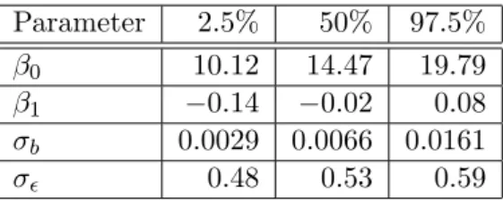
Parameter 2.5% 50% 97.5%
β0 10.12 14.47 19.79
β1 −0.14 −0.02 0.08
σb 0.0029 0.0066 0.0161
σ 0.48 0.53 0.59
Table 1: Posterior median and 95% credible interval for some parameters of model (3) for the Canadian age–income data
response (y) and the design matrices X[,] (X) and Z[,] (Z), the sample size n (n), the number of knotsnum.knots(K). At this stage the program needs to be compiled and initial values for all random variables have to be loaded.
3.3. Model inference
Convergence to the posterior distributions was assessed using several initial values of model parameters and visually inspecting several chains corresponding to the model parameters. Convergence was attained in less than 1,000 simulations, but we discarded the first 10,000 burn-in simulations. For inference we used 90,000 simulations. These simulations took ap-proximately 6 minutes on a PC (3.6GB RAM, 3.4GHz CPU).
Table 1 shows the posterior median and a 95% credible interval for some of the model pa-rameters. We also obtained the posterior distributions of the mean function of the response, mi = m(xi). Figure 1 displays the median, 2.5% and 97.5% quantiles of these posterior distributions for each value of the covariate xi. The greyed area corresponds to pointwise credible intervals for each m(xi) and is not a joint credible band for the mean function. An important advantage of Bayesian over the typical frequentist analysis is that in the Bayesian case the credible intervals take into account the variability of each parameter and do not use the “plug-in” method. Prediction intervals at an in-samplexvalue can be obtained very easily by monitoring random variables of the type
yi∗ =mi+∗i ,
with∗i being independent realizations of the distributionN(0, σ2). This can be implemented by adding the following lines to the WinBUGS code
for (i in 1:n)
{epsilonstar[i]~dnorm(0,taueps) ystar[i]<-m[i]+epsilonstar[i]}
4. The wage–union membership data
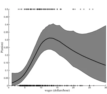
Figure 2 displays data on wages and union membership for 534 workers described inBerndt (1991). The data were taken from the Statlib website at Carnegie Mellon University http:
//lib.stat.cmu.edu/. This data set was analyzed in Ruppert et al. (2003) and standard
0 5 10 15 20 25 30 0 0.05 0.1 0.15 0.2 0.25 0.3 0.35 0.4 0.45 wages (dollars/hour) P(union)
Figure 2: Logistic spline fit to the union and wages scatterplot (solid) with 95% credible sets. Raw data are plotted as pluses, but with values of 1 for union replaced by 0.5 for graphical purposes. A worker making USD 44.50 per hour was used in the fitting but not shown to increase detail.
model the logit of the union membership probability as a penalized spline, which allows identification of features that are not captured by standard regression techniques. In this section we show how to implement a semiparametric Bernoulli regression inWinBUGS using low-rank thin-plate splines.
4.1. Generalized P-spline model
Denote byythe binary union membership variable, byxthe continuous wage variable and by p(x) the union membership probability for a worker with wage xin USD per hour. The logit of p(x) is modeled nonparametrically using a linear (p = 1) penalized spline with K = 20 knots. We used the following model
yi|xi ∼ Bernoulli{p(xi)} logit{p(xi)} = β0+β1xi+ PK k=1bkzik bk ∼ N(0, σb2) i ∼ N(0, σ2) , (5)
where zik is the (i, k)th entry of the design matrixZ =ZKΩ −1/2
K defined in Section2. The following prior distributions were used
β0, β1 ∼ N(0,106)
Parameter 2.5% 50% 97.5%
β0 −7.48 −4.15 −2.43
β1 −0.03 0.34 1.08
σb 0.045 0.100 0.229
Table 2: Posterior median and 95% credible interval for some parameters of the model presented in Equations (5) and (6)
4.2. WinBUGS program for wage–union data
While model (5) is very similar to model (3) the Bayesian analysis implementation in MAT-LAB,C or other software is significantly different. Typically, when the model is changed one needs to rewrite the entire code and make sure that all code bugs have been removed. This is a lengthy process that requires a high level of expertise in statistics and MCMC coding.
WinBUGScuts short this difficult process, thus making Bayesian analysis appealing to a larger audience.
In this case, changing the model from (3) to (5) requires only small changes in theWinBUGS
code. Specifically, the two lines specifying the conditional distribution of the response variable are replaced with
for (i in 1:n)
{response[i]~dbern(p[i])
logit(p[i])<-mfe[i]+mre110[i]+mre1120[i]}
while the rest of the code remains practically unchanged. Given this very simple change, we do not provide the rest of the code here, but we provide a commented version in the accompanying software file.
4.3. Model inference
Table 2 shows the posterior median and a 95% credible interval for some of the model pa-rameters. We also obtained the posterior distributions of pi = p(xi) and Figure 2 displays the median, 2.5% and 97.5% quantiles of these distributions. The greyed area corresponds to credible intervals for each p(xi) and is not a joint credible band. The credible intervals take into account the variability of each parameter. Convergence was attained in less than 1,000 simulations, but we discarded the first 10,000 burn-in simulations. For inference we used 90,000 simulations. These simulations took approximately 80 minutes on a PC (3.6GB RAM, 3.4GHz CPU).
5. The Sitka spruce data
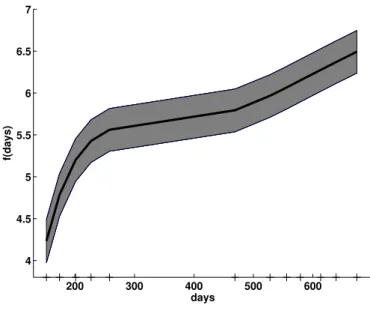
The mixed model representation of penalized splines allows simple extensions to additive mixed models. As an example we will use data on the growth of Sitka spruces displayed in Figure 1.3 in Diggle, Heagerty, Liang, and Zeger (2002). The data consist of growth mea-surements of 79 trees over two seasons: 54 trees were grown in an ozone-enriched atmosphere while the remaining 25 comprise the control group.
200 300 400 500 600 4 4.5 5 5.5 6 6.5 7 days f(days)
Figure 3: Thin-plate spline fit for the function f(·) for Sitka spruce data (solid) with 95% credible sets. Sampling days are plotted as pluses.
5.1. Additive mixed models
A useful mixed model for the Sitka data is
yij = Ui+αwi+f(xij) +ij
Ui ∼ N(0, σ2U) , (7)
whereyij, 1 ≤ i≤ 79, 1 ≤j ≤13, is the log size of spruce i at the time of measurement j taken on day xij. Also Ui are independent random intercepts for each tree, wi is the ozone exposure indicator andij are random errors. We modelf(·) using low-rank thin-plate splines
f(xij) = β0+β1xij+ PK k=1bkzijk bk ∼ N(0, σ2b) , (8)
where thexijobservations are stacked in one vector and (ij) corresponds to the{13∗(i−1) +j}th observation. Herezijk is the (13∗(i−1) +j, k)th entry of the design matrix Z=ZKΩ−1K /2 defined in Section 2. The random parameters bk are assumed independent normal with σb2 controling the shrinkage of the thin-plate spline function towards the first degree polynomial.
5.2. WinBUGS program for the Sitka spruce data
The WinBUGS program has essentially the same structure as the previous programs. The likelihood part of the program is
for (k in 1:n)
{log.size[k]~dnorm(mu[k],tauepsilon) mu[k]<-U[id.num[k]]+alpha*ozone[k]+m[k]
m[k]<-beta[1]*X[k,1]+beta[2]*X[k,2]+b[1]*Z[k,1]+b[2]*Z[k,2]+ b[3]*Z[k,3]}
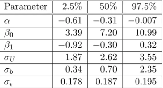
Parameter 2.5% 50% 97.5% α −0.61 −0.31 −0.007 β0 3.39 7.20 10.99 β1 −0.92 −0.30 0.32 σU 1.87 2.62 3.55 σb 0.34 0.70 2.35 σ 0.178 0.187 0.195
Table 3: Posterior median and 95% credible interval for some parameters of the model pre-sented in Equations (7) and (8)
The indexing structure is induced by stacking the vectors of observations corresponding to trees. For example thekth observation corresponds to the index (i, j) such thatk= 13∗(i−
1) +j. The first line of the program specifies that, conditional on its meanyij are independent with meanµij and precisionτ = 1/σ2. The second line of of code specifies the structure of the mean function as the sum between a random interceptUi, the ozone treatment effectαwi and a nonparametric mean functionf(·). The third line describes the mean function f(·) as a low-rank thin-plate spline.
Nested indexing is a powerful feature of WinBUGS and was used here to define the clusters corresponding to trees. To achieve this we defined a new vectorid.num[] which is the tree indicator. More precisely,id.num[k]=i if and only if thekth observation corresponds to tree i. In this way U[id.num[k]]isUi, the random intercept corresponding to treei, if and only ifkth observation corresponds to treei.
The distribution of random intercepts is specified as for (i in 1:M){U[i]~dnorm(0,tauU)}
where M = 79 is a constant in the program and tauU is the precision τU = 1/σU2 of the random intercept. The rest of the program is identical to the program for age and log income data and is omitted. A file containing the commented program and the corresponding R
programs is attached.
5.3. Model inference
Table 3 shows the posterior median and a 95% credible interval for some of the model pa-rameters. We also obtained the posterior distributions of f(xij) and Figure 3 displays the median, 2.5% and 97.5% quantiles of these distributions. The greyed area corresponds to credible intervals for eachf(xij)) and is not a joint credible band. Convergence was attained in less than 1,000 simulations, but we discarded the first 10,000 burn-in simulations. For inference we used 90,000 simulations. These simulations took approximately 5.5 minutes on a PC (3.6GB RAM, 3.4GHz CPU).
6. The coronary sinus potassium data
We consider the coronary sinus potassium concentration data measured on 36 dogs published inGrizzle and Allan(1969). The measurements on each dog were taken every 2 minutes from 1 to 13 minute (7 observations per dog). The 36 dogs come from 4 treatment groups.
Four smoothing spline analyses of these data were presented in Wang(1998). InCrainiceanu and Ruppert (2004b) is presented a hierarchical model of curves including a nonparametric overall mean, nonparametric treatment deviations from the overall curve, and nonparametric subject deviations from the treatment curves. In this section we show how to implement such a complex model in WinBUGS.
6.1. Longitudinal nonparametric ANOVA model
Denote byyij andtijthe potassium concentration and time for dogiat timej(in this example tij = 2j−1, but we keep the presentation more general). Consider the following model for potassium concentration
yij =f(tij) +fg(i)(tij) +fi(tij) +ij , (9)
where f(·) is the overall curve, fg(i)(·) are the deviations of the treatment group from the overall curve and fi(·) are the deviations of the subject curves from the group curves. Here g(i) represents the treatment group index corresponding to subjecti. All three functions are modeled as low-rank thin-plate splines as follows
f(t) = β0+β1t+ PK1 k=1bkztk fg(t) = γ0gI(g>1)+γ1gtI(g>1)+ PK2 k=1cgkz (g) tk fi(t) = δ0i+δ1it+PKk=13 dikztk(i) (10)
where I(g>1) is the indicator thatg >1, that is that the treatment group is g= 2, or 3 or 4. Hereztk is the (t, k)th entry of the design matrix for the thin-plate spline random coefficients,
Z = ZKΩ −1/2
K corresponding to the overall mean function f(·). Similarly, we defined z (g) tk and z(tki)as the (t, k)th entries of the design matrices for random coefficients corresponding to the group level fg(·), 1 ≤g ≤ 4, and subject level curves fi(·), 1 ≤i ≤36. The number of knots can be different for each curve and one can choose, for example, more knots to model the overall curve than each subject specific curve. However, in our example we used the same knots for each curve (K1 =K2 =K3 = 3).
The model also assumes that the b,c,dand δ parameters are mutually independent and bk ∼ N(0, σ2b), k= 1, . . . , K1 cgk ∼ N(0, σ2c), g= 1, . . . ,4, k = 1, . . . , K2 dik ∼ N(0, σ2d), i= 1, . . . , N, k= 1, . . . , K3 δ0i ∼ N(0, σ20), i= 1, . . . , N δ1i ∼ N(0, σ21), i= 1, . . . , N , (11)
where σ2b, σ2c and σd2 control the amount of shrinkage of the overall, group and individual curves respectively and σ02 andσ21 are the variance components of the subject random inter-cepts and slopes. We could also add other covariates that enter the model parametrically or
nonparametrically, consider different shrinkage parameters for each treatment group, etc. All these model transformations can be done very easily inWinBUGS.
To completely specify the Bayesian nonparametric model one needs to specify prior distribu-tions for all model parameters. The following priors were used
β0, β1, γ0g, γ1g ∼ N(0,106), g = 1, . . . ,4
σb−2, σ−2c , σ−2d , σ−2 , σ−20 , σ−21 ∼ Gamma 10−6,10−6 . (12)
6.2. WinBUGS program for the dog data
We provide the entireWinBUGS code for this model in Appendix B. Equation (10) is coded inWinBUGSas for (k in 1:n) {response[k]~dnorm(m[k],taueps) m[k]<-f[k]+fg[k]+fi[k] f[k]<-beta[1]*X[k,1]+beta[2]*X[k,2]+b[1]*Z[k,1]+ b[2]*Z[k,2]+b[3]*Z[k,3] fg[k]<-(gamma[group[k],1]*X[k,1]+gamma[group[k],2]*X[k,2]) *step(group[k]-1.5)+c[group[k],1]*Z[k,1]+ c[group[k],2]*Z[k,2]+c[group[k],3]*Z[k,3] fi[k]<-delta[dog[k],1]*X[k,1]+delta[dog[k],2]*X[k,2]+ d[dog[k],1]*Z[k,1]+d[dog[k],2]*Z[k,2]+d[dog[k],3]*Z[k,3]} The response is organized as a column vector obtained by stacking the information for each dog. Because there are 7 observations for each dog, the observation numberk can be written explicitly in terms of (i, j), that is k = 7(i−1) +j. The number of observations is n = 36×7 = 252.
We used twon×1 column vectors with entriesdog[k]and group[k], that store the dog and treatment group indexes corresponding to thek-th observation.
The first two lines of code in theforloop correspond to Equation (9), wherednormspecifies thatresponse[k]has a normal distribution with meanm[k]and precisiontaueps. The mean of the response is specified to be the sum off[k],fg[k] andfi[k], which are the variables for the overall mean, treatment group deviation from the mean and individual deviation from the group curves.
The following lines of code in thefor loop describe the structure of these curves in terms of splines. We keep the same notations from the previous sections. Because in this example we use the same knots and covariates the matricesXand Zdo not change for the three types of curves.
The definition of the overall curve f[k] follows exactly the same procedure with the one described in Section 3.2. The definition of fg[k] follows the same pattern but it involves two WinBUGS specific tricks. The first one is the use of the step function, described in Section 5.2. Here step(group[k]-1.5) is 1 if the index of the group corresponding to the k-th observation is larger than 1.5 and zero otherwise. This captures the structure of the fg(·) function in Equation (10) because the possible values of group[k] are 1, 2, 3 and 4. The second trick is the nested indexing used in the definition of theγ andcparameters using
thedogs vector described above. For example, theγ parameters are stored in a 4×2 matrix gamma[,]with theg-th linegamma[g,]corresponding to the parametersγ0g,γ1g of thefg(·) function. Note that if g is replaced bygroup[k]we obtain the parameters corresponding to the k-th observation. Similarly,c[,]stores the cgk parameters offg(·) and is a 4×3 matrix because there are 4 treatment groups and 3 knots. The definition of fi[k] curve uses the same ideas, with the only difference that the vectordog[k]is used instead ofgroup[k]. Here, delta[,] is a 36×2 matrix with the i-th line containing the δ0i and δ1i, the random slope and intercept corresponding to thei-th dog. Also, d[,]is a 36×3 matrix with the i-th line storing thedi1,di2 anddi3, the parameters of the truncated polynomial functions for thei-th dog.
TheWinBUGScoding of the distributions ofb,c,dandδfollows almost literally the definitions provided in Equation (11) for (k in 1:num.knots){b[k]~dnorm(0,taub)} for (k in 1:num.knots) {for (g in 1:ngroups){c[g,k]~dnorm(0,tauc)}} for (i in 1:ndogs) {for (k in 1:num.knots){d[i,k]~dnorm(0,taud)}} for (i in 1:ndogs) {for (j in 1:2){delta[i,j]~dnorm(0,taudelta[j])}}
For example, the parameters cj,k are assumed to be independent with distribution N(0, σc2) and theWinBUGScode is c[g,k]~dnorm(0,tauc). Herenum.knots,ngroupsandndogsare the number of knots of the spline, the number of treatment groups and the number of dogs respectively. These are constants and are entered as data in the program. Using the same notations as in Section3.2the normal prior distributions described in Equation (12) are coded as
for (l in 1:2){beta[l]~dnorm(0,1.0E-6)} for (l in 1:2)
{for (j in 1:ngroups){gamma[j,l]~dnorm(0,1.0E-6)}} and the prior gamma distributions on the precision parameters are coded as
taub~dgamma(1.0E-6,1.0E-6) tauc~dgamma(1.0E-6,1.0E-6) taud~dgamma(1.0E-6,1.0E-6) taueps~dgamma(1.0E-6,1.0E-6)
for (j in 1:2){taudelta[j]~dgamma(1.0E-6,1.0E-6)}
Here taub, tauc, taud and taueps are the precisions σb−2, σ−2c , σd−2 and σ−2 respectively. taudelta[1]and taudelta[2] are the precisionsσ0−2 and σ1−2 for the δ-parameters.
6.3. Model inference
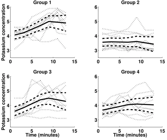
Figure4 shows the data for the 36 dogs corresponding to each treatment group together with the posterior mean and 90% credible interval for the treatment group mean functions. Recall
0 5 10 15 3 4 5 6 Group 1 Potassium concentration 0 5 10 15 3 4 5 6 Group 2 0 5 10 15 3 4 5 6 Group 3 Time (minutes) Potassium concentration 0 5 10 15 3 4 5 6 Group 4 Time (minutes)
Figure 4: Coronary sinus potassium concentrations for 36 dogs in four treatment groups with posterior median and 90% credible intervals of the group means. The dotted lines represent the individual dog data. The solid lines are the posterior medians of the group means. The dashed lines are the 5% and 95% quantiles of the posterior distributions of the group means. that the treatment group functions are the sums between the overall mean function and the functions for the treatment group deviations from the mean functions, that is
fgroup(t) =f(t) +fg(t)
This is achieved inWinBUGS by monitoring a new variablefgroup[]defined as for (k in 1:n){fgroup[k]<-f[k]+fg[k]}
For inference we used 90,000 simulations. These simulations took approximately 4.5 minutes on a PC (3.6GB RAM, 3.4GHz CPU).
7. Improving mixing
Mixing is the property of the Markov chain to move rapidly throughout the support of the posterior distribution of the parameters. Improving mixing is very important especially when computation speed is affected by the size of the data set or model complexity. In this section we present a few simple but effective techniques that help improve mixing.
Model parametrization can dramatically affect MCMC mixing even for simple parametric models. Therefore careful consideration should be given to the complex semiparametric mod-els, such as those considered in this paper. Probably the most important step for improving mixing in this framework is careful choice of the spline basis. While we have experimented with other spline bases, the low-rank thin-plate splines seem best suited for the MCMC sam-pling in WinBUGS. This is probably due to the reduced posterior correlation between the spline parameters. The truncated polynomial basis provides similar inferences about the mean function but mixing tends to be very poor with serious implications about the coverage probabilities of the pointwise confidence intervals.
In our experience with WinBUGS, centering and standardizing the covariates also improve, sometimes dramatically, mixing properties of simulated chains.
Another, less known technique is hierarchical centering (Gelfand, Sahu, and Carlin 1995b,a). Many statistical models contain random effects that are ordered in a natural hierarchy (e.g. observation/site/region). The hierarchical centering of random effects generally has a positive effect on simulation mixing and we recommend it whenever the model contains a natural hierarchy. Bayesian smoothing models presented in this paper also contain the exchangeable random effects, b, which are not part of an hierarchy and they cannot be “hierarchically centered”.
In Crainiceanu, Ruppert, Stedinger, and Behr (2002) it is shown that even for a simple Poisson-Log Normal model the amount of information has a strong impact on the mixing properties of parameters. A practical recommendation in these cases is to improve mixing, as much as possible, for a subset of parameters of interest. These model specification refinements pay off especially in slowWinBUGS simulations.
8. Prior specification
Any smoother depends heavily on the choice of smoothing parameter, and for P-splines in a mixed model framework, the smoothing parameter is the ratio of two variance components Ruppertet al.(2003). The smoothness of the fit depends on how these variances are estimated. For example, in Crainiceanu and Ruppert (2004a) it is shown that, in finite samples, the (RE)ML estimator of the smoothing parameter is biased towards oversmoothing.
In Bayesian mixed models, the estimates of the variance components are known to be sensitive to the prior specification, e.g., see Gelman (2004). To study the effect of this sensitivity upon Bayesian P-splines, consider model (3) with one smoothing parameter and homoscedastic er-rors. In terms of the precision parametersτb = 1/σ2b andτ = 1/σ2, the smoothing parameter is λ=τ/τb=σb2/σ2 and a small (large) λcorresponds to oversmoothing (undersmoothing). It is standard to assume that the fixed effects parameters, βi, are apriori independent, with prior distributions either [βi]∝1 orβi ∝N(0, σβ2), whereσβ2 is very large. In our applications we used σβ2 = 106, which we recommend if x and y have been standardized or at least have standard deviations with order of magnitude one.
As just mentioned, the priors for the precisionsτb andτ are crucial. We now show how criti-cally the choice ofτb may depend upon the scaling of the variables. If [τb]∼Gamma(Ab, Bb) and, independently of τb, [τ] ∼ Gamma(A, B) where Gamma(A, B) has mean A/B and
varianceA/B2, then [τb|Y,β,b, τ]∼Gamma Ab+ Km 2 , Bb+ ||b||2 2 (13) and [τ|Y,β,b, τ]∝Gamma A+ n 2, B+ ||Y −Xβ−Zb||2 2 . Also, E(τb|Y,β,b, τ) = Ab+Km/2 Bb+||b||2/2 , Var(τb|Y,β,b, τ) = Ab+Km/2 (Bb+||b||2/2)2 , and similarly forτ.
The prior does not influence the posterior distribution of τ when both Ab and Bb are small compared to Km/2 and ||b||2/2 respectively. Since the number of knots is Km ≥ 1 and in most problems considered Km ≥ 5, it is safe to choose Ab ≤ 0.01. When Bb << ||b||2/2 the posterior distribution is practically unaffected by the prior assumptions. When Bb in-creases compared to||b||2/2, the conditional distribution is increasingly affected by the prior assumptions. E(τb|Y,β,b, τ) is decreasing inBb so largeBb compared to||b||2/2 correspond to undersmoothing. Since the posterior variance ofτb is also decreasing inBb a poor choice of Bb will likely result in underestimating the variability of the smoothing parameterλ=τ/τb causing too narrow confidence intervals for m. The conditionBb <<||b||2/2 shows that the “noninformativeness” of the gamma prior depends essentially on the scale of the problem, because the size of||b||2/2 depends upon the scaling of thex andy variables. Ify is rescaled toayy and x toaxx, then the regression function becomes aym(axx) whose p-th derivative isayapxm(p)(axx) so that||b||2/2 is rescaled by the factora2ya
2p
x . Thus, ||b||2/2 is particularly sensitive to the scaling ofx.
A similar discussion holds true forτ but now largeB corresponds to oversmoothing and τ does not depend on the scaling ofx. In applications it is less likely that B is comparable in size to||Y −Xβ−Zb||2, because the latter is an estimator of nσ2
. If ˆσ2 is an estimator of σ2 a good rule of thumb is to use values of B smaller than nσˆ2/100. This rule should work well when ˆσ2 does not have an extremely large variance.
Alternative to gamma priors are discussed by, for example, inGelman(2004);Natarajan and Kass (2000). These have the advantage of requiring less care in the choice of the hyperpa-rameters. However, we find that with reasonable care, the conjugate gamma priors can be used in practice. Nonetheless, exploration of other prior families for P-splines would be well worthwhile, though beyond the scope of this paper.
9. Interface with and processing in
R
WinBUGS 1.4 provides a Graphical User Interface (GUI) that is user friendly and provides important information including the chain histories that can be used to asses mixing. However, theWinBUGS script language is relatively limited and is hard to use for effective simulation studies involving repeated calls forWinBUGS.
R2WinBUGSSturtzet al.(2005) is anRpackage that callsWinBUGS1.4 and exports results
functions for each model described in this paper are attached to this paper. We present here important parts of theRcode, while commented Rprograms are attached to this paper. The Rprogram starts with
data.file.name="smoothing.norm.txt" program.file.name="scatter.txt" inits.b=rep(0,20)
inits<-function(){list(beta=c(0,0),b=inits.b,taub=0.01,taueps=0.01)} parameters<-list("lambda","sigmab","sigmaeps","beta","b","ystar")
The first two code lines define the file names for data and WinBUGS program respectively. The third and fourth lines define the initial values to be used in theWinBUGS program and the fifth line indicates the name of the parameters to be monitored in the MCMC sampling. These parameters must correspond to parameters in theWinBUGSprogram. TheRprogram continues with data<-read.table(file=data.file.name,header=TRUE) attach(data) n<-length(covariate) X<-cbind(rep(1,n),covariate) knots<-quantile(unique(covariate), seq(0,1,length=(num.knots+2))[-c(1,(num.knots+2))])
The first and second lines read and attach the data, the third line defines the sample size, and the fourth line defines the X matrix of fixed effects for the thin-plate spline. The last assignment defines thenum.knots number of knots at the sample quantiles of the covariate. An important step in using thin-plate splines is to define theZK,ΩK and the design matrix of random coefficients Z=ZKΩ
−1/2
K . The following lines of code achieve this Z_K<-(abs(outer(covariate,knots,"-")))^3 OMEGA_all<-(abs(outer(knots,knots,"-")))^3 svd.OMEGA_all<-svd(OMEGA_all) sqrt.OMEGA_all<-t(svd.OMEGA_all$v %*% (t(svd.OMEGA_all$u)*sqrt(svd.OMEGA_all$d))) Z<-t(solve(sqrt.OMEGA_all,t(Z_K)))
At this stage data is defined, WinBUGS is called from R and the output of the program is loaded intoRfor further processing. The main function for doing this is bugs()implemented in the R2WinBUGSpackage.
data<-list("response","X","Z","n","num.knots")
Bayes.fit<- bugs(data, inits, parameters, model.file = program.file.name, n.chains = 1, n.iter = n.iter, n.burnin = n.burnin,
n.thin = n.thin,debug = FALSE, DIC = FALSE, digits = 5,
codaPkg = FALSE,bugs.directory = "c:/Program Files/WinBUGS14/") attach.all(Bayes.fit)
10. Pros and cons
An advantage of WinBUGS is the simple programming that translates almost literally the Bayesian model into code. This saves time by avoiding the usually lengthy implementations of the MCMC simulation algorithms. For example, total programming time for one model is approximately 1 to 2 hours. Programs designed by experts for specific problems can be more refined by taking into account properties of the model and using a combination of art and experience to improve mixing and computation time. However, when we compare aWinBUGS
with an expert program in terms of computation speed, programming time needs to be taken into account.
WinBUGSallows simple model changes to be reflected in simple code changes, which encour-ages the practitioner or the expert to investigate a much wider spectrum of models. Expert programs are usually restrictive in this sense.
Our recommendation is to start withWinBUGS, implement the model for the specific data set. If it runs in a reasonable time and has good mixing properties, then continue withWinBUGS. Otherwise consider designing an expert program. Even if one decides to use the expert program we still recommend using WinBUGSas a method of checking results. Programming errors and debugging time are also dramatically reduced inWinBUGS.
References
Berndt E (1991). The Practice of Econometrics: Classical and Contemporary. Addison– Wesley, Reading MA, USA.
Berry S, Carroll RJ, Ruppert D (2002). “Bayesian Smoothing and Regression Splines for Measurement Error Problems.” Journal of the American Statistical Association, 97, 160– 169.
Brumback B, Ruppert D, Wand MP (1999). “Comment on Variable Selection and Func-tion EstimaFunc-tion in Additive Nonparametric Regression Using Data–based Prior by Shively, Kohn, and Wood.”Journal of the American Statistical Association,94, 794–797.
Crainiceanu CM, Ruppert D (2004a). “Likelihood Ratio Tests in Linear Mixed Models with One Variance Component.”Journal of the Royal Statistical Society B,66, 165–185. Crainiceanu CM, Ruppert D (2004b). “Restricted Likelihood Ratio Tests in Nonparametric
Longitudinal Models.”Statistica Sinica,14.
Crainiceanu CM, Ruppert D, Stedinger JR, Behr CT (2002). “Improving MCMC Mixing for a GLMM Describing Pathogen Concentrations in Water Supplies.” In C Gatsonis, RE Kass, A Carriquiry, A Gelman, D Higdon, DK Pauler, I Verdinelli (eds.), “Case Studies in Bayesian Statistics,” volume 6. Springer-Verlag, New York.
Diggle P, Heagerty P, Liang K, Zeger S (2002). Analysis of Longitudinal Data. Oxford University Press, New York, USA.
Eilers P, Marx B (1996). “Flexible Smoothing with B-splines and Penalties.” Statistical Science,11(2), 89–121.
Eubank R (1988). Spline Smoothing and Nonparametric Regression. Marcel Dekker, New York, USA.
Fan J, Gijbels I (1996). Local Polynomial Modeling and its Applications. Chapman and Hall, London, UK.
Friedman J (1991). “Multivariate Adaptive Regression Splines (with Discussion).”The Annals of Statistics,19, 1–141.
Gelfand A, Sahu S, Carlin B (1995a). “Efficient Parameterizations for Normal Linear Mixed Model.” In AD JM Bernardo J Berger, A Smith (eds.), “Bayesian Statistics,” volume 5. Oxford University Press, Oxford, UK.
Gelfand A, Sahu S, Carlin B (1995b). “Efficient Parameterizations for Normal Linear Mixed Models.”Biometrika,3, 479–488.
Gelman A (2004). “Prior Distributions for Variance Parameters in Hierarchical Models.” manuscript.
Green P, Silverman B (1994). Nonparametric Regression and Generalized Linear Models. Chapman and Hall, London, UK.
Grizzle J, Allan D (1969). “Analysis of Dose and Dose Response Curves.” Biometrics, 25, 357–381.
Hansen M, Kooperberg C (2002). “Spline Adaptation in Extended Linear Models (with Discussion).”Statistical Science,17, 2–51.
Hastie T, Tibshirani R (1990). Generalized Additive Models. Chapman and Hall, London, UK.
Insightful Corp (2003). S-PLUS 6.2. Seattle, WA.
Natarajan R, Kass R (2000). “Reference Bayesian Methods for Generalized Linear Mixed Models.”Journal of the American Statistical Association,95, 227–237.
Ngo L, Wand M (2004). “Smoothing with Mixed Model Software.” Journal of Statistical Software,9(1). URL http://www.jstatsoft.org/v09/i01/.
Ogden R (1996). Essential Wavelets for Statistical Applications and Data Analysis. Birkhauser, Boston, USA.
RDevelopment Core Team (2005).R: A Language and Environment for Statistical Computing.
RFoundation for Statistical Computing, Vienna, Austria. ISBN 3-900051-07-0, URLhttp:
//www.R-project.org/.
Ruppert D (2002). “Selecting the Number of Knots for Penalized Splines.”Journal of Com-putational and Graphical Statistics,11, 735–757.
Ruppert D, Wand M, Carroll R (2003). Semiparametric Regression. Cambridge University Press, Cambridge, UK.
Spiegelhalter D, Thomas A, Best N (2003). WinBUGS Version 1.4 User Manual. Medical Research Council Biostatistics Unit, Cambridge, UK.
Sturtz S, Ligges U, Gelman A (2005). “R2WinBUGS: A Package for RunningWinBUGSfrom
R.”Journal of Statistical Software,12(3). URL http://www.jstatsoft.org/v12/i03/. Tarter M, Lock M (1993).Model–free Curve Estimation. Chapman and Hall, New York, USA. Ullah A (1985). “Specification Analysis of Econometric Models.” Journal of Quantitative
Economics,2, 187–209.
Wahba G (1990). Spline Models for Observational Data. Society for Industrial and Applied Mathematics, Philadelphia PA, USA.
Wand M (2003). “Smoothing and Mixed Models.”Computational Statistics,18, 223–249. Wand M, Jones M (1995). Kernel Smoothing. Chapman and Hall, London, UK.
Wang Y (1998). “Mixed Effects Smoothing Spline Analysis of Variance.” Journal of Royal Statistical Society B,60, 159–174.
A.
WinBUGS
code for the age–income example
Model
This is the complete code for scatterplot smoothing used in the age–income example.
model{ #Begin model
#This model can be used for any simple scatterplot smoothing. It #can be easily modified to accommodate other covariates and/or #random effects
#Likelihood of the model for (i in 1:n) {response[i]~dnorm(m[i],taueps) m[i]<-mfe[i]+mre110[i]+mre1120[i] mfe[i]<-beta[1]*X[i,1]+beta[2]*X[i,2] mre110[i]<-b[1]*Z[i,1]+b[2]*Z[i,2]+b[3]*Z[i,3]+b[4]*Z[i,4]+ b[5]*Z[i,5]+b[6]*Z[i,6]+b[7]*Z[i,7]+b[8]*Z[i,8]+ b[9]*Z[i,9]+b[10]*Z[i,10] mre1120[i]<-b[11]*Z[i,11]+b[12]*Z[i,12]+b[13]*Z[i,13]+b[14]*Z[i,14]+ b[15]*Z[i,15]+b[16]*Z[i,16]+b[17]*Z[i,17]+b[18]*Z[i,18]+ b[19]*Z[i,19]+b[20]*Z[i,20]}
#Prior distributions of the random effects parameters for (k in 1:num.knots){b[k]~dnorm(0,taub)}
#Prior distribution of the fixed effects parameters for (l in 1:2){beta[l]~dnorm(0,1.0E-6)}
#Prior distributions of the precision parameters
taueps~dgamma(1.0E-6,1.0E-6); taub~dgamma(1.0E-6,1.0E-6)
#Deterministic transformations. Obtain the standard deviations and #the smoothing parameter
sigmaeps<-1/sqrt(taueps);sigmab<-1/sqrt(taub) lambda<-pow(sigmab,2)/pow(sigmaeps,2)
#Predicting new observations for (i in 1:n)
{epsilonstar[i]~dnorm(0,taueps) ystar[i]<-m[i]+epsilonstar[i]}
Data
Data consists of the response variable (response[]) design matrix for fixed effects (X[,]) design matrix of random effects (Z[,]) sample size (n), and number of knots (num.knots).
Initial values
Initial values are provided for the fixed effectsβ (beta[]) random coefficientsb(b[]) precision τb (taub) and precisionτ (taueps). All other initial values are generated by WinBUGSfrom their prior distributions.
Both data and initial values are specified and processed in R and then used in WinBUGS
through the bugs() function implemented in the R2WinBUGS package as described in Sec-tion 9.
B.
WinBUGS
code for coronary sinus potassium example
Model
This is the complete code for the Bayesian semiparametric model for coronary sinus potassium example presented in Section 6.
model{ #Begin model
#This model was designed for the coronary sinus potassium model #described in this paper. However, the basic coding ideas can be #applied more generally to longitudinal models that involve a #hierarchy of parametric and/or nonparametric curves
#Likelihood of the model for (k in 1:n) {response[k]~dnorm(m[k],taueps) m[k]<-f[k]+fg[k]+fi[k] f[k]<-beta[1]*X[k,1]+beta[2]*X[k,2]+b[1]*Z[k,1]+ b[2]*Z[k,2]+b[3]*Z[k,3] fg[k]<-(gamma[group[k],1]*X[k,1]+gamma[group[k],2]*X[k,2]) *step(group[k]-1.5)+c[group[k],1]*Z[k,1]+ c[group[k],2]*Z[k,2]+c[group[k],3]*Z[k,3] fi[k]<-delta[dog[k],1]*X[k,1]+delta[dog[k],2]*X[k,2]+ d[dog[k],1]*Z[k,1]+d[dog[k],2]*Z[k,2]+d[dog[k],3]*Z[k,3]} #Prior for the random parameters of the overall curve
for (k in 1:num.knots){b[k]~dnorm(0,taub)}
#Prior for the random parameters for the curves describing group #deviations from the overall curve
for (k in 1:num.knots)
#Prior for the random parameters for the individual deviations #from the group curve
for (i in 1:ndogs)
{for (k in 1:num.knots){d[i,k]~dnorm(0,taud)}} #Prior for monomial parameters of the overall curve
for (l in 1:2){beta[l]~dnorm(0,1.0E-6)}
#Prior for monomial parameters of curves describing the group #deviations from the overall curve
for (l in 1:2)
{for (j in 1:ngroups){gamma[j,l]~dnorm(0,1.0E-6)}}
#Prior for monomial parameters of curves describing the individual #deviations from the group curve
for (i in 1:ndogs)
{for (j in 1:2){delta[i,j]~dnorm(0,taudelta[j])}} #Priors of precision parameters
taub~dgamma(1.0E-6,1.0E-6) tauc~dgamma(1.0E-6,1.0E-6) taud~dgamma(1.0E-6,1.0E-6) taueps~dgamma(1.0E-6,1.0E-6)
for (j in 1:2){taudelta[j]~dgamma(1.0E-6,1.0E-6)} #Define the group curves
for (i in 1:n){fgroup[i]<-f[i]+fg[i]}
} #End model
Data
Data consists of the response variable (response[]) design matrix for fixed effects (X[,]) and design matrix of random effects (Z[,]), sample size (n), number of knots (num.knots), number of subjects (nsubjects), number of groups (ngroups), subject indicator vector (dog), and group vector indicator (group).
Initial values
Initial values are provided for the fixed effects for all curves β (beta[]), γ (gamma[,]), δ (delta[,]), random coefficients for all curvesb(b[]),c(c[,]),d(d[,]), precisionsτb(taub), τc (tauc),τd (taud) and precision τ (taueps).
Both data and initial values are specified and processed in Rand then used in WinBUGS
through the bugs() function implemented in the R2WinBUGS package as described in Sec-tion 9.
Affiliation:
Ciprian Crainiceanu
Department of Biostatistics Johns Hopkins University 615 N. Wolfe St. E3636
Baltimore, MD 21205, United States of America E-mail: [email protected]
URL:http://www.biostat.jhsph.edu/~ccrainic/
David Ruppert
School of Operational Research and Industrial Engineering Cornell University
Rhodes Hall, NY 14853, United States of America E-mail: [email protected]
URL:http://www.orie.cornell.edu/~davidr/
M.P. Wand
Department of Statistics School of Mathematics
University of New South Wales Sydney 2052, Australia
E-mail: [email protected]
URL:http://www.maths.unsw.edu.au/~wand/