Calibration of the Highway Safety Manual and development of new safety performance functions for rural multilane highways in Kansas

(1)

CALIBRATION OF THE HIGHWAY SAFETY MANUAL AND DEVELOPMENT OF NEW SAFETY PERFORMANCE FUNCTIONS FOR RURAL MULTILANE HIGHWAYS IN

KANSAS

by

SYEDA RUBAIYAT AZIZ

BS, Bangladesh University of Engineering and Technology, 2009 MS, Kansas State University, 2013

AN ABSTRACT OF A DISSERTATION

submitted in partial fulfillment of the requirements for the degree

DOCTOR OF PHILOSOPHY

Department of Civil Engineering College of Engineering

KANSAS STATE UNIVERSITY Manhattan, Kansas

(2)

Abstract

Rural roads account for 90.3% of the 140,476 total centerline miles of roadways in Kansas. In recent years, rural fatal crashes have accounted for about 66% of all fatal crashes. The Highway Safety Manual (HSM) provides models and methodologies for analyzing the safety of various types of highways. Predictive methods in the HSM were developed based on national trends and data from few states throughout the United States. However, these methodologies are of limited use if they are not calibrated for individual jurisdictions or local conditions.

The objective of this study was to analyze the HSM calibration procedures for rural multilane segments and intersections in Kansas. The HSM categorizes rural multilane segments as four-lane divided (4D) and four-lane undivided (4U) segments and rural multilane intersections as three-legged intersections with minor-road stop control (3ST), four-legged intersections with minor-road stop control (4ST), and four-leg signalized intersections (4SG). The number of predicted crashes at each segment was obtained according to the HSM calibration process. Results from calibration of rural segments indicated that the HSM overpredicts fatal and injury crashes by 50% and 65% and underpredicts total crashes by 48% and 64% on rural 4D and 4U segments, respectively. The HSM-given safety performance function (SPF) regression coefficients were then modified to capture variation in crash prediction. The adjusted models for 4D and 4U multilane segments indicated significant improvement in crash prediction for rural Kansas.

Furthermore, Kansas-specific safety performance functions (SPF)s were developed following the HSM recommendations. In order to develop Kansas-specific SPF, Negative Binomial regression was applied to obtain the most suitable model. Several additional variables were considered and tested in the new SPFs, followed by model validation on various sets of locations. The Kansas-specific SPFs are capable of more accurately predicting total and fatal and injury crashes on multilane segments compared to the HSM and the modified HSM models.

In addition to multilane segments, rural intersections on multilane highways were also calibrated according to the HSM methodology. Using crash modification factors for corresponding variables, SPFs were adjusted to obtain final predicted crash frequency at intersections. Obtained calibration factors indicated that the HSM is capable of predicting crashes at intersections at satisfactory level. Findings of this study can be used for improving safety of rural multilane highways.

(3)

CALIBRATION OF THE HIGHWAY SAFETY MANUAL AND DEVELOPMENT OF NEW SAFETY PERFORMANCE FUNCTIONS FOR RURAL MULTILANE HIGHWAYS IN

KANSAS

by

SYEDA RUBAIYAT AZIZ

BS, Bangladesh University of Engineering and Technology, 2009 MS, Kansas State University, 2013

A DISSERTATION

submitted in partial fulfillment of the requirements for the degree

DOCTOR OF PHILOSOPHY

Department of Civil Engineering College of Engineering

KANSAS STATE UNIVERSITY Manhattan, Kansas

2016

Approved by: Major Professor Sunanda Dissanayake

(4)

Abstract

Rural roads account for 90.3% of the 140,476 total centerline miles of roadways in Kansas. In recent years, rural fatal crashes have accounted for about 66% of all fatal crashes. The Highway Safety Manual (HSM) provides models and methodologies for analyzing the safety of various types of highways. Predictive methods in the HSM were developed based on national trends and data from few states throughout the United States. However, these methodologies are of limited use if they are not calibrated for individual jurisdictions or local conditions.

The objective of this study was to analyze the HSM calibration procedures for rural multilane segments and intersections in Kansas. The HSM categorizes rural multilane segments as four-lane divided (4D) and four-lane undivided (4U) segments and rural multilane intersections as three-legged intersections with minor-road stop control (3ST), four-legged intersections with minor-road stop control (4ST), and four-leg signalized intersections (4SG). The number of predicted crashes at each segment was obtained according to the HSM calibration process. Results from calibration of rural segments indicated that the HSM overpredicts fatal and injury crashes by 50% and 65% and underpredicts total crashes by 48% and 64% on rural 4D and 4U segments, respectively. The HSM-given safety performance function (SPF) regression coefficients were then modified to capture variation in crash prediction. The adjusted models for 4D and 4U multilane segments indicated significant improvement in crash prediction for rural Kansas.

Furthermore, Kansas-specific safety performance functions (SPF)s were developed following the HSM recommendations. In order to develop Kansas-specific SPF, Negative Binomial regression was applied to obtain the most suitable model. Several additional variables were considered and tested in the new SPFs, followed by model validation on various sets of locations. The Kansas-specific SPFs are capable of more accurately predicting total and fatal and injury crashes on multilane segments compared to the HSM and the modified HSM models.

In addition to multilane segments, rural intersections on multilane highways were also calibrated according to the HSM methodology. Using crash modification factors for corresponding variables, SPFs were adjusted to obtain final predicted crash frequency at intersections. Obtained calibration factors indicated that the HSM is capable of predicting crashes at intersections at satisfactory level. Findings of this study can be used for improving safety of rural multilane highways.

(5)

List of Figures

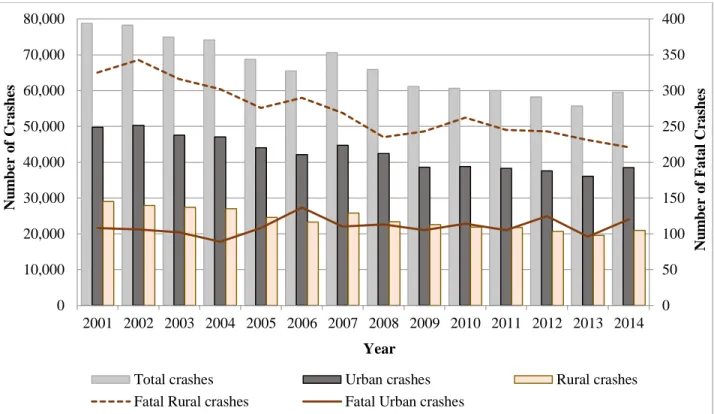
Figure 1.1 Yearly distribution of crashes in Kansas ...2

Figure 3.1 Using Google Map to obtain presence of lighting ... 24

Figure 3.2 Rural 4D segments and crash location map ... 26

Figure 3.3 Rural 4U segments and crash location map ... 27

Figure 3.4 4ST intersection with stop control at minor approach ... 42

Figure 3.5 3ST intersection with stop control at minor approach ... 42

Figure 3.6 Use of KDOT videologs ... 43

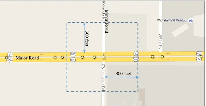
Figure 3.7 Intersection-box demonstration... 44

Figure 4.1 Distribution of crash frequency on 4D segments ... 51

Figure 4.2 Distribution of crash frequency on 4U segments ... 52

Figure 4.3 Distribution of crash frequency on 4ST intersections ... 64

Figure 4.4 Distribution of crash frequency on 3ST intersections ... 64

Figure 5.1 Total crashes: model 1 validation plot ... 90

Figure 5.5 Total crashes: model 1 validation plot (without outliers) ... 94

Figure 5.9 Fatal and injury crashes: model 1 validation plot ... 97

Figure 5.13 Fatal and injury crashes: model 1 validation plot (without outliers) ... 99

(9)

List of Tables

Table 3.1 Data sources for rural four-lane segments ... 25

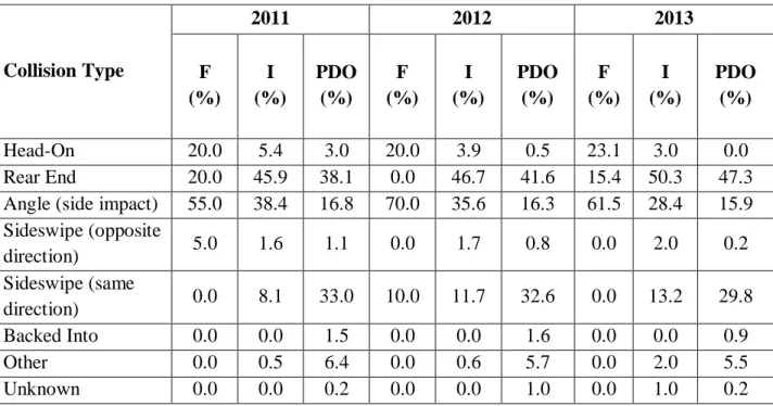
Table 4.1 Percentage of crashes by collision type for Kansas rural four-lane highways ... 47

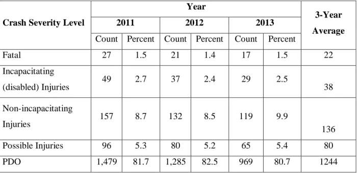
Table 4.2 Crash severity level on four-lane highways ... 48

Table 4.3 Crashes by collision type and severity level for four-lane roadways ... 49

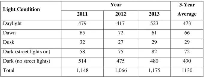
Table 4.4 Crash distribution by light condition ... 50

Table 4.5 Proportion of nighttime crashes for rural 4D and 4U highways in Kansas ... 50

Table 4.6 Descriptive statistics for rural four-lane segments ... 54

Table 4.7 4D segments sample worksheet ... 56

Table 4.8 Four-lane divided segments calibration factor calculation ... 57

Table 4.9 Four-lane undivided segments sample worksheet ... 58

Table 4.10 4U segments sample worksheet ... 59

Table 4.11 Comparison of regression coefficients ... 62

Table 4.12 New calibration factors with the modified SPF ... 63

Table 4.13 Descriptive statistics for rural multilane intersections ... 66

Table 4.14 4ST intersection sample worksheet ... 68

Table 4.15 Calculation of calibration factors for 4ST intersections ... 69

Table 4.16 3ST intersection sample worksheet ... 71

Table 4.17 Calculation of calibration factors for 3ST intersections ... 72

Table 5.1 Variables in new SPF development ... 76

Table 5.2 Curve classifications ... 77

Table 5.3 Vertical grade classifications ... 78

Table 5.4 Roadside hazard rating criterion... 79

Table 5.5 Descriptive statistics of variables ... 80

Table 5.6 Correlation analysis of variables ... 82

Table 5.7 Parameter estimates of model 1 for predicting total crashes ... 83

(10)

Table 5.12 Parameter estimates of model 2 for predicting fatal and injury crashes ... 86

Table 5.15 Goodness-of-fit comparison for total crashes model ... 89

Table 5.16 Goodness-of-fit comparison of fatal and injury crash models ... 96

Table 5.17 Comparison of model statistics ... 101

Table A.1 List of locations for 4D segment calibration ... 110

Table A.2 List of locations for 4U segment calibration ... 114

Table A.3 List of locations for 4ST intersections calibration ... 115

(11)

Acknowledgements

First, I would like to pay my utmost respect to Almighty Allah for granting me this wonderful opportunity to work and to live.

I hereby acknowledge my sincere appreciation and due gratitude to my major professor Dr. Sunanda Dissanayake for academic guidance, mentorship, and continuous support throughout my graduate studies. I am thankful to Dr. Robert Stokes, Dr. Eric Fitzsimmons, Dr. Margaret Rys, and Dr. John Leatherman for serving as my doctoral committee members.

I sincerely appreciate the Kansas Department of Transportation (KDOT) for funding this research. I gratefully thank Ms. Elsit Mandal, Mr. Rex McCommon, and Mr. Leif Holliday for their constant support with providing data to complete this research. I also appreciate the assistance that Austin Juaneman provided for intersection data collection.

Finally, I wish to express my sincere respect and gratitude to my parents, Dr. Syed Azizul Haque and Dr. Nilufar Begum for their encouragement, blessings, and love that helped me to be what I am today. I would like to especially thank my husband Dr. S M Shafiul Alam for his patience, support, and appreciation.

(12)

Dedication

This dissertation is dedicated to my late paternal grandfather Prof. Syed Mazharul Haq and late maternal grandfather Prof. Dr. Mufizur Rahman.

(13)

Chapter 1 - Introduction

1.1 Background

According to a study published in 2016, motor vehicle crashes were one of the top ten causes of death in the United States in 2013. Relative to 2011, fatal highway crashes increased by 1.7% to 29,989 in 2014, equivalent to an average of 90 daily fatalities (NHTSA, 2015). Despite the decline in fatalities, 32,675 deaths occurred as a result of roadway crashes in the United States in 2014, down from 32,894 in 2013 (NHTSA, 2015).

Rural roads account for 90.3% of the 140,476 total miles of roadway in Kansas (KDOT (a), 2015), and in 2014, rural travel accounted for 48.5% of all vehicle miles (60% for state highways) (KDOT (b), 2015). Figure 1.1 shows the distribution of rural, urban, fatal rural, fatal urban, and total crashes over a 14-year period. In general, Kansas has a low population density and a majority of the roadways are in rural areas. As shown in Figure 1.1, 35% of total crashes occurred on rural roads, while fatal crashes on rural roads accounted for over 66% of the number of total fatal crashes in Kansas during 2014 (KDOT, 2015). Not only in 2014, every year the number of fatal crashes in rural highways always been considerably higher than the fatal crashes on urban highways in Kansas. The time required to respond and transport crash victims potentially determines if the crash is classified as injury or fatal. In rural areas, transportation of severely injured crash victims to hospitals requires 60–120 minutes (NHTSA, 2009). These numbers are a matter of concern for highway safety professionals because they comprise a major proportion of high-level injury crashes in rural areas.

(14)

Figure 1.1 Yearly distribution of crashes in Kansas

1.2 Highway Safety Manual

The Highway Safety Manual (HSM) by the American Association of State Highway and Transport Officials (AASHTO) is the culmination of decades of safety research and practices

(AASHTO, 2010). The HSM provides models and methodologies for analyzing various types of highways based on safety. The first version, published in 2010, was updated in 2014 with new chapters on predictive methods for freeways and ramps. Procedures to calibrate predictive models are currently available in Part C – Appendix A of the HSM (AASHTO, 2010). Crash predictive methods in the HSM allow planners, designers, and reviewers to comprehensively assess expected safety performance of highway design via methodologies endorsed by the Federal Highway Administration

(FHWA). Predictive methods in the HSM were developed based on national trends and statistics

from sample states throughout the United States. However, these methodologies are of limited use

0 50 100 150 200 250 300 350 400 0 10,000 20,000 30,000 40,000 50,000 60,000 70,000 80,000 2001 2002 2003 2004 2005 2006 2007 2008 2009 2010 2011 2012 2013 2014 N u m b e r o f F atal C r as h e s N u m b e r o f C r as h e s Year

Total crashes Urban crashes Rural crashes

(15)

if they are not calibrated for individual jurisdictions or local conditions. Calibration ensures the most realistic and reliable crash estimates.

1.3 Problem Statement

Safety conditions of highways change over time; therefore, agencies should only use the HSM models that have been calibrated. Uncalibrated models compromise safety estimates, produce unrealistic results, and undermine accountability of highway safety. Even agencies that use their own data to develop SPFs should consider calibrating the models every two to three years in order for results to be comparable to estimates obtained from an agency’s records.

An acceptable method to predict crashes for rural multilane highway segments and intersections in Kansas must be developed. Currently, the Kansas Department of Transportation (KDOT) can apply the rural two-lane model given in HSM, because a previous study calibrated such facilities (Lubliner, 2012). KDOT has occasionally requested analysis of a multilane facility, but it cannot be completed without calibration. An effective equation that predicts the number of crashes along a highway and identifies potential high crash locations would enable design engineers to design safer roads while minimizing the cost if, for example, 8-ft. shoulders were determined to be as beneficial as 10-ft. shoulders.

Although calibration procedures are available in the HSM Appendix A, they must be refined or modified to accommodate data availability and roadway, traffic, and crash characteristics in Kansas. The HSM considers only four-lane highways to be categorized as rural multilane. Therefore, this study was limited to calibrations for rural four-lane divided (4D) and four-lane undivided (4U) highways in Kansas. Similar calibration is required on rural multilane intersections, which has not been performed for Kansas till date. So additionally, the rural multilane intersections will be calibrated in this study.

(16)

1.4 Objective of the Study

The objective of this dissertation is to analyze the HSM calibration procedures for rural multilane segment and intersection models for Kansas in which rural multilane segments are categorized as 4D and 4U, and intersections are categorized as three-legged intersections with minor-road stop control (3ST) and four-legged intersections with minor-road stop control (4ST). This study utilized the HSM methodology to calibrate the crash predictive method. Since the HSM methodology cannot accurately predict crashes at rural segments, new Kansas-specific models or SPFs were developed and their performances were compared to the HSM-given SPFs.

1.5 Organization of the Dissertation

This dissertation contains six chapters and an appendix. Chapter 1 provides background information regarding the HSM methodology and study objectives. Chapter 2 summarizes past research conducted in similar contexts, and Chapter 3 includes discussion of methodology and data used in this dissertation. Calibration results obtained using the HSM methodology are presented in Chapter 4. Chapter 5 discusses the development of new SPFs, and Chapter 6 summarizes the study with a discussion of future work.

(17)

Chapter 2 - Literature Review

This chapter summarizes the review of literature, beginning with initial research reporting the relationship of geometric and surrounding features to crash type, followed by SPFs and the evolution of current crash prediction models (CPM)s. Although the literature review does not include all CPM-related research, it summarizes the most critical sources that have led to development of current prominent methods, including recent research of CPM applications.

2.1 Highway Safety Manual Calibration

A limited number of studies have performed and documented the HSM calibration process. Sun et al. (2006) performed the first study that calibrated the HSM’s CPM for two-lane rural highway segments in Louisiana. The CPM used was nearly identical to the current model given in Chapter 10 in the HSM, with the exception that the HSM had additional crash modification factors (CMFs) for rumble strips, lighting, and automated speed enforcement, added after the research by Sun et al. (2006). In addition, the calibration procedure recommended in the draft HSM that was applied to the study differed from the procedure published in the HSM. It is because the procedure required stratification of calibration factors based on traffic volume. Calibration factors were then averaged together for application.

2.1.1 Calibration of Rural Two-lane Two-way Highways

Srinivasan and Carter (2011) developed SPFs for various types of roadway in North Carolina and illustrated how SPFs can improve the decision-making process. The HSM prediction methods were used to compute the calibration factor for total crashes for each facility type. Using data from the crash-reporting database at the North Carolina Department of Transportation (NCDOT), segments within the influence of at-grade intersections and railroad grade crossings (250 ft. on either side of at-grade intersections or railroad grade crossings) were removed. SPFs

(18)

were estimated for nine crash types identified to be of primary importance to NCDOT. In addition, SPFs for rural two-lane roads were estimated by including site characteristics such as shoulder width/type and terrain. Another SPF was used for network screening. Srinivasan and Carter (2011) also suggested that NCDOT calibrate SPFs developed in this process and/or develop SPFs using Negative Binomial regression.

The study by Sun et al. (2006) utilized the same basic definition for rural two-lane highways in Louisiana, but lack of geometric data required the use of default values for several CMFs, and some data values were not consistent with those experienced in Kansas. Using these data and calibration methodology, a calibration value of 1.63 was determined for the Louisiana highway system. The Louisiana study also validated the CPM using the calibration factor and the Emperical Bayes (EB) procedure. The study demonstrated model accuracy in terms of percent difference between observed and predicted crashes with calibration. Accuracy of the calibrated model without the EB procedure yielded a 5.22% difference. The EB procedure improved model accuracy by 3.06%. Accuracies pertained to the aggregates of all segments modeled in the validation study, but results did not show individual segment accuracy in definable values (Sun et al., 2006).

Xie et al. (2011) calibrated each of the HSM-considered roadway facility type in the Oregon highway system. Using data from 2004–2006 for rural, two-lane, two-way roads, the final calibration factor was determined to be 0.74, which they speculated to be under 1.0 due to less reported property damage only (PDO) crashes since those crashes do not have to be reported to authorities in Oregon. Xie et al. also found that data accumulation was time-consuming, evidenced by a gap in their research because they did not validate newly created calibration factors. Although

(19)

they followed steps given in the HSM, they did not verify accuracy of the calibrated model for crash prediction.

2.1.2 Calibration of Rural Multilane Highways

As suggested by the HSM, only 4D and 4U facilities are categorized as rural multilane. A review of studies focusing on rural multilane highway calibration using HSM is presented herein. Sun et al. (2011) calibrated the SPF for rural multilane highway segments, they investigated how calibrated models work in network screening, and they identified potential application issues. Their paper presented results for segments. Among the 600 miles of rural multilane highways in the Louisiana Department of Transportation (LaDOTD) system, some highways were divided into control sections based on highway design features and traffic volumes. All design features and traffic conditions were identical within each control section. Coefficients for basic SPFs were obtained from the HSM, and relevant CMFs were applied to the number of predicted crashes. Obtained calibration parameters indicated that the predicted model from the HSM for rural divided multilane highways underestimated expected crashes. Network screening was performed in conjunction with the Safety Management System introduced in Part B of the HSM. The application indicated that, even without the calibrated safety performance model, commonly used crash frequency methods produce results similar to results of sophisticated models. However, the same thing cannot be said about crash rate methods. Result comparisons of the four screening measures were similar to sample application results presented at the end of Chapter 11 in the HSM (Sun et al., 2011).

Sun et al. (2013) divided segments in Missouri based on Annual Average Daily Traffic (AADT), an important input for HSM given CPMs. Characteristics used to subdivide segments included speed category for urban arterials, median type, effective median width for freeways and

(20)

rural multilane highways, and horizontal curve radius for rural two-lane highways. After subdivision, some segments were shorter than the desired minimum 0.5 miles for rural segments and 0.25 miles for urban segments. Segments ranged in length between 0.56 and 7.59 miles, with an average length of 2.60 miles. This study considered crash data from 2009 to 2011, and AADT of 2011 was obtained from their database. The total number of vehicle crashes was 715 per year, which significantly exceeded the HSM-recommended 100 crashes per year. A median width of 30 ft. was used for segments with a median barrier, as recommended by the HSM. Segment length was calculated as the average segment length in both directions, excluding interchange limits. Results indicated close agreement between the number of crashes predicted by the HSM and the number of crashes observed in Missouri for those site types (Sun et al., 2013).

Lord et al. (2008) developed a methodology to predict the safety performance of elements in the planning, design, and operation of nonlimited-access rural highways. Models were proposed for the three types of intersections and undivided and divided highway segments by crash type and crash severity. They collected data from databases in California, Minnesota, New York, Texas, and Washington, which they used to develop statistical models and CMFs for intersections and segments as well as a cross-validation study to evaluate the recalibration procedure for jurisdictions other than those for which the models were estimated. They utilized data collected in Texas, California, Minnesota, and Washington to develop models and CMFs, and they used New York data for cross-validation. The collected data included detailed information about geometric design characteristics, traffic flow, and motor vehicle crashes (Lord et al., 2008)

Jalayer et al. (2015) presented a revised method to develop calibration factors for five types of urban and suburban roadways with consideration of recent crash recording threshold (CRT) change, a minimum value to report crashes, in Illinois. Because of a change in 2009 regarding the

(21)

recording threshold for PDO crashes, the study established a revised method to supplement and adopt a standard approach to develop calibration factors in the HSM, considering impact of the new CRT. The higher the CRT, the fewer recorded PDO crashes. Before and after the threshold change 4D calibration factors were 0.68 and 0.55, respectively. Because the threshold change only affects the total number of crashes and PDO crashes, percentage distributions of fatal and injury crashes before the threshold change were adjusted in order to accurately estimate the total number of fatal and injury crashes. This study provided a revised method to help state and local agencies predict the number of crashes without redeveloping new calibration factors due to change in CRT.

2.2 Development of State-Specific Safety Performance Functions

A unique Oregon study by Xie et al. (2011) developed jurisdiction-specific crash distributions to replace default values in the HSM. Their analysis showed that, on an aggregate level, use of jurisdiction-specific distributions did not significantly affect results compared to HSM default values. However, this analysis did not include quantification of this impact at the project level. Of the statistics provided, Oregon-specific values also did not vary notably from default values in the HSM; therefore, no significant impact was found using Oregon-specific values instead of default values.

Banihashemi (2011) compared CPM calibration to two new SPFs in the state of Washington. Equation 2.1 has the same general form as the rural two-lane SPF in the HSM, and Equation 2.2 has a similar form except that AADT is raised to the power of 1.05. Four new state-specific CMFs were produced and used with the new SPFs in this study: lane width, shoulder width, curve radius, and vertical grade. Results showed that calibration in Washington was identical for any of the new models, but the newer models may be preferable if created specifically for Washington. However, because the original SPF was created using data from Washington and

(22)

Minnesota, this model was expected to work just as well as new SPFs. Similar to previous studies, models studied by Banihashemi (2011) assumed default values for a number of CMFs due to data limitations.

𝑁 𝑠𝑝𝑓−1−𝑟𝑠= 0.91705×𝐴𝐴𝐷𝑇×𝐿×365×10−6 (2.1)

𝑁 𝑠𝑝𝑓−2−𝑟𝑠= 0.5782×𝐴𝐴𝐷𝑇1.05×𝐿×365×10−6 (2.2) Where,

AADT = average annual daily traffic (vpd), and L = length of segment (mi).

Qin et al. (2014) applied the HSM methodology to rural two-lane, two-way highway segments in South Dakota. Calibration was based on three years (2009–2011) of crash data from 657 roadway segments, totaling more than 750 miles of roadways. The calibration process established new base conditions, developed SPFs, converted CMFs to base conditions, and substituted default values with state-specific values. Five models were developed and compared based on statistical goodness-of-fit and calibration factors. Results showed that jurisdiction-specific crash type distribution for CMFs drastically differed from crash distribution presented in the HSM. The HSM method without modification was shown to underestimate crashes in South Dakota by 35%. The method based on SPFs developed from a full model demonstrated the best model fit. This study provided important guidance and empirical results regarding calibration of HSM models (Qin et al., 2014).

Mehta and Lou (2013) evaluated applicability of the HSM predictive methods on Alabama data for two-lane, two-way rural roads and 4D highways. They calibrated the HSM-based SPFs using two approaches, and they proposed a new approach that treats the estimation of calibration factors as Negative Binomial regression. Data was taken from the years of 2006 to 2009. In

(23)

addition, new forms for state-specific SPFs were investigated to identify the best model using Poisson-Gamma regression techniques. Mehta and Lou studied four new model forms and evaluated prediction capabilities of the two calibrated models and four newly developed state-specific SPFs using a validation data set. They considered five performance measures for model evaluation: mean absolute deviance, mean squared prediction error, mean prediction bias, log likelihood value, and Akailke’s information criterion (AIC). The study identified a state-specific SPF that accurately fit the Alabama data and outperformed other models, including calibrated SPFs. The best model described mean crash frequency as a function of AADT, segment length, lane width, year, and speed limit. Results showed that the HSM-recommended method for calibration factor estimation performed well, proving to be a straightforward, easily applicable approach even though it was not as good as the best state-specific SPF.

2.3 Crash Prediction Studies in Kansas

Similar to other transportation organizations, KDOT has researched more efficient ways to screen robust system inventories and crash data in order to identify relationships between highway features and safety. In 2009, Najjar and Mandavilli used artificial neural networks (ANNs) to attempt to identify these relationships for Kansas highways. Their research included the six major types of roadway networks in Kansas: rural Kansas Turnpike Authority (KTA), rural two-lane, rural expressway, rural freeway, urban freeway, and urban expressway. The models evaluated total crash rate as well as fatal, injury, and severe injury crash rates. For rural two-lane highways, Najjar and Mandavilli (2009) identified eight variables that affect crashes:

 Section length  Surface width  Route class

(24)

 Shoulder width (outside)  Shoulder type (outside)  AADT

 Average percentage of heavy trucks  Average speed limit.

ANN models produced by Najjar and Mandavilli (2009) were measured against training, testing, and validation data sets. The overall rural two-lane model produced a R2 of 0.4655. The total crash rate model was most similar to the HSM model in this research; the R2_{-value for the}

total crash rate ANN model was 0.173.

Lubliner and Shrock (2012) analyzed multiple predictive methods to calibrate rural two-lane segment SPF in Kansas. They initially analyzed all methods published in the HSM to determine method accuracy. Calibrated predictions showed significant improvements compared to uncalibrated predictions, and they were extremely accurate when analyzed at the aggregate level. In order to improve crash prediction accuracy, Lubliner and Shrock analyzed alternative calibration methods, including linear calibration methods that address variables previously shown to positively correlate to highway crashes in Kansas but are not considered in the HSM. Although linear calibration methods did not perform as well on the aggregate level, they were more accurate on the project level. In general, analysis of the HSM rural two-lane segment predictions showed favorable accuracy, leading to recommended inclusion in KDOT’s safety evaluation toolbox at the project level. Based on study results, single statewide calibration of total crashes was recommended for aggregate analyses that include multiple sections (Lubliner and Shrock, 2012). However, the study by Lubliner and Shrock (2012) contained a large proportion of animal-related crashes, totaling 58.9% of animal-related crashes in Kansas but only 12.1% animal-related crashes

(25)

in the HSM crash distribution. Therefore, an additional obtained calibration factor considered only crashes without animals, resulting in a calibration value of 0.557. Final calibrations considered animal crash rates of each segment and county, with the county, or variable, calibration factor working best according to

𝐶𝑐𝑜𝑢𝑛𝑡𝑦= 1.13 × 𝐴𝐶𝑅𝑐𝑜𝑢𝑛𝑡𝑦+ 0.635 (2.3) Where,

𝐶𝑐𝑜𝑢𝑛𝑡𝑦= calibration factor for a county, and

𝐴𝐶𝑅𝑐𝑜𝑢𝑛𝑡𝑦= deer crash rate for a county.

Results showed that 𝐶𝑐𝑜𝑢𝑛𝑡𝑦 worked best, but they suggested additional research to create a jurisdiction-specific SPF in order to determine if it could more accurately predict crashes on rural Kansas highways compared to the HSM model calibration (Lubliner and Shrock, 2012)

Bornheimer (2011) tested the original HSM CPMs to state-specific calibrated CPMs and new, independent CPMs to determine the best model for rural two-lane highways in Kansas. They collected nearly 300 miles of highway geometric data to create the new models using Negative Binomial regression. The most significant variables in each model were consistently lane width and roadside hazard rating. These models were compared to CPMs calibrated for the HSM using nine validation segments. However, one comparison difficulty was the large amount of animal-related crashes, accounting for 58.9% of crashes on Kansas highways (Bornheimer, 2011).

Analysis results showed that two models work best for Kansas: the variable calibration method in which crashes are predicted using the HSM’s CPM and a calibration based on animal crash rates by county that demonstrates high correlation using Pearson’s R. The variable calibration method also considers individual county animal crash statistics, thereby accounting for animal crashes. The model was run using the HSM’s CPM method and the Interactive Highway

(26)

Safety Design Model (IHSDM), requiring in-depth data mining to collect all variables. Equation 2.4 defines the calibration factor, 𝐶𝑐𝑜𝑢𝑛𝑡𝑦, used in the HSM equation, as shown in Equation 2.5.

𝐶𝑐𝑜𝑢𝑛ty = 1.13 × 𝐴𝐶𝑅𝑐𝑜𝑢𝑛𝑡𝑦+ 0.635 (2.4)

𝑁𝑝𝑟𝑒𝑑𝑖𝑐𝑡𝑒𝑑𝑟𝑠 = 𝑁𝑠𝑝𝑓𝑟𝑠× × (𝐶𝑀𝐹1𝑟× 𝐶𝑀𝐹2𝑟× … × 𝐶𝑀𝐹12𝑟) (2.5)

The non-animal model, restated in Equation 2.6, is a new SPF created using only crashes that did not involve an animal. This model had high correlation and low Bayesian Information Criterion (BIC), making it a good candidate. Elimination of animal-related crashes, which were generally out of an engineer’s control, improved SPF. The SPF shown in Equation 2.6 also requires roadside hazard rating (RHR), AADT, and length of segment (L), thereby reducing the number of required variables and resulting in less effort to collect data during application (Bornheimer, 2011).

𝑁𝑝𝑟𝑒𝑑−𝑛𝑜−𝑎𝑛= 𝐴𝐴𝐷𝑇1.01𝐿0.85𝑒(−10.07+0.58×𝑅𝐻𝑅) (2.6) Where,

AADT = average annual daily traffic (vpd), and L = length of segment (mi).

2.4 Sample Size for Calibration Process

Sample size significance and influence also extensively influence the calibration process. Shin et al. (2014) completed the calibration process for SPFs in the HSM for Maryland’s DOT in order to determine a statistically reliable sample size for developing local calibration factors (LCFs) and calculating the confidence interval for the range of calibration factors containing 90% of the population (Shin et al., 2014). Study results showed that calibration factor ranges were wider for site types with small populations.

Another study used data from the state of Washington to determine the ideal sample size for calibrating the HSM models and to examine sensitivity in a variety of HSM calibration factor

(27)

sample sizes in order to evaluate the quality of developed factors (Banihashemi, 2012). Roadway and crash data were obtained for a three-year period (2006–2008). Calibration factors generated from the entire data set for each highway type were considered ideal calibration factors, and factors generated from various data set sizes were compared to the ideal factors. The probability that generated calibration factors fell within 5% and 10% of the ideal calibration factor was calculated. Results of this sensitivity analysis were reviewed and recommendations were derived and presented (Banihashemi, 2012).

2.5 Interactive Highway Safety Design Model

The IHSDM is a suite of software analysis tools used to evaluate the safety and operational effects of geometric design on highways. The IHSDM is a decision-support tool that estimates a highway design's expected safety and operational performance and compares existing or proposed highway designs to relevant design policy values. Results of the IHSDM support decision making in the highway design process. Intended users include highway project managers, designers, and traffic and safety reviewers in state and local highway agencies and engineering consulting firms. The IHSDM, which supports the data-driven safety analysis initiative of the FHWA's Every Day Counts three efforts, includes six evaluation modules: Crash Prediction, Design Consistency, Intersection Review, Policy Review, Traffic Analysis, and Driver/Vehicle.

Qin et al. (2013) developed locally derived IHSDM safety modules for South Dakota and North Dakota by evaluating data availability for rural local roads and tribal rural roads and resolving obstacles to module implementation. After the modules were developed, they used the modules to evaluate design alternatives based on safety performance. This study provided guidance and empirical results regarding calibration of IHSDM models for local agencies, but calibration processes and procedures can be expanded to other highway facilities. The study also

(28)

recommended that unavailable data, such as curve and driveway density, should be collected to develop more accurate, reliable jurisdiction-specific SPFs. Separate calibration factors may also be considered for regions with distinct features such as mountain versus plain or dry versus wet or as a function of AADT or other characteristics (Qin et al., 2013).

2.6 SafetyAnalyst Prediction Models

SafetyAnalyst, a tool similar to the IHSDM, is associated with Part B of the HSM, which focuses on roadway safety management. SafetyAnalyst utilizes an SPF to predict crashes, but it uses less geometric data and it utilizes several tools to look at an entire network. These tools identify sites that could benefit from safety improvements, diagnose possible reasons for safety problems, suggest improvements and associated costs, prioritize sites that could benefit most according to cost estimates, and perform before and after evaluations. These analyses require the following primary data:

 Segment length

 Area type (rural/urban)  Number of lanes  Median type  Access control  Traffic volume

The base model for SafetyAnalyst is

𝐶𝑟𝑎𝑠ℎ𝑒𝑠= 𝑒𝑎×𝐴𝐴𝐷𝑇𝑏×𝑆𝐿 (2.7)

Where,

𝐶𝑟𝑎𝑠ℎ𝑒𝑠 = predicted crashes per year

(29)

𝑆𝐿 = segment length (miles)

𝑎 and 𝑏 = regression parameters

It can also be adjusted with a calibration factor that should be reevaluated annually and a proportion factor if only certain types of crashes are considered. In supportive efforts, a number of states have shared what they have learned and published research regarding development of accurate methods to predict crashes for network analysis. Many states, such as Louisiana, have focused their research on individualized development and calibration of SPFs in SafetyAnalyst (Alluri and Ogle, 2012).

Alluri et al. (2014) studied the two most recent safety analysis tools, the HSM and SafetyAnalyst, which both struggle to meet data requirements for implementation. Many data variables required to derive the HSM calibration factors are currently unavailable in Florida’s roadway characteristics inventory (RCI) database. This project attempted to identify and prioritize influential calibration variables for data collection and determine minimum sample sizes in order to estimate reliable calibration factors. For each facility type in the HSM, this project applied the random forest technique to rank required and desired variables based on importance. Variables were categorized as variables of primary importance, variables of secondary importance, and variables of lesser importance. Minimum sample sizes to estimate reliable calibration factors for facility types were also determined, proving that the minimum sample size of 30–50 sites with at least 100 crashes per year, as recommended by the HSM, is insufficient to achieve desired accuracy for nearly all facility types. Compared to the HSM, SafetyAnalyst has fewer and different data requirements. Two major efforts to apply SafetyAnalyst involve conversion of local data into the strict data format required by SafetyAnalyst and development of jurisdiction-specific SPFs. This project developed a software program to convert crash and roadway data for Florida state roads in

(30)

order to import files used by SafetyAnalyst. This project also developed SPFs for unsignalized intersections in order to supplement those of facilities developed under another project. For example, using Florida data, SafetyAnalyst identified high crash locations. Recommendations for deploying SafetyAnalyst were also provided (Alluri et al., 2014).

Alluri and Ogle (2012) investigated transferability between default SPFs provided by SafetyAnalyst and Georgia-specific SPFs. Georgia-specific SPFs were generated similarly to SafetyAnalyst default SPFs. Sample SPFs were generated for all 17 types of roadway segments; these SPFs predicted the number of crashes as a function of traffic only. Calibrated SafetyAnalyst default SPFs were compared to Georgia-specific SPFs based on the overdispersion parameter. A comparison of overdispersion parameters (k) revealed that Georgia-specific SPFs have higher overdispersion parameters than respective default SPFs. Lower overdispersion parameters increase function reliability by giving more weight to predicted crashes in the EB process (Alluri and Ogle, 2012). When Georgia-specific SPFs demonstrated relatively higher overdispersion values more weight was given to observed crashes than predicted crash frequency. However, while performing EB analysis using default SPFs with relatively low overdispersion values, less weight was given to observed crashes. In general, urban SPFs for Georgia performed slightly better, as evidenced by lower overdispersion parameter values then their default counterparts. Increased understanding of the influence of the overdispersion parameter prompted the researchers to assert that state-specific SPFs with relatively low overdispersion parameters provide better crash prediction results (Alluri and Ogle, 2012).

(31)

Chapter 3 - Data and Methodology

This chapter describes the process of calibrating the HSM for rural multilane segments and intersections, including a brief overview of data collection. The methodology of developing new SPFs is also discussed.

3.1 Data

This study utilized highway crash data from the Kansas Crash Analysis and Reporting System (KCARS) database, which consists of all police-reported crashes in Kansas. Geometric characteristics were obtained from the state’s highway inventory database, Control Section Analysis System (CANSYS), which also provides traffic data from the year 2013 that was made available in 2014. Therefore, the study duration was 2011–2013.

3.1.1 Kansas Crash Analysis and Reporting System Database

The KCARS database consists of several tables, including ACCIDENTS, DRIVERS,

OCCUPANTS, PEDESTRIANS, TRUCKS, VEHICLES, ACCIDENT_CANSYS,

SPECIAL_CONDITIONS, TRAFFIC_CONTROLS, IMPAIRMENT_TESTS,

SUBSTANCE_ABUSE, CC_DRIVER, CC_ENVIRONMENT, CC_ROADWAY, and

CC_VEHICLE. The ACCIDENT table contains details of each crash, such as crash location, light conditions, weather conditions, road surface type, road conditions, road character, road class, road maintenance information, date of crash, time of crash, day of crash, accident class, and manner of collision. The VEHICLE table contains all characteristics pertaining to the vehicle, including vehicle model, vehicle year, registration year, direction of travel, vehicle maneuver, vehicle damage, and number of occupants. The OCCUPANT table consists of age, gender, safety equipment use, injury severity, and ejection information of each occupant in the vehicle. The field

(32)

“UAB Code” in ACCIDENT_CANSYS and ACCIDENT tables indicates crashes occurring on rural highways. The ACCIDENTS, DRIVERS, OCCUPANTS, and ACCIDENT_CANSYS tables provide information regarding crashes occurring at rural multilane highways. These tables were combined and queries were used to filter out crashes on rural multilane highways and five levels of crash severities for occupants.

3.1.1.1 Accident Key

KCARS also contains a field that identifies the location and specific identification (ID) number of each crash. Crash ID is a unique value for each crash that can be used to combine crash characteristics from KCARS to other databases, such as CANSYS, in order to add information about highway geometric characteristics.

3.1.1.2 Crash Location

Several fields in KCARS represent crash location, including the county milepost and distance from a named intersection. However, because incident responders do not typically have precise positioning equipment to determine the specific milepost of an incident, this value can contain inaccuracies. Two columns in KCARS provide longitude and latitude of the crash location.

3.1.1.3 Light Condition

The KCARS database also contains information regarding the light condition at the time of the crash. Crash reports categorize light conditions as daylight; dawn; dusk; dark: street light on; dark: no street light; and unknown. This feature was used to obtain crashes occurring during the day ornight. For simplification of analysis, crashes occurring at daylight and dawn were considered to be daytime crashes and other crashes were considered to be nighttime crashes.

(33)

3.1.1.4 Crash Severity

KCARS contains three main types of crash severity, with injury severity subdivided as follows (KDOT, 2005): 1) Fatal crashes 2) Injury crashes Possible injury Injury, non-incapacitating Disable, incapacitating 3) Property damage only

Each crash is assigned to the most severe level experienced by persons involved.

Fatal injury

A fatal injury is any injury resulting in death to a person within 30 days of the crash. If a person dies after the 30-day period of crash occurrence or dies of a medical condition, the crash is identified as an injury crash and the injury severity is shown as possible injury (KDOT, 2005).

Possible injury

A possible injury is any reported or claimed injury that is not fatal, incapacitating, or non-incapacitating, including momentary unconsciousness, claim of injuries not evident, limping, complaint of pain, nausea, or hysteria (KDOT, 2005).

Injury (non-incapacitating)

A non-incapacitating injury is any injury, other than a fatal injury or incapacitating injury, which is evident to observers at the scene of the crash at which the injury occurred (KDOT, 2005).

(34)

Disabled (incapacitating)

An incapacitating injury is any injury, other than fatal, that prevents the injured person from walking, driving, or performing regular activities he/she was capable of before the injury occurred (KDOT, 2005).

Property Damage Only

KDOT considers crashes involving damage to public or private property totaling more than $1,000 threshold with no injuries to be PDO crashes. Multiple-vehicle crashes can have varying severity levels for each vehicle involved in the crash (KDOT, 2012).

3.1.2 Control Section Analysis System

The CANSYS database contains information about the geometrics, condition, and extent of the 10,000-plus miles of roadways in Kansas, as well as a small proportion of local roadways not in the state highway system. CANSYS, which contains data on bridges, access permits, and at-grade rail crossings, supports the work of various bureaus at KDOT, the FHWA, and the Kansas legislature. The KDOT Geometric and Accident Data unit (GAD) maintains CANSYS (KDOT, 2011).

CANSYS data are collected at random intervals from various sources, and the database is typically used for high-level analyses for network screening and trend evaluations. In this study, the data were sorted by route name and county to account for every mile, but no data were counted twice. Based on data requirement, county mile posts of beginning and ending of segments, coordinates of beginning and ending mile posts of segments, lane width, left shoulder width, right shoulder width, median width, side slope (fore slope), and AADT for the year 2013 were obtained from this database. CANSYS also contains the ROUTE_ID, ROUTE_DIR, LANE_CLASS, SHOR_DESC (outer shoulder description), and SHIN_DESC (inner shoulder description).

(35)

3.1.2.1 Beginning and Ending Mile Post and Segment Length

Mileposts in Kansas increase from south to north for odd routes and west to east for even routes, as is customary in the United States. KDOT has state mileposts and county mileposts that begin at the state line or county line. In the CANSYS database, beginning and ending mileposts are defined by a crash report or an intersection. Segment length was calculated from the difference in beginning and ending mileposts.

3.1.2.2 Lane Class and City Code

Lane class identifies the type of highway facility, from undivided two-lane segments to divided eight-lane segments. For this study, segments classified as 2 and 3, representing 4U segments and 4D segments, respectively, were filtered out; the remaining segments were not used. The city code ID number dictates whether the segment is urban or rural. Only city code 999 represents a rural segment. This study utilized the FHWA definition of urban, which requires a population to be equal to or larger than 5000 people. Application of “999” under CITY_CITY_NBR, UAB_CITY, and UAB_UACE_HPMS_CODE fields obtained rural locations.

3.1.2.3 Segment Length

The length of segments used was homogeneous in this study. As suggested by the HSM, segment lengths were at least 0.1 miles; only a few of the segments did not meet this requirement and were excluded from the study.

3.1.2.4 AADT

As mentioned, the CANSYS database provided varying AADTs for the year 2013 for calibration of 4D and 4U segments.

(36)

3.1.3 Google Maps

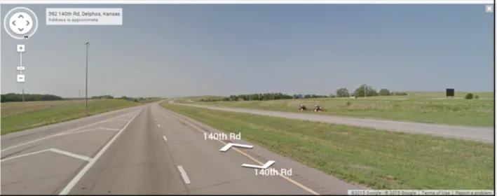
Google Maps and Google Earth® were used to obtain information regarding the presence of lighting at segments because this data is not readily available through KDOT. “Street View” in the Google application enabled zooming in order to determine the presence of a light post. Although the resolution was low in both Google applications, light posts were observed. Figure 3.1 shows the Google Maps application to ascertain the presence of lighting at a segment.

Figure 3.1 Using Google Map to obtain presence of lighting

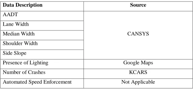
A summary of data sources is shown in Table 3.1. The HSM considers the presence of automated speed enforcement as optional (desired) data. Since Kansas does not have automated speed enforcement, this data was not applicable for Kansas. Once all data were obtained, they were used in accordance with the HSM methodology.

(37)

Table 3.1 Data sources for rural four-lane segments

Data Description Source

AADT CANSYS Lane Width Median Width Shoulder Width Side Slope

Presence of Lighting Google Maps

Number of Crashes KCARS

Automated Speed Enforcement Not Applicable

3.2 Study Segments

The CANSYS database provided a list of rural 4D segments and 4U segments in Kansas. The HSM recommends that segments should be at least 0.1 miles long and contain homogeneous geometry and traffic volume within the length. KDOT uses similar rule of homogeneity for defining their segments within CANSYS database. Using these criterion, a total of 281 4D and 83 4U segments were selected and used for calibration in this study according to the HSM methodology. The number of crashes for all 4D segments was 910 per year, and the number of crashes for 4U segments was 44 per year. Lane width, shoulder width, median width, and side slope were also obtained from the CANSYS database.

Google Maps® was used to show crash locations as well as the beginning and ending of segments, demonstrating that segments were spread throughout Kansas. Figures 3.2 and 3.3 show crash locations at 4D and 4U rural roadway segments in Kansas, respectively. Blue and white markers indicate the beginning and end of segments, respectively, and small dot markers identify crash locations on 4D and 4U highways.

(38)

Legends:

- Beginning of Segment - End of Segment - Location of Crash Figure 3.2 Rural 4D segments and crash location map

(39)

Legends:

- Beginning of Segment - End of Segment - Location of Crash Figure 3.3 Rural 4U segments and crash location map

(40)

3.3 Highway Safety Manual Calibration Procedures for Segments

Prediction of the expected number of crashes for an entity given a set of values for input variables follows a three-step process in the HSM. Beginning with an SPF, CMFs and the calibration factor (C) subsequently follow (AASHTO, 2010). The SPF predicts expected crash frequency as a function of AADT and lane width for roadway segments given basic geometrics and traffic conditions. For example, base conditions for a rural four-lane roadway include 12-foot-wide lanes, 8-foot-12-foot-wide right shoulders (for divided segments), 30-foot-12-foot-wide median (for divided segments), 1:7 or flatter side slope (for undivided segments), paved 6-foot-wide shoulder (for undivided segments), no lighting, and no automated speed enforcement. Expected crash frequency for sites with characteristics differing from base conditions can be computed by multiplying CMFs that represent each type of change. After all available CMFs are considered, calibration factor C is used as the ultimate adjustment for all other differences, known or unknown, measurable or immeasurable, such as climate, driver and animal populations, CRTs, and crash reporting system procedures. Factor C is the ratio of observed number of crashes to expected number of crashes. This building block structure of the HSM predictive methods enables separate calibration (AASHTO, 2010).

Because the SPF carries the most weight in predicting crashes, SPF calibration may be more critical and effective than other modifications. Ideally, base conditions should be the most representative characteristic of a roadway, guaranteeing a sizable sample in order to develop statistically robust models. However, the most representative roadway type may vary by state or region. If the sample size that satisfies the base conditions is small, SPF calibration may not be rigorous or representative enough for a larger population (AASHTO, 2010).

(41)

The standard approach to develop calibration factors in the HSM involves the following steps:

 Identify desired facility types  Select segments among these types  Collect required data for those segments  Apply HSM predictive models

 Compute calibration factors

This research considered rural 4D and 4U segments, and all segments within these categories were selected as analysis locations. Once the site type and locations were selected, methodology given in the HSM was followed for calibration.

3.3.1 Safety Performance Functions

SPFs are regression equations that calculate the dependent variable, or predicted crash frequency, based on independent variables. Because this research focused on utilization of the HSM-specified methods, SPFs in the HSM were used to calculate the number of predicted crashes (AASHTO, 2010).

SPF for a rural four-lane highway segment is estimated as

𝑁_𝑆𝑃𝐹 = 𝑒[𝑎+𝑏×𝑙𝑛 (𝐴𝐴𝐷𝑇) + 𝑙𝑛 (𝐿)] _(3.1)

Where,

NSPF = base total expected average crash frequency for the rural segment, AADT = AADT on the highway segment,

L = Length of highway segment (miles), and a and b = regression coefficients.

(42)

3.3.2 Crash Modification Factors

The SPF was multiplied by CMFs for each independent variable, as described in the HSM (AASHTO, 2010). CMFs only address changes in design and operation characteristics (e.g., lane width and shoulder width) typically under the control of highway engineers and designers. They do not address characteristics such as climate, driver behavior, and CRT (Kweon et al., 2014). Equation 3.2 shows the SPF to obtain predicted number of crashes on 4D and 4U segments in the HSM.

𝑁_{𝑃𝑟𝑒𝑑𝑖𝑐𝑡𝑒𝑑} = 𝑁_𝑠𝑝𝑓 × 1.436 × (𝐶𝑀𝐹₁ × 𝐶𝑀𝐹₂ × … … … . 𝐶𝑀𝐹_𝑖) (3.2) Where,

NPredicted = Adjusted number of predicted crash frequency,

Nspf = Total predicted crash frequency under base condition, and CMFi = Crash modification factors.

A CMF greater than 1.0 indicates an expected increase in crashes, demonstrating that the countermeasure decreases safety in that location. A CMF less than 1.0 indicates a reduction in crashes after implementation of the given countermeasure, demonstrating that the countermeasure increases safety in that location.

Chapter 11 in the HSM provides CMFs corresponding to lane width, shoulder width, median width, and side slope. CMF for the presence of lighting was calculated using Equation 3.3. As recommended by the HSM, default proportions of nighttime crashes in the HSM were replaced by Kansas specific crashes.

(43)

Where,

Pinr = Proportion of nighttime crashes for unlighted segments involving fatality or injury, Ppnr = Proportion of nighttime crashes for unlighted segments involving PDO crashes,

and

Pnr = Proportion of total crashes for unlighted segments that occurring at night. 3.3.3 Calibration Factor

SPFs in the HSM were typically developed using data from jurisdictions and/or time periods rather than where or when such SPFs were desired. For example, default HSM-SPFs for rural multilane highways were developed using data from Texas, California, Minnesota, New York, and Washington from 1991 to 1998. However, the general level of crash frequencies potentially varied substantially from one jurisdiction to another and/or from one year to another due to changes in climate, driver behavior, and CRT and the calibration factor addresses these changes (AASHTO, 2010). Therefore, in order to predict reflecting levels of crash frequencies in jurisdictions and/or years of interest, the predicted number of crash frequencies must be adjusted using calibration factors that are determined for each facility/site type.

Calibration factor (C) was obtained by dividing the number of total observed crashes by the number of total predicted crashes. Observed crash frequencies were obtained from the crash database, and predicted crashes were obtained by the HSM-SPF after applying CMFs. A calibration factor less than 1.0 indicates that the HSM-SPF overpredicted crash frequencies. Therefore, multiplying the factor prediction under base conditions lowers the predictions to match observed frequencies on average. A factor greater than 1.0 indicates underprediction; multiplying the factor increases the predictions to match observed frequencies. Equation 3.4 was used to obtain the calibration factor.

(44)

C =

∑all sites observed crashes

∑all sites predicted crashes

(3.4)

3.4 SPF Development

When a calibration factor obtained according to the HSM methodology underpredicts or overpredicts crashes for a particular location, the HSM recommends development of local jurisdiction-specific SPF. This section describes frequently used approaches that could be utilized in developing a new SPF for a roadway facility.

3.4.1 Poisson Regression Model

A Poisson regression model is a generalized linear model, which allows the mean of a population to depend on a linear predictor through a nonlinear link function. This model, which allows the response probability distribution to be any member of an exponential family of distributions, is appropriate for dependent variables that have nonnegative integer values such as 0, 1, 2, etc. Therefore in most cases, Poisson regression can precisely analyze count data. Miaou and Lum (1993) determined the relationship between vehicle crashes and geometric design features of road segments, such as lane width, shoulder width, horizontal curvature, and lane width, therefore, proposed the Poisson regression model, as shown in Equation 3.5.

P (Yi = yi) = p (yi) =

𝜇𝑖𝑦𝑖𝑒−𝜇𝑖

(45)

Where,

i = A roadway segment (the same roadway segments in other sample periods are considered to be separate roadway segments),

Yi = The number of crashes for a given time period for roadway segment i,

yi = The actual number of crashes for a given time period for roadway segment i,

P (yi) = Probability of crash occurrence for a given time period on roadway segment i, and 𝜇_𝑖 = Mean value of crashes occurring in a given time period as,

𝜇_𝑖 = E (Yi) = 𝜃_𝑖[𝑒∑ 𝑥𝑖𝑗𝛽𝑗

𝑘

𝑗=1 ] _(3.6)

Where,

𝑥_𝑖𝑗= The independent jth variable for roadway segment i,

𝛽𝑗 = The coefficient for the jth independent variable, and

𝜃_𝑖 = Traffic exposure for roadway segment i.

For each roadway segment i, xi independent variables describe geometric characteristics, traffic conditions, and other relevant attributes. Traffic exposure, or the amount of travel during the sample year, can be computed using Equation 3.7.

𝜃_𝑖 = 365 × 𝐴𝐴𝐷𝑇_𝑖× 𝑇% × 𝑙_𝑖 (3.7)

Where,

𝐴𝐴𝐷𝑇_𝑖 = Annual average daily traffic (number of vehicles), T% = Percentage of all vehicles in traffic stream, and

(46)

A Poisson regression model assumes that crash numbers for a given time period for roadway segment (Yi, i = 1,2,3….,n ) are independent of each other and has Poisson distribution with mean 𝜇_𝑖. The expected number of crashes E(y_𝑖) is proportional to motor vehicle travel 𝜃_𝑖. The model ensures that crash frequency is positive, using an exponential function given by Equation 3.8.

𝜆

_𝑖

=

𝐸(𝑦𝑖)

𝜃_𝑖 = exp (xi𝛽) (3.8)

Where,

𝜆𝑖 = Crash-involvement frequency

𝐸(𝑦_𝑖) = The expected number of crashes,

xi = Transpose of covariate vector, 𝜃𝑖 = Amount of motor vehicle travel, and

𝛽 = Vector of unknown regression parameter.

The maximum likelihood method in the SAS GENMOD procedure can be used to estimate parameters of the Poisson regression model for log (μ). One important property of the Poisson regression is that it restricts the mean and variance of the distribution to be equal, written as

Var (yi) = E(yi) = 𝜇_𝑖 (3.9)

Where,

μi= Mean of response variable yi,

E(yi) = Expected number of response variable, and

Var (yi) = Variance of response variable yi.

Using an inappropriate model can affect statistical inference and resulting conclusions. Deviance and a Pearson Chi-square statistic divided by degrees of freedom can be used to detect

(47)

the number of parameters estimated in the model from the total number of roadway segments considered for crash prediction modeling.