Application of Deep Learning to
Brain Connectivity Classification in
Large MRI Datasets
Matthew Leming
A thesis presented for the degree of
Doctor of Philosophy
Department of Psychiatry
University of Cambridge
United Kingdom
June 2020
Acknowledgements
I would like to thank those individuals that contributed to the published and submitted forms of this research, which include Shayanti Chattopadhyay, Li Su, Juan Manuel-Gorr´ız, Simon Baron-Cohen, and, of course, my supervisor John Suckling. I would also like to thank those individuals that contributed through either informal advice and conversations to the development of this work or whose data releases were essential to carrying out several studies, including Sarah Morgan, Richard Bethlehem, Varun Warrier, Lena Dorfschmidt, and Ed Bullmore. And I would like to thank Luca Villa and Ayan Mandal, with whom I have had frequent conversations about neuroscience in general, which helped with my overall understanding of the field.
Declaration
I hereby declare that except where specific reference is made to the work of others, the contents of this dissertation are original and have not been submitted in whole or in part for consideration for any other degree or qualification in this, or any other university. This dissertation is my own work and contains nothing which is the outcome of work done in collaboration with others, except as specified in the text and Acknowledgements. This dissertation contains fewer than 60,000 words excluding appendices, bibliography, footnotes, tables, equations, and has fewer than 150 figures.
Abstract
Title: Application of Deep Learning to Brain Connectivity Classification in Large MRI Datasets
The use of machine learning for whole-brain classification of magnetic resonance imaging (MRI) data is of clear interest, both for understanding phenotypic differences in brain struc-ture and function and for diagnostic applications. Developments of deep learning models in the past decade have revolutionized photographic image and speech recognition, bringing promise to do the same to other fields of science. However, there are many practical and theoretical challenges in the translation of such methods to the unique context of MRIs of the brain. This thesis presents a theoretical underpinning for whole-brain classification of extremely large datasets of multi-site MRIs, including machine learning model architecture, dataset curation methods, machine learning visualization methods, encoding of MRI data, and feature extraction. To replicate large sample sizes typically applied to deep learning models, a dataset of over 50,000 functional and structural MRIs was amassed from nine dif-ferent databases, and the undertaken analyses were conducted on three covariates commonly found across these collections: sex, resting state/task, and autism spectrum disorder. I find that deep learning is not only a method that has promise for clinical application in the future, but also a powerful statistical tool for analyzing complex, nonlinear relationships in brain data where conventional statistics may fail. However, results are also dependent on factors such as dataset imbalances, confounding factors such as motion and head size, selected meth-ods of encoding MRI data, variability of machine learning models and selected methmeth-ods of visualizing the machine learning results. In this thesis, I present the following methodologi-cal innovations: (1) a method of balancing datasets as a means of regressing out measurable confounding factors; (2) a means of removing spatial biases from deep learning visualiza-tion methods; (3) methods of encoding funcvisualiza-tional and structural datasets as connectivity matrices; (4) the use of ensemble models and convolutional neural network architectures to improve classification accuracy and consistency; (5) adaptation of deep learning visualiza-tion methods to study brain connecvisualiza-tions utilized in the classificavisualiza-tion process. Addivisualiza-tionally, I discuss interpretations, limitations, and future directions of this research.
List of Publications
• Leming, M., Su, L., Chattopadhyay, S., Suckling, J. “Normative Pathways in the Functional Connectome.” NeuroImage 184(1): 317-334. 2019.
• Leming, M. and Suckling, J. “Deep Learning on Brain Images in Autism: What Do Large Samples Reveal of Its Complexity?” Proceedings of the 8th International Work-Conference on the Interplay Between Natural and Artificial Computation, Part I (Springer, 2019): 389–402.
• Leming, M., Manuel-Gorr´ız, J., and Suckling, J. “Ensemble deep learning on large, mixed-site fMRI datasets in autism and other tasks.” International Journal of Neural Systems 30(7): 2050012-1–16. 2020.
• Leming, M. and Suckling, J. “Stochastic encoding of graphs in deep learning allows for complex analysis of gender classification in resting-state and task functional brain networks from the UK Biobank.” (Submitted to IEEE Trans. on Pattern Analysis), 2020. (https://arxiv.org/abs/2002.10936)
• Leming, M., Baron-Cohen, S., and Suckling, J. “Single-participant structural connec-tivity matrices lead to greater accuracy in classification of participants than func-tion in autism in MRI.” (Submitted to IEEE Trans. on Med. Imaging). 2020. (https://arxiv.org/abs/2005.08035)
Contents
1 Introduction 1 1.1 MRI . . . 1 1.1.1 Structural MRI . . . 1 1.1.2 Functional MRI . . . 2 1.2 Graph theory . . . 3 1.3 Connectivity . . . 4 1.3.1 Functional connectivity . . . 4 1.3.2 Structural connectivity . . . 6 1.3.3 Multi-slice connectomes . . . 71.3.4 Identification of brain networks . . . 8
1.4 Machine learning . . . 10
1.4.1 Overview . . . 10
1.4.2 Training . . . 10
1.4.3 Overview of machine learning methods . . . 11
1.4.4 Convolutional neural networks to classify graphs . . . 12
1.4.5 Explainable AI and the black box problem . . . 13
vi CONTENTS
1.4.6 Methods of visualizing deep neural networks . . . 14
1.4.7 Machine learning in medical imaging of the brain . . . 17
1.5 Big data in medical imaging . . . 19
1.5.1 Overview . . . 19
1.5.2 Role in machine learning . . . 19
1.6 Connectivity in different cohorts . . . 20
1.6.1 Task fMRI . . . 21 1.6.2 Sex . . . 21 1.6.3 Autism . . . 25 1.6.4 Depression . . . 27 1.7 Research Aims . . . 27 1.8 Thesis outline . . . 28
1.9 Motivation and Themes . . . 29
2 Amassing and processing large datasets 31 2.1 Data acquisition . . . 31
2.1.1 Dataset descriptions and labeling . . . 32
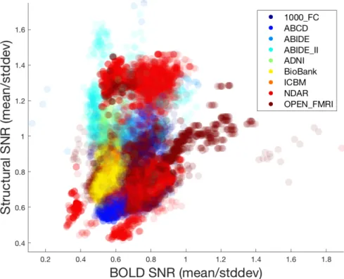
2.1.2 Distribution of data quality . . . 35
2.2 FMRI signal processing toolbox . . . 35
2.3 Dataset counts . . . 36
2.4 Deep learning model . . . 37
2.4.2 Implementation of visualization methods . . . 38
2.5 Use of Connectivity . . . 39
2.6 Practical limitations . . . 40
2.7 Hyperparameter tuning . . . 41
2.8 Note about AUROC and accuracy . . . 43
3 Brain connectivity analysis for mental conditions 45 3.1 Normative pathways . . . 45
3.1.1 Introduction . . . 46
3.1.2 Methods . . . 49
3.1.3 Results . . . 59
3.1.4 Conclusion . . . 76
3.2 A novel structural connectivity metric . . . 77
3.2.1 Introduction . . . 77
3.2.2 Methods . . . 78
3.2.3 Results . . . 80
3.2.4 Discussion . . . 81
4 Ensemble CNNs for connectivity classification 83 4.1 Introduction . . . 83
4.2 Methods . . . 85
4.2.1 Datasets and preprocessing . . . 85
viii CONTENTS
4.2.3 Set division . . . 88
4.2.4 Test set evaluation . . . 88
4.2.5 Experiments . . . 89
4.3 Results . . . 90
4.3.1 Autism vs TD controls . . . 90
4.3.2 Sex . . . 92
4.3.3 Rest vs task . . . 92
4.3.4 Ensemble model limits . . . 93
4.4 Discussion . . . 93 4.5 Conclusion . . . 95 5 Activation maximization 97 5.1 Introduction . . . 97 5.2 Methods . . . 98 5.3 Results . . . 99 5.3.1 Autism vs TD controls . . . 100 5.3.2 Sex . . . 101 5.3.3 Rest vs task . . . 101 5.4 Discussion . . . 102
6 Multivariate class balancing 105 6.1 Introduction . . . 106
6.2.1 Data pre-processing . . . 107
6.2.2 Multivariate class balancing . . . 108
6.2.3 Formalization of multivariate class balancing problem . . . 108
6.2.4 Balancing algorithm . . . 109
6.3 Results . . . 110
7 Salience in brain connectomes 111 7.1 Introduction . . . 111
7.1.1 Network brain function across the sexes . . . 113
7.2 Methods . . . 116
7.2.1 Machine learning . . . 116
7.2.2 Visualization of machine learning results . . . 117
7.3 Results . . . 121
7.3.1 Machine learning . . . 121
7.3.2 Visualization of machine learning results . . . 121
7.4 Discussion . . . 128
7.4.1 Deep learning model . . . 128
7.4.2 Neuroscientific findings of CAMs from vertical filters (from Chapter 4) 130 7.4.3 Neuroscientific interpretations of CAMs from sex classification in UK BioBank . . . 131
7.5 Conclusion . . . 133
x CONTENTS
8.1 Introduction . . . 135
8.1.1 Studies of the structure-function relationship in the brain . . . 137
8.1.2 Experiments . . . 139
8.2 Methods . . . 139
8.2.1 Dataset . . . 139
8.2.2 Pre-processing and feature extraction . . . 140
8.2.3 Machine learning model and training . . . 140
8.2.4 Class activation map analysis . . . 142
8.3 Results . . . 142
8.3.1 Training . . . 142
8.3.2 Class activation map analysis . . . 144
8.4 Discussion . . . 146
8.5 Conclusion . . . 149
9 General discussion 153 9.1 Summary . . . 153
9.2 Big versus small datasets . . . 155
9.3 Psychiatric diagnosis in machine learning . . . 156
9.4 Class balancing techniques . . . 156
9.5 Comparison of machine learning encoding methods . . . 158
9.6 Interpretation of visualization methods . . . 160
9.8 Failed research directions . . . 161
9.9 Future directions . . . 163
Chapter 1
Introduction
1.1
MRI
1.1.1
Structural MRI
The phenomenon of nuclear magnetic resonance (NMR) was originally described in the first half of the 20th century (Purcell et al., 1946; Bloch et al., 1946). NMR refers to the physical observation that atomic nuclei, when held in a strong magnetic field, may be perturbed by a weaker magnetic field and, when released, send out an electromagnetic pulse as the nucleus returns to its original alignment. This outgoing pulse is proportional to the strength of the applied magnetic field, which is the property that MRI takes advantage of to acquire 3D images (Damadian, 1971; Lauterbur, 1973; Mansfield and Maudsley, 1977). By applying and varying magnetic field strengths in unique intensity ranges in three dimensions (thereby assuring that only localized protons with a certain field strength applied will reply to a magnetic pulse) and detecting the output nuclear magnetic resonance strengths, a 3D k-space varying across spatial frequencies can be filled (or, more commonly, many slices of 2D k-spaces that compose a 3D space). By the application of a Fourier transform, a 3D representation of water density in tissue can be derived.
3D MR images can take different forms by varying the repetition time (TR) (or the time between successive pulse sequences applied to a particular slice) and the echo time (TE) (or the time between the delivery of the magnetic pulse and the reception of the echo signal). The most common of these forms are T1- and T2-weighted images. T1, the longitudinal
relaxation time, refers to the time required for shifted electrons to return to equilibrium with the strong magnetic field after the pulse is removed, and can be emphasized in MRIs with short echo and repetition times. T2, the transverse relaxation time, refers to the time taken for excited protons to lose phase with each other, measuring the coherence of nuclei spinning perpendicular to the main magnetic field, and can be obtained with long repetition and echo times. Practically, T1 is useful for viewing brain structure (with cerebrospinal fluid appearing darker and brain matter appearing brighter), while T2 is more often used to view lesions (with fluids appearing brighter). Other variations of 3D MRI can be obtained by varying TE and TR, such as fluid-attenuated inversion recovery (FLAIR) and proton density imaging, but T1- and T2-weighted MRIs are the most commonly used.
The 1990s saw several extensions of MRI into four dimensions, through rapid acquisition of multiple 3D volumes with different settings, that produced a number of new innovations in the field. Most notably, diffusion-weighted imaging, which produces diffusion tensor imaging (Basser et al., 1994), has aided the study of white matter tracts in the brain, while functional MRI (Ogawa et al., 1990) produced a means of studying localized brain function.
1.1.2
Functional MRI
Functional MRI (fMRI) (Ogawa et al., 1990) builds on 3D MRI by taking advantage of the magnetic properties of hemoglobin (Pauling and Coryell, 1936) to show variation in brain metabolism across time. This is called the blood-oxygen level dependent (BOLD) signal, which is believed to be an indirect indicator of brain activity. The use of rapid 3D acquisition allows for the measurement of the BOLD signal within a given period of time. However, due to time constraints, these individual slices are often of lower resolution than typical structural MRI, and even with different optimizations applied, fMRI’s temporal resolution, being limited by acquisition speeds and the haemodynamic response that composes the BOLD signal, is within the range of 1-2 seconds. This puts it at a disadvantage over methods of detecting brain activity, such as EEG, which has a higher temporal resolution, but it is the best means available of studying it in localized areas of the brain, even though the BOLD signal is considered an indirect indication of brain function.
FMRI has not yet found widespread clinical use, but is most often applied in psychological studies, typically either to test brain activation in different psychological tasks, or to compare resting-state brain activity in different populations. Task studies have found that different tasks characterize different localized activations and brain network patterns across different
1.2. GRAPH THEORY 3
populations, but the nature of the tasks, differences in population sample sizes and covariates, and vastly different preprocessing and analysis methods, often make it difficult to compare two different task fMRI studies. The use of resting-state fMRI alleviates the first of these issues, though had been found to have a higher variability than task fMRI when only a single task is considered (Elton and Gao, 2015).
FMRI is hugely affected by confounding factors, notably head motion, which affects the reading of the BOLD signal (Duncan and Northoff, 2013). This has particularly high po-tential to affect the outcomes of studies when motion is measurably different between two populations being studied, which is often the case. While physical constraints and seda-tives may provide a means of reducing motion in the patient, these are either inconsistently applied, undesirable for a study, or ineffective at completely eliminating motion effects. A number of preprocessing steps have been proposed to regress out the effects of motion in the acquired data (Caballero-Gaudes and Reynolds, 2017), including registration of the 3D timepoints, head re-alignment (Goto et al., 2016), wavelet despiking (Patel et al., 2014), and more advanced methods (Kundu et al., 2012, 2013), but because the spin-echo effects of mo-tion on water molecules are extremely difficult to model, none have been able to completely eliminate the effects of motion. While it may be difficult to fully regress, it is possible to detect the amount of motion by measuring the displacement of one 3D slice with its neighbor (Freire et al., 2002). A common practice in fMRI studies is to remove subjects with excessive measured head motion from the study and apply standard motion regression methods to the remaining data.
1.2
Graph theory
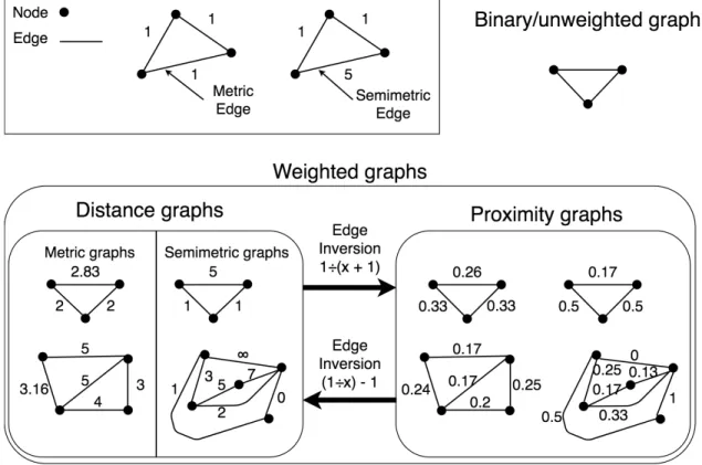
Graph theory is the study of nodes (or vertices) interconnected by edges that compose networks (or graphs). It is used to model many real-world systems, such as airline routes, road systems, and social networks. Graph theory has seen extensive development in the fields of computer science, statistics, and mathematics, and this wide development is often borrowed by other fields to analyze complex scientific data for which a graph representation can be found (Papo et al., 2014). Because of this, graph theory is a favorable means to model and analyze brain networks. This field is often called “connectivity”. For instance, two frequent applications of graph theory to brain connectivity are assessments of node centrality (Zuo et al., 2011; van den Heuvel and Sporns, 2013) (i.e., determining which nodes are “important” in a graph) and community partitioning (Sporns and Betzel, 2016)
(i.e., determining ways to separate networks into smaller subnetworks).
1.3
Connectivity
In brain connectivity, MRI datasets are reduced to a graph representation that is referred to as a “connectome”. In this context, while brain “connections” may represent some type of physiological relationship between two areas of the brain, they may also represent measure-ments of functional or physiological similarity. Other than being a function that reduces an MRI dataset to a network representation, different methods of estimating brain connectivity may have little else in common. In this section, I review different types of connectivity and previous work on identifying subnetworks in brain connectomes.
1.3.1
Functional connectivity
Since its inception, many computational methods have been developed to analyze fMRI data. One such method, functional connectomics (Friston et al., 1993), reduces the dimen-sionality of fMRI datasets to graphs (or networks), comprising nodes, representing brain areas, connected by edges, that represent the relationships between the measured BOLD signals (usually reduced to a timeseries) in these localized areas of the brain. While this dimensionality reduction simplifies the data and does away with a large amount of signal, it does allow for the use of graph theoretical methods, which has been extensively developed in pure mathematics and computer science. Furthermore, depending on the method used to construct the connectome, it allows for the direct analysis of relationships between regions of the brain. This enables the study of brain networks and pathways.
Graph theory metrics, when applied to functional connectomes, can estimates the qualities of brain organization with measurements such as centrality (or “hubness”) (Sporns et al., 2007; Joyce et al., 2010; Lohmann et al., 2010; Rubinov and Sporns, 2010; Tomasi and Volkow, 2010, 2011b; Zuo et al., 2011) and community structure (or “modularity”) (Traag and Bruggeman, 2009; Mucha et al., 2010; Bassett et al., 2013; Sporns and Betzel, 2016). In general, the functional connectome is characterized by high complexity (Sporns et al., 2000; Sporns, 2006), high efficiency (Buzsaki et al., 2004), global and local synchronizability (Masuda and Aihara, 2004), and high levels of clustering with short path lengths (Hilgetag et al., 2000; Stephan et al., 2000; Bassett and Bullmore, 2006), indicating a small-world
1.3. CONNECTIVITY 5
architecture (Milgram, 1967; Watts and Strogatz, 1998). Functional connectomes are also unique to individuals; this is called the connectome “fingerprint” (Finn et al., 2015). Fox et al. (2005) posited that the brain is organized into anticorrelated functional networks distributed over a wide area.
Individual brain networks have been consistently discerned from functional connectivity – for instance, the default mode network (DMN) in resting-state – though there is some disagree-ment as to the makeup and discerndisagree-ment of these networks Stanley et al. (2013). Research in brain networks is often performed with methods other than functional connectivity, such as independent component analysis (ICA). Some brain parcellations model common a-priori networks rather than smaller, anatomical areas of the brain. Discrepancies in brain networks are exacerbated by technical factors such as the parcellation used to derive the network; function-structure couplings (i.e, whether certain functional areas appear consistently in a particular anatomical area); whether the subject was in task or resting state and, if task, which task was performed; and other factors (Power et al., 2011; Sung et al., 2018).
Types of functional connectivity
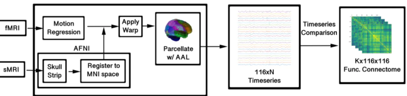
Given a 2D timeseries, composed of a 1D signal for each parcellated area, functional con-nectivity can be derived using one of the many time series comparison metrics available; the output of a connectome parcellation program withN areas andM timepoints is a timeseries of sizeN×M. Using a timeseries comparison metric, this can be transformed into anN×N matrix. Due to its widespread use in other fields, the most commonly favored metric is Pearson correlation, though the use of partial correlation, average mutual information, co-herence, multi-band wavelet correlation, and others, have been proposed, with each having its own features and limitations, such as linearity versus nonlinearity, regression of global signal, and widespread use that contributes to general understanding (Bastos and Schoffelen, 2016). The use of predictive metrics (such as Granger causality (Ding et al., 2006)) may also be applied, but this models a causal relationship between brain regions and is more often referred to as “effective connectivity”, rather than functional connectivity (Friston, 1994; Kriston, 2011).
Different timeseries comparison metrics can lead to the expression of different properties and connectomes with very different topologies; furthermore, differences in the output do-main of different timeseries metrics affect the analysis techniques. For instance, any type of correlation values are between -1 and 1; these negative correlations give rise to a problem
of interpretability that is not easy for neuroscientists to address and which has generated a wide debate in connectomics (Zhan et al., 2017). However, mutual information, another comparison technique, produced values that are above 0, effectively avoiding this issue.
The most common metric of comparison is Pearson’s correlation, which captures the linear relationship between timeseries values. While it is quick to compute and, given its prevalence in statistics, easy to interpret, it also fails to adequately capture nonlinear relationships be-tween timeseries. Mutual information is a common alternative that does capture nonlinear solutions; however, while there is a theoretical basis of mutual information in information theory, there is no standardized way to calculate it on real-world data, leading to a number of different implementations. Partial correlation is a metric that regresses out every other timeseries when comparing two timeseries. It is the inverse of the correlation matrix. A qual-ity of partial correlation is that it effectively regresses the global signal, including unwanted fluctuations in the BOLD signal due to blood flow. However, given too many parcellation areas and too few timepoints, partial correlation may regress out too much of the signal for useful analysis.
These three metrics may also be repeated on the timeseries following a wavelet transform (Patel and Bullmore, 2016); wavelet transforms operate on the signal, producing a decom-position in different frequency bands (requiring information about the repetition time of the MRI when comparing across sites), and, for Qdifferent frequency ranges, this allows for the transformation of an N ×M timeseries into an N ×N ×Q matrix. Often, the analysis of such wavelet correlation matrices are performed on just one of these N ×N matrices, as it is more difficult to interpret a multi-slice matrix as a graph, though more advanced methods allow for the analysis of multi-slice connectomes (Bassett et al., 2013).
1.3.2
Structural connectivity
Tractography and diffusion-based methods
The most well-known structural connectivity methods are based on white matter tract trac-ing between regions (Basser et al., 1994). While this produces the same output format as functional connectivity – an undirected adjacency matrix representing a single subject – they are methodologically very different. Structural connectivity, in its most widely-used form, represents the integrity of white matter fiber tracts. Producing such representations requires diffusion-weighted imaging, as this encodes information about the Brownian motion of water
1.3. CONNECTIVITY 7
molecules, which is directionally restricted by white matter tracts, allowing for the structure of white matter to be inferred (Jones et al., 2013). The strength of the connection can be quantified in several ways, such as the probability of a connection, fiber length, fiber density, or fiber count (Jones et al., 2013; Ji et al., 2014).
Structural covariance
Structural covariance (Wright et al., 1999) is an alternative means of constructing structural brain networks, though it is applied to represent groups, rather than individual subjects. After an N-area parcellation to a group of M structural MRIs, some scalar measurement (such as cortical thickness (Gong et al., 2012)) is estimated for each subject within each parcellation, producing N×M values. Like functional timeseries, these values may then be correlated. This offers a description of how different brain measurements of brain structure may relate to one another across populations.
Structural covariance networks have similar properties to functional connectivity networks, such as small worldness, nonrandom clustering, and modularity. Such properties, however, can also be seen in many real-world networks (Alexander-Bloch et al., 2013a) and may be linked to the tendency of structures to commonly co-vary over short distances (Chen et al., 2008) and occasionally over long distances; for instance, symmetrical regions of the brain, though often spatially disparate, tend to co-vary (Mechelli et al., 2005). Typically, spatial proximity is an indicator of both higher structural covariance between two regions and correlated functional activity (Salvador et al., 2005; Honey et al., 2009; Alexander-Bloch et al., 2013b).
1.3.3
Multi-slice connectomes
Given the diverse means available of analyzing timeseries, some are able to produce a multi-slice functional connectome (i.e, a K ×N ×N matrix, as opposed to a single-slice N ×N matrix). Such connectomes play an important role in this thesis.
Research in the analysis of multi-slice matrices is more difficult due to the complexity of analysis and visualization of an added dimension, and the under-development of it in other fields compared to single-slice graphs. Because of the more diverse means of calculating timeseries comparisons, multislice analysis is more developed in functional connectivity than
in structural connectivity. Even with developments that show high potential for multi-slice matrices, such as multi-level wavelet correlation (Patel et al., 2014; Patel and Bullmore, 2016) and dynamic functional connectivity (Calhoun et al., 2014; Calhoun and Adali, 2016; Preti et al., 2017), a typical practice is often to average such matrices into a single one, or to select a single timeseries comparison, or to analyze timeseries comparisons separately Achard et al. (2006); Achard and Bullmore (2007); Mucha et al. (2010).
Wavelet correlation (Bullmore et al., 2004; Achard et al., 2006; Achard and Bullmore, 2007; Skidmore et al., 2011) is the correlation of different scales in the wavelet decomposition of an fMRI timeseries, which allows for the building of a multislice connectome representative of the whole timeseries. Though it is more common to use a wavelet decomposition (Bullmore et al., 2004; Zhang et al., 2016b) for preprocessing (Patel et al., 2014), they have been used to derive multislice connectomes by correlating regional timecourses in different frequencies (Achard et al., 2006; Thompson and Fransson, 2015); most often, however, after deriving such a multislice connectome, slices are analyzed independently (Berlingerio et al., 2011).
1.3.4
Identification of brain networks
The application of graph theory to MRI data has led to the identification of anatomical and functional brain networks. This can be applied to the context of structural connectivity, which most often refers to white matter networks, but is most often used in reference to functional connectivity, indicating groups of disparate brain areas that are functionally simi-lar under certain tasks (Bressler and Menon, 2010). These networks have been characterized by general, global properties, quantified by graph theoretical measurements, as well as iden-tification of subnetworks in functional MRI data that have been associated with different properties. While identification of these networks is subject to the selected psychological task, brain parcellation, and analysis methods, a few common networks are consistently identified.
Common brain networks
The identification of brain networks in functional data in the literature is often dependent on the aim of the study and datasets analyzed. For instance, Sung et al. (2018) identified 111 brain networks related to psychometric parameters, while Smith et al. (2009) identified just 10. Greene et al. (2018) listed 10 “canonical” networks: the medial frontal, frontoparietal,
1.3. CONNECTIVITY 9
default mode, motor cortex, visual A, visual B, visual association, salience, subcortical, and cerebellum. Generally, the networks discussed the most in literature of resting-state and task fMRI are the default mode (Raichle et al., 2001), executive control, salience (Seeley et al., 2007), dorsal attention, and ventral attention networks (Vossel et al., 2014).
Issues in quantifying brain networks
Atlas-based parcellations are used to derive a brain network using predefined ROIs, defined either by anatomical regions, common functional areas, or randomly. Brain networks are affected by the selection of the parcellation atlas to a large extent (Yao et al., 2015). This is true in a trivial sense, as finer parcellations are able to quantify finer sections of the brain and lead to more detailed networks, but atlases also affect measurements derived from such networks; Wang et al. (2009) found that small worldness is substantially different depending on the selected parcellation atlas, and Zalesky et al. (2010) found that node scale in randomly parcellated structural connectomes affected global connectivity measurements substantially. Brain network estimation can be affected as well by spatial variability of functional hubs (Mueller et al., 2013) (which can be addressed by subject-specific parcellations (Dhillon et al., 2014)), inaccuracies in spatial alignment of the parcellation atlas (Smith et al., 2011; Allen et al., 2012), and the natural variability of cortical area size, which can vary by twofold or more across individuals (Amunts et al., 2000; Glasser et al., 2016; Bijsterbosch et al., 2018).
As one way to account for variability of functional locations in subjects, cluster-based parcel-lations have been proposed. In cluster-based parcelparcel-lations, the parcellation is developed for the individual based on where activity is localized in the brain (Yao et al., 2015). Groupwise comparisons across personalized parcellations has its advantages and disadvantages; under-lying networks are captured more effectively in personalized parcellations, but the fact that certain parts of the functional network are located in different anatomical areas may also be of interest, and this information is lost in personalized parcellations. Bijsterbosch et al. (2018) noted that differences in connectivity may indicate more about anatomical layout of functional regions than about differences in connectivity between those regions.
In order to address the shortcomings of hard parcellation techniques that fail to account for individual variations in functional hub locations and overlapping hubs, more advanced ICA parcellation techniques are able to parcellate overlapping areas (i.e., “soft” parcellations) using dual regression analysis or back projection (Calhoun et al., 2001; Filippini et al., 2009), which obtain subject-specific spatial maps using a group ICA maps (Bijsterbosch
et al., 2018). Seed correlation analysis is also used as a means of studying brain networks; however, this requires a prior assumptions about the location of the network, as one must predefine the areas to correlate.
Besides parcellations, another issue that can affect the quantification of brain networks is anatomical factors that confound the BOLD signal itself. Functional connectivity may increase as the result of non-neuronal fluctuations in the BOLD signal, such as blood pressure, head motion, or respiratory activity (Caballero-Gaudes and Reynolds, 2017). In most cases, the magnitude of changes from these confounding factors are greater than what one can expect from neuronal fluctuations in the BOLD signal, and so simple options such as wavelet despiking (Patel et al., 2014) or other bandpass filtering methods may be adopted. However, it is difficult to remove this global signal, and even with advanced preprocessing techniques (Kundu et al., 2012) and preventative efforts, trace effects of these non-BOLD artefacts usually remain.
1.4
Machine learning
1.4.1
Overview
“Machine learning” (ML) refers to a number of statistical models for identifying and gen-eralizing patterns in data. Machine learning can either be unsupervised, which consists of methods of clustering unlabeled data (for instance, identifying friend groups in a social net-work, or communities in a brain network), or supervised, in which a model learns to associate patterns in the data with different labels (for instance, distinguishing between images of cats and dogs). This thesis focuses on supervised learning.
1.4.2
Training
In the typical supervised learning paradigm, one has a collection of data and a selected model. The data is then divided into two parts: training and test data. Most often, the majority of the data is used for training. The model is then “trained” on the training data for a number of iterations, often with datasets grouped into smaller batches. One update of the model’s parameters over a single batch is called an “iteration”, and when the model iterates over enough batches such that it has seen the entire training set, one “epoch” has
1.4. MACHINE LEARNING 11
been completed. After the training algorithm has finished a set number of epochs, or has achieved 100% classification accuracy on the training set, it is then evaluated on the test set, and the final accuracy is reported.
One problem in machine learning is overfitting, in which the model overfits on the training set, such that it fails to generalize underlying patterns in the data. This is often the result of a model with too many parameters being trained on a training set that is too small, and thus the model is inappropriate for the data. It may also result from overtraining the model. To address this, data may be divided into three sets: training, test, and validation sets. The model does not train explicitly on the validation set, but it uses the validation set to measure accuracy at each epoch, stopping either when an accuracy threshold is reached, or saving a copy of the model on the iteration that produced the highest accuracy on the validation set.
Underfitting during training – in which the model fails to achieve 100% accuracy on the training set – is another problem, and is typically the result of too few parameters in a model, or patterns in a dataset too complex to effectively be characterized by the selected model (for instance, linear regression is likely insufficient to distinguish between pictures of cats and dogs).
Accuracy achieved on a particular division between training, test, and validation data is not deterministic, and it may change if that division changes. Furthermore, some machine learning models (especially neural networks) have stochastic elements that affect the final outcome of the model, even if the divisions remain the same. For this reason, a typical strategy in machine learning studies is to employ cross-validation (Kohavi, 1995), in which a number of independent models (usually a minimum of 10) are trained on different divisions of the data, with the divisions being deliberate such that each datapoint is included equally as often in the training, test, and validation sets. Another form of cross-validation, called leave-one-out testing, is typically employed for much smaller datasets; for a dataset of size n, n independent models are trained on a training set consisting of n−1 datapoints, then evaluated on the one missing datapoint.
1.4.3
Overview of machine learning methods
Unsupervised machine learning methods refer to a number of techniques that may be applied to data without the need for labels, and these methods may be used for applications such as cluster identification (i.e., K-means clustering). Two popular unsupervised deep learning
models are Restricted Boltzmann Machines (RBMs) and variational autoencoders, which are used for data dimensionality reduction.
Support Vector Machines (SVMs) are supervised machine learning models capable of per-forming linear classification of high-dimensional data. SVMs find the best-fit linear division that separates data into two classes, possibly after artificially raising the dimensionality of this data. However, SVMs are only capable of finding linear divisions in data, usually failing to classify complex data such as photographic images.
Neural Networks refer to a number of models inspired by studies of neurons. Neural networks consist of layers of perceptrons, or units that receive a number of inputs and produce a single output. Deep learning is a subfield of machine learning that refers to the use of neural networks with different layers. Neural networks are particularly useful for characterizing complex and high-dimensional data, though extremely large amounts of data are necessary to train a neural network without overfitting. While neural networks have been the subject of research for decades, they were quickly popularized by the method of efficiently training neural networks (Hinton et al., 2006) and the subsequent display of their efficacy in the ImageNet competition (Krizhevsky et al., 2012). Since then, deep learning has been applied to many other fields of research, including MRI analysis.
In modern deep learning, two types of neural networks are very often used. Recurrent Neural Networks (Lipton, 2015) (RNNs) are particularly powerful deep learning models that use, as part of their input, the model output from previous data inputs. As such, they are best for learning sequences, such as semantic sentence interpretation (Karpathy and Fei-Fei, 2014). Convolutional Neural Networks (LeCun et al., 1999) (CNNs) are a powerful model for classifying images and videos, which encode the spatial organization of data by convolving adjacent pixels in successive layers, creating an abstract representation of objects in the process. This thesis employs convolutional neural networks extensively.
1.4.4
Convolutional neural networks to classify graphs
While the most popular application of CNNs has been in classifying 2D images (Krizhevsky et al., 2012), there has been a particular effort in recent years to adapt them to other kinds of data, such as 3D images (Maturana and Scherer, 2015), video (Karpathy and Fei-Fei, 2014), and audio-to-text conversion (Lipton, 2015). Because of their wide applicability in representing data such as proteins and social networks, much work has been done on
clas-1.4. MACHINE LEARNING 13
sifying connected networks, including whole-graph classification, clustering, and node-wise classification (Bruna et al., 2014; Defferrard et al., 2016; Hamilton et al., 2017; Hechtlinger et al., 2017; Kipf and Welling, 2017; Nikolentzos et al., 2017). Graph classification is typ-ically performed in one of three ways: graph kernels (Jie et al., 2013; Kriege et al., 2019; Nikolentzos et al., 2019), translating the graph to another representation (such as an image) before classifying it with a CNN (Tixier et al., 2017), or directly with convolutional neural networks (Kawahara et al., 2017).
Convolutional neural networks (CNNs) adapted for graphs have potent applications in the classification of brain connectomes. While other machine learning (ML) models have been developed for analyzing graph data (Jie et al., 2013; Kriege et al., 2019), they have often been designed to characterize general networks (such as social networks) rather than fixed-node matrix representations, and so are not ideal for brain connectomes. With its utilization of powerful deep learning structures (Kawahara et al., 2017; Brown et al., 2018), however, CNNs are among the most promising ML tools for the diagnosis and prognosis of neurological and mental health disorders using graph representations of the structure and function of the brain. This thesis largely focuses on the adaptation of CNNs to classify graphs.
1.4.5
Explainable AI and the black box problem
A common problem in deep learning is the “black box” problem. A black box is any system that receives an input and outputs a signal without knowledge of its internals, which are abstracted from users. Deep learning models, which often require millions or tens of millions of parameters, are abstracted from human understanding by their own complexity and are thus considered black boxes.
While the black box problem does not directly affect the performance of deep learning models, it creates difficulties when verifying whether a model is focusing on signal or confounding factors. In a well-known instance, Ribeiro et al. (2016) discussed a problem in which a classifier learned to reliably distinguish between pictures of wolves and huskies. However, a proposed explanation of the classifier revealed that, since wolves were mostly imaged with snow in the background, the classifier focused on snow rather than the face of the wolf. They concluded that, in spite of high accuracy, this would not be an appropriate classifier to rely on in a real-world setting.
classification accuracy. The need for explainable machine learning models in a clinical setting has previously been discussed (Gottesman et al., 2019). Clinicians need to fully understand the decision-making process of an automated diagnosis if they are to eventually rely on it. AI models that make a linear, understandable decision-making process are called “expert systems”. These often rely on human-readable information, such as the diagnostic history of an electronic health record. However, such systems would not be capable of making use of more complex datasets that are not always human-readable, such as medical images or genetic records.
Deep learning models have been shown to be capable, at least to a degree, of making sense of complex datasets, in a way that an explainable expert system (Gottesman et al., 2019) would not, in applications like whole-brain MRI diagnostics (Kawahara et al., 2017; Khosla et al., 2018; Leming and Suckling, 2020a,b)). Unlike expert systems, deep learning models’ decision-making processes are too complex for human understanding (i.e., the black box problem). Because of the need for clinicians to explain their decisions, this would make deep learning models of limited value. There has been great effort in visualizing deep learning models in other contexts in the hope of making them explainable. These methods include occlusion, gradient class activation mapping, and activation maximization (Zeiler and Fergus, 2013). While these methods fail to reveal the exact decision-making process used to make classifications, they are capable of showing which parts of the input data are taken into account for the classification. Use of such techniques can make deep learning models more explainable, and thus more useful in an eventual clinical context. But while such methods help explain machine learning models, the full extent of these techniques, and the exact interpretation of any visualization techniques in a scientific context, is still the subject of ongoing research.
1.4.6
Methods of visualizing deep neural networks
The black box problem has motivated a sub-field of research into methods of analyzing and visualizing deep learning models. Most of these techniques were originally developed for 2D image recognition and adapted later to abstract data types. The interest in visualiza-tion methods has motivated different sub-fields of deep learning, such as generative models (Goodfellow et al., 2014), unsupervised object localization (Zhou et al., 2015b; Oquab et al., 2015; Cinbis et al., 2015; Pinheiro and Collobert, 2015; Bergamo et al., 2014; Oquab et al., 2014), and deconvolutional neural networks (Zeiler et al., 2010).
1.4. MACHINE LEARNING 15
Of particular interest in this thesis are those methods that show which parts of input data contribute to classification accuracy – i.e., salience – with the aim being that this elucidates group differences, as well as methods that analyze how the machine learning model itself sorts large datasets during classification, in order to quantify whether a classifier focuses on signal or confounding factors. Three general methods are discussed here: class activation maps, occlusion, and activation maximization.
Class activation maps
Class activation maps (CAMs) measure the influence of localized areas of input on the final accuracy calculation (i.e., “salience”). In the context of photographic image recognition, this is usually interpreted as a measurement of human fixation; for instance, in a classifier that distinguishes between pictures of cats and dogs, the CAM should highlight the shape of the cat or dog in the input image. In its earliest iteration (Simonyan et al., 2014), CAMs were estimated as the derivative of the deep learning function with respect to the input image, approximated as a first-order Taylor series. This, in effect, showed the degree to which each part of the input image altered the final classification. However, the first implementations of CAM estimation offered noisier results before algorithmic improvements were developed. Zhou et al. (2015a) developed CAM estimation further with an algorithm that was more effective at object localization but was only used for specialized CNNs with no fully-connected layers. The later innovation of Selvaraju et al. (2017) generalized this to Guided Grad-CAM, a version of this class activation mapping algorithm that could be applied to a wider variety of deep learning models.
Developments in CAM estimation have re-formed it into an object segmentation tool (Zhou et al., 2015a). Many later developments (Li and Yu, 2018) expanded on it by employing contour-based methods for object segmentation. However, when applicable deep learning models are adapted to other, abstract data types, such object-segmentation-focused salience detection may not be ideal. The parts of input data that affect the output the most would likely not be able to be clustered together in the way objects in 2D images are, as other data may be more abstract than 2D objects. This thesis makes extensive use of CAM algorithms, but because of the irrelevance of object segmentation to brain connectomes, I opt for an earlier implementation (Selvaraju et al., 2017), Guided Grad-CAM, rather than the current state-of-the-art.
respect to a class) of a neural network with respect to the feature maps of a convolutional layer. The gradients are then average-pooled. This represents the salience of particular feature maps for a particular class. A weighted combination of all of these forward activation maps are then added and followed by a rectified linear unit (ReLU, i.e. the absolute value), to obtain a coarse heat map of the same size as the convolutional feature maps (Selvaraju et al., 2017).
Occlusion
Occlusion (Zeiler, 2012) consists of occluding local areas of data and testing which of these lowers classification accuracy the most, effectively showing which areas of the image are most important in this classification. Like CAMs, it is a salience detection technique, and it is advantageous in that it more directly tests for salience. Unlike CAMs, occlusion does not actually involve direct analysis of deep learning parameters at all, but instead works by editing input data; this makes it an applicable method for analyzing black box models in general.
Occlusion can have several variations that have been applied creatively to deep learning: Zhou et al. (2015b) proposed an interesting variation on occlusion, in which the the pixel of an input image that caused the least accuracy was erased until the image was inaccurately classified, and Bergamo et al. (2014) used it as a means of unsupervised object segmentation. However, occlusion is also more computationally intensive than CAM estimation, somewhat limiting its use. Furthermore, the elimination of certain parts of input data may cause the deep learning model to act unpredictably, as it is known that random noise as inputs may output unpredictable results in deep learning models (Szegedy et al., 2014; Goodfellow et al., 2015).
Activation maximization
Activation maximization (Erhan et al., 2009) consists of recording which input data maximize which units in a particular hidden layer of a deep learning model. Typically, one finds the activation maximization of convolutional layers rather than dense layers, as convolutional layers maintain a level of stratification that helps with analysis; for instance, activation maximization of convolutional layers in 2D image recognition can render visuals of abstract shapes and textures of particular input objects within the network. Activation maximization
1.4. MACHINE LEARNING 17
is used to assess how data is organized by the model; for instance, certain subclasses of data are often found to maximally activate different filters in convolutional layers.
1.4.7
Machine learning in medical imaging of the brain
Machine learning has been applied to medical imaging since the 1990s (Zhang et al., 1994), though in more recent years, the industrial deep learning boom has substantially affected medical imaging; the number of publications about machine learning in medical imaging has increased substantially since 2012, with CNNs being the most published about by far (Litjens et al., 2017; Shen et al., 2017a).
Machine learning has been applied to medical imaging for segmentation (Perone and Cohen-Adad, 2019), detection (Tajbakhsh et al., 2015; Tajbakhsh and Liang, 2015; Shin et al., 2016), object classification (Singh and Singh, 2017), and single-subject phenotypic classi-fication (Arbabshirani et al., 2017). Such applications may generally be divided into two categories: ones for which human experts can achieve near-perfect accuracy, and ones which cannot due to the non-discovery of consistent biomarkers. The first category tends to see applications related to image segmentation, such as skull-stripping and tumor segmentation, and even extends into cancer diagnoses (Munir et al., 2019) by analyzing images of tumors or cells; because expert human interactors can achieve near-perfect accuracy with such im-ages, it is established that the necessary information to succeed at the classification task is present in the given dataset. In the second category are image-based diagnostics, often of degenerative or mental disorders, for which human interactors cannot readily make a suc-cessful classification given this data, since the given data is usually not the primary source of such a diagnosis in the first place. For instance, clinicians and radiologists would not di-agnose autism based on brain images, but rather by behavioral markers; thus, it is unknown whether a biomarker exists for autism (Plitt et al., 2015). The present thesis largely focuses on single-subject phenotypic classification using MRIs, which is in the latter category.
Several different classes of machine learning models are in popular use in medical imaging; however, because of their applicability to images, CNNs are a popular choice. According to Litjens et al. (2017), “out of the 47 papers published on [whole-image] classification in 2015, 2016, and 2017, 36 are using CNNs, 5 are based on [autoencoders] and 6 on RBMs”. A review of more years in Arbabshirani et al. (2017) also revealed a widespread use of SVMs, which are more applicable to smaller datasets and suffer less from the black box problem, though SVMs require specialized feature extraction methods, which are often study-specific,
and are often unable to characterize nonlinear patterns in data.
Machine learning studies in brain connectivity have been used for single-subject classification of bipolar disorder, attention deficit hyperactivity disorder (ADHD), mild cognitive impair-ment (MCI), schizophrenia, autism, attention deficit hyperactivity disorder (ADHD), and Alzheimer’s disease (AD) (Du et al., 2018), with studies variously using functional and struc-tural data for classification, depending on the task. Certain disorders, such as autism and ADHD, are mainly characterized by behavioral symptoms, with structural and functional brain differences still being an active area of research. However, even these behavioral symp-toms are difficult to characterize; individuals with autism are not characterized by the same profile, and their symptoms are known to change over time (Lord et al., 2000). The causes of ADHD are still unclear and are likely a number of possible factors, including heredity, brain chemistry, and malnutrition (Biederman, 2005; Dey et al., 2014). Naturally, an incomplete understanding of the disorders themselves does not help with the technical difficulties of classifying images of the brain.
Most of these studies rely on small training datasets. As noted by Arbabshirani et al. (2017) and Katuwal et al. (2015), machine learning models for whole-brain MRI classification generally perform better on small, single-site datasets than on large, mixed-site datasets. This would seem to contradict the conventional wisdom in machine learning that larger training datasets aid model performance. A thorough explanation of this phenomenon has not been offered, but it is typically assumed that mixed-site datasets add confounding factors and variations that are difficult for a model to characterize.
The shortage of health data to aid in machine learning algorithms has led to several efforts in industry at amassing data already present in health records, such as Google’s Project Nightingale (Copeland, 2019) or IBM Watson Health’s partnerships with hospitals (Quach, 2018), though such efforts are routinely plagued by controversy, either due to concerns with diagnostic accuracy (IBM Watson) or data privacy (Project Nightingale). The collection of larger datasets in the research world, such as UK BioBank, holds more promise for studies of big data in the near future.
1.5. BIG DATA IN MEDICAL IMAGING 19
1.5
Big data in medical imaging
1.5.1
Overview
Like many biological applications, machine learning studies in MRI are limited by sample size, as MRIs are comparatively expensive and labor-intensive to acquire. With growing interest in big data in MRI (Smith and Nichols, 2018), wider initiatives to acquire large datasets has allowed for training sets in the hundreds (Abraham et al., 2016) or thousands (He et al., 2018), though even these are orders of magnitude smaller than those used in mainstream computer vision (Wu et al., 2019).
1.5.2
Role in machine learning
There have been methods of overcoming the limitation of small sample sizes in medical imaging, such as data augmentation (Hussain et al., 2017), the use of leave-one-out classifiers (Anderson et al., 2011b; Jang et al., 2017), the use of simulated data (Meszl´enyi et al., 2017), or the development of methods that specialize in training on lower sample sizes (Liu et al., 2014; Akkus et al., 2017; Gibson et al., 2018; Han et al., 2017; Shen et al., 2017a). However, Arbabshirani et al. (2017) observed that most results that showed extremely high accuracy (> 90%) were most often performed on samples of less than 100. This could be due to overfitting of newly developed models, homogeneity of samples, the use of leave-one-out classification (which, though it may seem appropriate for small datasets, can prove statistically unsound (Kohavi, 1995)), or unknown factors. In any case, this brings into question the generalizability of many such models, and it is likely another expression of the statistical problems associated with low sample sizes (also called “power failure”) in neuroscience (Button et al., 2013; Nord et al., 2017).
This necessitates the use of big datasets. In recent years, this has become a more viable option, as there have been several larger initiatives – for instance, the UK Biobank and ABCD – that have collected thousands of datasets from different facilities that centrally work to minimize site differences and make the data as high-quality and homogeneous as possible. The UK Biobank is especially notable for housing extremely detailed metadata about its subjects, allowing for many big-data psychological studies to be performed on the basis of this metadata alone. Such large databases, however, can be lacking in variety of patients with a clinical diagnosis that is often of particular interest to researchers, though
there are several medium-sized (100< N < 5000) databases that are dedicated to the study of particular disorders (i.e., ADNI for Alzheimer’s and ABIDE for autism).
Large imaging databases are often composed of smaller batches collected by individual re-search groups, which are then amalgamated in repositories, such as NDAR and OpenfMRI. These small MRI datasets, however, often have variations that make it extremely difficult to compare subjects in cross-dataset studies. Such differences are not only limited to MRI hardware, parameter, and population differences, but subtle variations in clinical and diag-nostic practices depending on the disease being studied, and preprocessing practices of the holding database. Furthermore, standard practices in brain imaging often calls for a level of human interaction, if only to perform quality control, when preprocessing data, and for collections of this size such standard preprocessing practice would not be viable.
Nonetheless, noisy repositories, in aggregate, house much data of interest, and though the many factors noted above may make it impractical to compare them using conventional methods, deep learning was designed to classify such data with high levels of noise and variation. Deep learning does not resolve all such concerns – for instance, one has to be sure that high accuracy is not simply due to gross imbalances in classes or site differences – but, in theory, it does lessen the need to explicitly model and regress artifacts such as motion or signal weakness, as long as the model is unable to utilize such factors to improve classification accuracy.
1.6
Connectivity in different cohorts
Brown and Hamarneh (2016) provides an overview of previous efforts in brain connectome classification on different phenotypic groups. A direct comparison between deep learning studies is complicated by differences in machine learning models; differences in datasets; preprocessing practices; division between training, test, and validation sets within the same dataset; and differences in metrics used to validate one’s machine learning model. In this section, I summarize previous efforts to classify based on phenotypes considered in the present work (sex, task, autism, and depression); when such studies are sparse or nonexistent, I discuss factors that would likely affect such studies.
1.6. CONNECTIVITY IN DIFFERENT COHORTS 21
1.6.1
Task fMRI
The functional differences found between task-based and resting-state fMRI may be among the most consistent occurrences in fMRI studies. Corbetta and Shulman (2002) first discov-ered the dorsal and ventral attention networks (Vossel et al., 2014), which were respectively concerned with voluntary focus on features and switches in attention or unexpected stim-uli. As noted by Fox et al. (2005), when performing simple memory tasks in a fMRI, the response commonly observed is increased activity in certain frontal and parietal cortical re-gions (Cabeza and Nyberg, 2000; Corbetta and Shulman, 2002) and decreased activity in the posterior cingulate, medial and lateral parietal, and medial prefrontal cortex (Gusnard et al., 2001; Simpson et al., 2001; Shulman et al., 1997; McKiernan et al., 2003; Mazoyer et al., 2001), which form the default mode network; the intensity of this response was proportional to the intensity of the task. Fox et al. (2005) identified two widely distributed, anticorrelated networks in the brain that exist in the resting state but intensify during tasks.
The default mode network has been consistently identified as a marker of resting-state con-nectomes since it was first described in Raichle et al. (2001), and other brain networks, including some emblematic of particular tasks, have been identified as well (Smith et al., 2009). Using fMRI and diffusion-weighted MRI, Yoldemir et al. (2015) distinguished, with 79% accuracy, between seven functional tasks using the fMRI timeseries. On the whole, clas-sification of resting-state and task-based fMRI is underexplored, though Zhang et al. (2016a) recently used sparse representations to distinguish between task- and resting-state fMRI in the Human Connectome Project data, achieving 100% accuracy and distinguishing between subjects by identifying the presence of the default mode network, though this was done on a dataset consisting of only 60 subjects (even though the data collected on each subject was robust and detailed). There has also been work in using deep learning to decode different brain states in individuals (Koyamada et al., 2015), and Li and Fan (2018) creatively applied recurrent neural networks to decode brain states in single-subject fMRI as they changed over the course of a timeseries.
1.6.2
Sex
Evaluation of male-female brain differences are of general and widespread interest in neu-roscience, but this has uniquely complicated the subject: the frequency with which it is studied, combined with the statistically unsound use of small sample sizes (Button et al.,
2013; Nord et al., 2017) in studies that use different analytical methods, has created a very inconsistent picture across the board with regards to brain functional and structural differ-ences between sexes; another view of this, however, is simply that male-female differdiffer-ences are highly complicated and the literature reflects that (Ruigrok et al., 2014).
Functional differences between the sexes are debated and findings generally vary, depending on which aspects of it are studied. A review by Sacher et al. (2013a) cited evidence for functional sex differences in emotional and visuospatial processing, but noted that, up to that point, it was rarely considered as a covariate in fMRI studies, and thus more rarely in resting-state fMRI. Noted differences in emotional and visuospatial processing include arousal differences in the bilateral amygdala and hypothalamus (Hamann et al., 2004; Takahashi et al., 2006; Mackiewicz et al., 2006), the right cerebellum, and the posterior and superior temporal sulcus (Takahashi et al., 2006), as well as hemispheric differences, in response to various emotional stimuli. Men and women also differed in right hemisphere activation in response to visuospatial tests (Gur et al., 2000), and differing activations in the superior parietal lobule and the inferior frontal cortex in response to mental rotation tasks (Hugdahl et al., 2006). In a task in which subjects were presented with emotional faces, men showed higher activation in limbic and prefrontal regions and women higher activation in the right subcallosal gyrus (Fusar-Poli et al., 2009). In response to angry and fearful faces, men show higher activation than women in the visual cortex and the anterior cingulate gyrus (Fischer et al., 2004).
Later studies were performed on large samples of resting-state data rather than smaller sam-ples of task fMRI with different emotional stimuli, mitigating the concerns raised in Button et al. (2013) and Nord et al. (2017). Sex differences have been analyzed in large-sample studies of children and adolescents (Gur and Gur, 2016; Gennatas et al., 2017; Wierenga et al., 2017) and the release of large samples of data in the UK Biobank (Ritchie et al., 2018) (2750 females and 2466 males). (Because this work uses both resting-state and task fMRI, it is reasonable to include both of these in my analysis and hypothesis formation.) High-sample-size studies of resting-state fMRI differences between sexes have not typically implicated differing activations in very localized portions of the brain; generally, however, studies have reported, through different measurements, higher local functional connectivity in women than in men (Tomasi and Volkow, 2011b; Gur and Gur, 2016), though different analytical methods can also make these studies particularly tricky to compare, since indi-vidual studies report arbitrary graph-theoretical measurements or different network ROIs in seed-based analysis.
1.6. CONNECTIVITY IN DIFFERENT COHORTS 23
Unlike function, differences in brain structure between females and males has been exten-sively documented (Ruigrok et al., 2014), both in the developing brain and later in life. Earlier, smaller-scale studies reported that, in the beginning of life, one-year-old boys have bigger brains by about 10 percent, but girls have bigger structures in the brain stems (Giedd et al., 1997) (50 males and 70 females, aged 3–18), and in both sexes the right hemisphere is generally bigger than the left (Baibakov and Fedorov, 2010) (30 males and 30 females, age 12). The sizes of structures are not proportionally bigger across age and sex (allom-etry) (Giedd et al., 2012). Development of certain structures, such as the amygdala and hippocampus, are different in early adolescent years for females and males (Uematsu et al., 2012) (58 males, 53 females, studied from 1 month to 25 years).
Among the most notable findings of large-scale studies of the developing brain, which repre-sent samples of total size 1929 males and 2065 females aged 3 to 23 years (of whom 745 males and 826 females were analyzed functionally (Gur and Gur, 2016)) were the following: (1) a steeper increase in white matter volume in males than in females during puberty, especially in the frontal lobe (Lenroot and Giedd, 2006; Gur and Gur, 2016); (2) bilaterally larger hip-pocampal volume in females after puberty, correlated with memory tests, and equal volumes before (this effect was not seen in the amygdala, however) (Gur and Gur, 2016); (3) in their resting-state functional networks, when they were separated into modules, males showed higher between-module connectivity and females showed higher within-module connectivity (Gur and Gur, 2016); use of SVMs to classify males and females achieved 63% accuracy using only their cognitive profile but 71% accuracy using functional connectivity data (Gur and Gur, 2016), improving on a previous accuracy of 65% accuracy for a similar age group based on functional data from the human connectome project (Casanova et al., 2012) (74 females and 74 males, age 21); (4) the functional connectome shows greater modularity in females and the structural connectome has greater modularity in males (Gur and Gur, 2016); (5) Throughout the brain, females have lower gray matter volume but higher gray matter den-sity than males (Gennatas et al., 2017); (6) with regards to the volume of several key brain structures, including cerebral white matter and cortex, hippocampus, pallidum, putamen, and cerebellar cortex, males showed significantly greater variance than females (Wierenga et al., 2017). Many of these results were supported by an earlier study (Tomasi and Volkow, 2011a) that used a notably large sample size of young adults (336 females and 225 males, aged 18–30 years), finding that women have higher local functional connectivity density and higher gray matter density than men.
2466 males, aged 44 to 77 with a mean of 61.7, found that males have higher brain volumes, surface areas, and white matter fractional anisotrophy, whereas females have higher cortical thickness and white matter complexity. With regards to resting-state functional connectivity, females had stronger connectivity in the default mode network and stronger connectivity for males in the sensorimotor cortices; this may be another expression of the findings of Gur and Gur (2016) and Tomasi and Volkow (2011b) with regards to females having higher within-network/local connectivity (considering the default mode network is one of the most prominent networks in the brain), but given that the results are presented differently, it remains difficult to tell. Supporting the findings of a younger cohort in Wierenga et al. (2017), males also had greater variation in these measurements. With regards to all measurements taken, however, there is considerable overlap between groups.
Studies of sex differences in brain structure and function are underpinned by a wide body of literature concerning cognitive and emotional differences between males and females that may coincide with these functional and structural differences. Studies have shown that males outperform females on spatial and motor cognitive tasks, while females outperformed males on nonverbal reasoning and emotional identification (Gur and Gur, 2016). Males are generally more physically aggressive (Archer, 2004) and more interested in things rather than people (Su et al., 2009), while females more often display neuroticism (Schmitt et al., 2008) and agreeableness (Costa et al., 2001) and are more interested in people rather than things (Su et al., 2009). With regards to neurological and psychological illness, females show a higher prevalence for Alzheimer’s (Mazure and Swendsen, 2016) and major depressive disorder (Rutter et al., 2003; Gobinath et al., 2017), while males show higher prevalence for autism (Baron-Cohen et al., 2011), schizophrenia (Aleman et al., 2003), Tourette syndrome (Bitsko et al., 2014), and dyslexia (Arnett et al., 2017). Cognitive-functional studies have found differing functional responses in men and women in response to menstrual cycles and emotional stimuli (Stevens and Hamann, 2012; Sacher et al., 2013b). Past ML studies using methods ranging from support vector machines to CNNs have achieved sex classification accuracies between 65% and 87% (Casanova et al., 2012; Satterthwaite et al., 2015; Gur and Gur, 2016; Zhang et al., 2018), depending on the dataset and methods used.
While there are evidently differences in many aspects of the male and female brain, nearly all of these studies note the distributional overlap and differences in variation between groups. This indicates that any machine learning tests on the brain will (1) likely never reach perfect accuracy, especially if they include a younger age group, and that any study approaching perfect accuracy should be approached with a degree of skepticism; (2) be strengthened with
1.6. CONNECTIVITY IN DIFFERENT COHORTS 25
additional information about brain structure, function, and cognitive tests; and (3) probably never find one localized biomarker of male-female differences by analyzing only MRI brain structure and function, though this may be changed with future improvements in spatial and temporal resolution of MRI.
1.6.3
Autism
Although there have been multiple reports of structural brain differences in autism (Redcay and Courchesne, 2005; Stanfield et al., 2008; Nickl-Jockschat et al., 2012a), this has not been substantiated by a wider-scale analysis (Haar et al., 2016). Recent longitudinal analyses in brain volume growth have shown that age trajectories in autism development had high inter-individual variability (Ha et al., 2015; Lange et al., 2015; Wolff et al., 2018), and this complex age/disease interaction renders autism even more difficult to study.
However, autism has been consistently associated with differences in brain function (M¨uller et al., 2008; Simas et al., 2015a). Efforts to find differences in functional connectivity between autistic patients and control groups have characterized autism as a disorder exhibiting under-connectivity and thus greater segregation of functional areas (Just et al., 2004; Cherkassky et al., 2006; Kennedy and Courchesne, 2008; Assaf et al., 2010; Jones et al., 2010; Weng et al., 2010). Other studies, mostly of children and adolescents, found evidence of over-connectivity in specific areas of the brains of subject with autism (Cerliani et al., 2015; Chien et al., 2015; Delmonte et al., 2013; Di Martino et al., 2011; Nebel et al., 2014a,b), finding hyperconnectivity in the posterior right temporo-parietal junction (Chien et al., 2015) and in striatal areas and the pons (Di Martino et al., 2011; Delmonte e