R1STM: One-class Support Tensor Machine with Randomised Kernel
Sarah M. Erfani
∗Mahsa Baktashmotlagh
†Sutharshan Rajasegarar
‡Vinh Nguyen
∗Christopher Leckie
∗James Bailey
∗Kotagiri Ramamohanarao
∗Abstract
Identifying unusual or anomalous patterns in an underly-ing dataset is an important but challengunderly-ing task in many applications. The focus of the unsupervised anomaly detec-tion literature has mostly been on vectorised data. How-ever, many applications are more naturally described us-ing higher-order tensor representations. Approaches that vectorise tensorial data can destroy the structural informa-tion encoded in the high-dimensional space, and lead to the problem of the curse of dimensionality. In this paper we present the first unsupervised tensorial anomaly detection method, along with a randomised version of our method. Our anomaly detection method, theOne-class Support Ten-sor Machine (1STM), is a generalisation of conventional one-class Support Vector Machines to higher-order spaces. 1STM preserves the multiway structure of tensor data, while achieving significant improvement in accuracy and efficiency over conventional vectorised methods. We then leverage the theory of nonlinear random projections to propose the Ran-domised 1STM (R1STM). Our empirical analysis on several real and synthetic datasets shows that our R1STM algorithm delivers comparable or better accuracy to a state-of-the-art deep learning method and traditional kernelised approaches for anomaly detection, while being approximately 100 times faster in training and testing.
1 Introduction
Unsupervised anomaly detection plays a significant role in a wide variety of applications in terms of identifying unusual patterns in the underlying data. Relevant ap-plications include areas as diverse as intrusion detection, fault diagnosis, health monitoring and event detection in sensor networks. Most anomaly detection techniques, such as One-class Support Vector Machines (1SVMs) [17], assume that data are encoded in first-order (vec-tor) or second-order (matrix) tensor spaces. However, in many real-world applications data are represented more naturally as higher-order tensors. For example, sensor data are often organised into the three modes of loca-tion, type, and time, while videos are represented as 3D objects corresponding to concatenated frames over time. In this paper, we address the problem of unsupervised
∗Department of Computing and Information Systems, The
University of Melbourne, Australia. {sarah.erfani, vinh.nguyen, caleckie, baileyj, kotagiri}@unimelb.edu.au
†Department of Science and Engineering, Queensland
Univer-sity of Technology, Australia. [email protected]
‡School of Information Technology, Deakin University,
Aus-tralia. [email protected]
anomaly detection for higher-order tensor representa-tion that retain the intrinsic structure of the data.
Multiway tensors are natural generalisations of vec-tors (and matrices) and have been a growing topic of research. In particular, tensorial representations of data retain the underlying structural information of the high-dimensional space from which the data was drawn. In contrast, conventional anomaly detection techniques need to vectorise (or flatten) the different dimensions and reshape the data as high dimensional vectors. This can raise the problem of the curse of dimensionality for such techniques, and also results inoverfitting when the number of training samples is small [4]. More-over, tensor representations can preserve higher-order correlations among the modes of the data. Exploiting the original tensor data representations can result in more accurate and interpretable results [8]. Converting higher-order tensors into vectors can destroy such im-portant structural information. For example, in a video object the multiway tensor data structure retains the relationship between the modes corresponding to the horizontal and vertical dimensions of video frame, as well as time. A higher-order anomaly detection method can then identify anomalous video objects w.r.t. these three modes. In purely vector-based anomaly detectors, each frame is represented as an independent vector, los-ing the notion of time (i.e., the frame order). If each frame is analysed independently of other frames, low levels of noise can cause a frame to be misclassified as an anomaly. Hence, it is highly desirable to retain the multiway data structure, and devise an anomaly detec-tion algorithm that can be applied to the original tensor representation rather than vectorised records. The ma-jor challenge in tensor learning is to generate a model that retains the structure of the data.
Over the last decade several solutions have been proposed to extend support vector machines to tensor space, i.e., so-called Support Tensor Machines (STMs) that take a tensor as input. Earlier works on STMs [3, 21] focused on extending classical linear SVMs [4, 18] to higher-order tensors. In addition to imposing the as-sumption of linearly separable data, they used an iter-ative solution that reduces to a non-convex optimisa-tion problem. These shortcomings were addressed by
Signoretto et al. [19], who introduced a kernel-based framework that unfolds the tensor data and exploits the (unfolded) matrices to construct nonlinear kernels. Al-though enabling nonlinear data modelling, the unfolding stage destroys the inter-mode relationship of the multi-way data. Recently, He et al. [8] proposed a structure-preserving kernel for nonlinear tensor learning, incorpo-rating a tensor factorisation and a structure-preserving feature mapping to derive the kernel. To this end re-search on tensor learning has focused on supervised ap-proaches, and to our knowledge, no research has been undertaken into unsupervised tensor learning.
The main objective of this work is to design an efficient unsupervised anomaly detection scheme for higher-order tensors that preserves the multiway struc-ture of the data. Our contribution is two-fold. First, we introduce a One-class STM (1STM) for unsuper-vised anomaly detection that builds on ideas from [8] for incorporating tensor factorisation to leverage the tensorial representation, and nonlinear kernels. Mul-tiway datasets are first factorised using the CAN-DECOMP/PARAFAC (CP) [10] method, and then mapped to a tensorial feature space to generate a structure-preserving higher order kernel. Our main contribution is a randomised 1STM (R1STM), a novel structure-preserving kernel machine using randomised nonlinear features and a linear classifier to derive a highly scalable algorithm for tensorial anomaly detec-tion. Our extensive experiments on several benchmark and synthetic datasets show that our proposed approach substantially improves the accuracy and efficiency of anomaly detection, while maintaining the natural rep-resentation of the data. We show that this improvement is due to the combination of a tensorial representation withdata randomisation, making it possible to conduct anomaly detection on large-scale data-intensive applica-tions.
2 Related Work
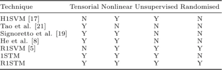
The two closest relevant lines of research to our own work are tensor learning and kernel randomisation, which we briefly review in this section. Table 1 com-pares our work with the most relevant kernel machines.
Tensor learning: To extend SVMs to accept tensorial data input, several studies have focused on re-forming the data representation, e.g., through subspace learning or tensor factorisation. Tao et al. [20] devel-oped supervised tensor learning, a general framework that extends vector-based learning algorithms for use with tensor objects, by applying a combination of con-vex optimisation and multilinear operators. Later in [21], Tao et al. applied their framework to various clas-sical SVM algorithms such asC−SVM [4] andν−SVM
Table 1: Comparison of existing kernel machines with 1STM and R1STM.
Technique Tensorial Nonlinear Unsupervised Randomised
H1SVM [17] N Y Y N Tao et al. [21] Y N N N Signoretto et al. [19] Y Y N N He et al. [8] Y Y N N R1SVM [5] N Y Y Y 1STM Y Y Y N R1STM Y Y Y Y
[18]. In a similar fashion, Cai et al. [3], and Wang and Chen [23] presented a support tensor machine for second-order tensors. Liu et al. [11] introduced a lo-cally maximum margin technique for image and video classification. The key problem with [21, 3, 23, 11] is that they involve an iterative optimisation procedure, raising the problem of non-convex optimisation. Hao et al. [7] overcome this issue by reformulating the linear C−SVM model and obtained a tensor space model.
Note that all the above STMs are restricted to linear classifiers in tensor space. Most recently, [19, 8] have extended the concept of supervised tensor learning into tensor factorisations, to merge the desirable properties of kernel methods and tensor factorisations, for tensorial data that exists on a nonlinear manifold. A common approach to exploit the tensor structure with nonlinear kernel models is to use unfolded matrices to construct nonlinear kernels [19]. However, such methods only capture the relationships within each single mode of the tensor data, because the structural information about inter-mode relationships of tensor data is lost in the unfolding process. To avoid this, He et al. [8] proposed a tensor kernel that preserves tensor structures based on a dual-tensorial mapping, i.e., by mapping each tensor sample from the input space to a higher-order tensor feature space while preserving the structure.
Kernel randomisation: While numerous 1SVM formulations using nonlinear kernels have been proposed in the literature, a common feature of many formula-tions is the solution of a quadratic programming (QP) problem. In particular, these kernel-based methods rely on the computation of a kernel matrix over all pairs of data points, which limits the scalability of training 1SVMs on large datasets. This can also limit the effec-tiveness of 1SVMs on high dimensional inputs, given the need to have sufficiently large training samples spanning the variation in the high dimensional space.
Existing approaches to address the scalability prob-lems of SVMs either preprocess the data prior to build-ing the SVM, e.g., usbuild-ing dimensionality reduction tech-niques such as PCA or Kernel-PCA, or alleviate the QP problem of kernel machines, e.g., by breaking the prob-lem into smaller pieces, for example by using chunking
[22], or sequential minimal optimisation [14]. A more re-cent trend explores the use of randomisation, such as lin-ear random projection [2] as a substitute for the compu-tationally expensive cost of kernel matrix construction. An early example is the work of Achlioptas et al. [1], which replaces the kernel function by a randomised ker-nel to speed-up KPCA. The work of Rahimi and Recht [15, 16] made a breakthrough in this approach. They replicated an RBF kernel by randomly projecting the data to a lower dimensional space and then used linear algorithms. Random projection avoids the complexity of traditional optimisation methods needed for nonlin-ear kernels. Recently randomisation has been applied to other kernel machines, such as dot-product kernels [9], polynomial kernels [6], and 1SVM [5].
Inspired by the idea of [8] and [15], in Section 4 we propose a model for using randomised projection in the context of unsupervised tensor learning, and propose a randomised tensorial kernel.
3 Preliminaries
3.1 Notation Throughout this paper vectors are de-noted by bold, italic lower-case letters, e.g.,x, matrices by bold, upright capital letters, e.g.,X, and tensors by calligraphic letters, e.g.,X. Their elements are denoted by indices ranging from 1 to the capital letter of the index, e.g., n= 1, . . . N. X ∈ RI1×,...,×IN means X is a real Nth-order tensor. R denotes the rank of tensor.
k.kF denotes the Frobenius norm.
3.2 Tensor Algebra
Definition 3.1. (Tensor) An Nth−order tensor
X ∈ RI1×...×IN is a multi dimensional array of real
numbers. An elment ofX is denoted byxi1,...,iN, where 16in6In, and16n6N.
Definition 3.2. (Tensor Product) The tensor
product, also known as outer product, of two tensors
X ∈RI1×...×IN andY ∈ RI 0 1×...×I 0 M is defined by (3.1)
(X ⊗ Y)i1,...,iN,i01,...,i0M =xi1,...,iNyi
0
1, . . . , i0M for all values of the indices.
Definition 3.3. (Inner Product) The inner
prod-uct, also known as scaler prodprod-uct, of two same size ten-sorsX,Y ∈RI1×...×IN is defined as the sum of the prod-ucts of their entries:
hX,Yi= I1 X i1=1 . . . IN X iN=1 xi1,...,iNyi1,...,iN. (3.2)
Definition 3.4. (Frobenius Norm) The Frobenius
norm of a tensor X ∈ RI1×...×IN computes the square
root of the sum of the squares of all its elements, (3.3) kX kF = p hX,X i= v u u t I1 X i1=1 . . . IN X iN=1 x2 i1,...,iN.
Definition 3.5. (Rank-1 Tensor) An Nth−order
tensor X has rank one if it is the tensor product of N vectors ui∈RIi, where16i6N, X =u1⊗. . .⊗uN = N Y n=1 ⊗un. (3.4) The rank R of an Nth
−order tensor X is determined by the minimum number of rank-1 tensors that produce
X in a linear combination.
Definition 3.6. (CP Factorisation) Given a
ten-sor X ∈ RI1×...×IN, it can be factorised if it can be
decomposed as rank-one tensors with length R,
X = R X r=1 x(1)r ⊗. . .⊗x(rN). (3.5) 3.3 One-class SVM (1SVM) Let X = {xi : i = 1, . . . , M} be a set of training samples and yi ∈
{−1,1} be their corresponding labels. In practice,
X is mapped from the input space Rn to a feature
space RH via a nonlinear function φ(.) : R → RH,
resulting in a set of image vectors Xφ = {φ(xi) : i = 1, . . . , M}. A hyperplane-based 1SVM (H1SVM) [17] aims to identify anomalies in the feature space by finding the hyperplane that best separates the data from the origin. The decision function of H1SVM returns +1 in a region where most of the data points occur (i.e., where the probability density is high), and returns
−1 elsewhere. This problem can be formulated as the following quadratic optimisation function:
min w,ξ, ρ 1 2kwk 2+ 1 M ν M X i=1 ξi−ρ (3.6) s.t. (w.φ(xi))≥ρ−ξi, ξi≥0, ∀i= 1, . . . , M.
where ν ∈ (0,1] is a regularisation parameter that controls the fraction of anomalies and the fraction of support vectors, and ξi are the slack variables that allow some of the data vectors to lie on the wrong side of the hyperplane. Since non-zero slack variables ξi are penalised in the objective function, the H1SVM
estimates a decision function f(x) = sgn(w.φ(x)−ρ) that maximises the distance of all the data points (in the feature space) from the hyperplane to the origin, parameterised by a weight vectorw and an offsetρ.
By introducing the Lagrange multipliers and setting the primal variables w, ξ and ρ equal to zero, the quadratic program can be derived as the dual of the primal program in Eq. (3.6):
min α 1 2 P ijαiαjk(xi,xj) (3.7) s.t. 0≤αi ≤M ν1 , P iαi= 1,
where αi are the Lagrange multipliers. The decision function is defined as:
f(x) = sgn(w.φ(x)−ρ), (3.8) = sgn M X i=1 αik(xi,x)−ρ ! . 4 Our Approach
In this section we first introduce the 1STM and then describe our randomised tensorial kernel.
4.1 One-class Support Tensor Machine (1STM)
Let{Xi, yi}be a pair corresponding to a training sample for binary classification, where Xi ∈ RI1×,...,×IN is an
Nth-order tensor andyi
∈ {−1,1}is the corresponding label for i = 1, . . . , M. In [8] it was shown that the tensor binary classification problem can be modeled as a convex quadratic optimization problem in the framework of the standard nonlinear SVM. Based on this finding and the H1SVM, we present a framework for a one-class STM.
The optimization problem of binary tensor classifi-cation can be formulated as follows:
min W,b,ξ 1 2kWk 2 F+C M X i=1 ξi, (4.9) s.t. yi(hW, φ(Xi)i+b)≥1−ξi, ξi≥0,∀i= 1, . . . , M,
where W is the weight tensor of the separating hyper-plane, C is a regularisation parameter that balances the trade-off between the classification margin and misclassification error, and b is the bias. Let φ be a feature mapping that maps a dataset into the Hilbert spaceH, given a tensorX ∈RI1×,...,IN then
φ:X →φ(X)∈RH1×...×Hq.
(4.10)
The optimisation problem in Eq. (4.9) is a gener-alisation of the standard nonlinear SVM. The mapping
function projects each mode ofX to a higher dimension called the high-dimensional tensor space. To perform anomaly detection one needs to find the hyperplane that best separates the data from the origin. In other words, the decision function in the 1STM returns +1 in the re-gion where most of the data points occur, and returns -1 elsewhere. To separate the data set from the origin, we solve the following quadratic program:
min W,ξ,ρ 1 2kWk 2 F+ 1 M ν M X i=1 ξi−ρ (4.11) s.t. (hW, φ(Xi)i)≥ρ−ξi, ξi ≥0,∀i= 1, . . . , M.
By introducing the Lagrange multipliers, we arrive at the following quadratic problem, which is the dual of the primal problem in Eq. (4.11):
min α1,...,αM 1 2 M X i,j=1 αiαjk(Xi,Xj), (4.12) s.t. 0≤αi≤ M ν1 , M X i=1 αi= 1. Further, W = P
iαiφ(Xi). Using the Karush-Kuhn-Tucker optimality conditions (KKT conditions), tensor data can be characterised in terms of whether they fall below, above, or on the hyperplane boundary in the feature space depending on the correspondingαivalues. Tensor data with positive αi values are the support tensors. Further, for 0 < αi <1/M ν, the tensor data fall on the hyperplane and hence ρ can be recovered using these tensors, given that ρ = hW,φ(Xi)i =
P
jαjk(Xj,Xi). Therefore, the tensor-based decision function can be written as
f(X) = sgn M X i=1 αik(X,Xi)−ρ ! . (4.13)
The solution to the quadratic program in Eq. (4.13) is characterised by the parameterν, which sets an upper bound on the fraction of anomalies (training examples regarded as out-of-class) and a lower bound on the number of training examples used as support vectors.
Like other kernel machines, learning with the 1STM degenerates into computing the kernel function. A ten-sor dataset retains the essential information embedded in its multiway structure, therefore an important as-pect of kernel learning for such complex objects is to represent them by sets of key structural features and design kernels on such sets. CP factorisation extracts a structure-preserving kernel in the tensor product fea-ture space. In this way, each tensor object is represented
as a sum of rank-one tensors in the original space, and is then mapped to the tensor product feature space for tensor kernel learning [8].
Let X = PR r=1 QN n=1⊗X (n) r be the CP factorisa-tion of X ∈RI1×...×IN. When a tensor’s rank R = 1, the feature space tensor mapping is defined as
φ:X(n)
→φ(X(n))
∈RH1×...×HN,
(4.14)
and the kernel for two same-sized tensors X and Y is reduced to k(X,Y) = N Y n=1 k(x(n),y(n)). (4.15)
In the case of higher-order tensors the kernel can be derived in a similar fashion. Given that the tensor feature space is a high-dimensional space of the original space, the same operations are applicable. Hence, tensor data can be factorised in the feature space, similar to the original space. Then the mapping is derived as:
φ: R X r=1 N Y n=1 ⊗X(n) → R X r=1 N Y n=1 ⊗φ(X(n)). (4.16)
This corresponds to mapping tensor data into a higher dimensional tensorial feature space and perform-ing the factorisation in this space. Then the kernel in the higher space is just the standard inner product of the tensor data [8],
k R X r=1 N Y n=1 ⊗x(rn), R X r=1 N Y n=1 ⊗y(rn) ! (4.17) = R X i=1 R X j=1 N Y n=1 kx(in),y(jn).
Using popular kernels such as the Gaussian RBF kernel, the above equation can be formulated as: (4.18) k(X,Y) = R X i=1 R X j=1 exp −σ N X n=1 kx(in),y(jn)k2 ! . However, the computational complexity of 1STM grows quadratically with the number of training sam-ples. A linear kernel imposes linear computational com-plexity, but it introduces a bias to the origin. This prob-lem can be removed by using an RBF kernel, which has a higher computational complexity associated with the higher dimensional kernels, thus making it cumbersome for processing large scale datasets.
In order to overcome this limitation, in the next subsection, we propose to exploit nonlinear random projections inside a linear 1STM, which serves as a good approximation of a nonlinear kernel.
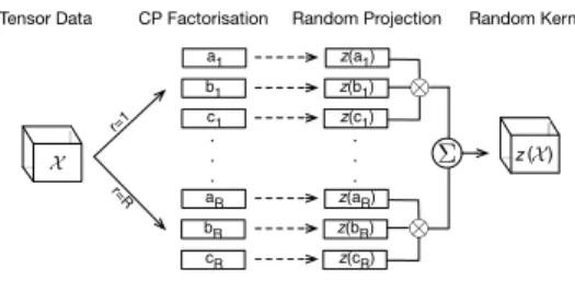
⌦ ⌦ . . . . . . bR cR aR b1 c1 a1 z(bR) z(cR) z(aR) z(b1) z(c1) z(a1) ( )
Tensor Data CP Factorisation Random Projection Random Kernel
⌃ X
X z
r=1
r=R
Figure 1: Random tensorial kernel.
4.2 Randomised 1STM (R1STM) We propose
R1STM, a nonlinear randomised variant of our 1STM, which applies the original linear 1STM method on a randomised nonlinear projection of the tensor data. We first discuss how to generate the nonlinear random fea-tures from the original data, and then we show how to employ these features to detect anomalies using a linear machine. This approach eliminates the need to deal with large kernel matrices for large datasets, con-sequently reducing the computational complexity while achieving comparable detection accuracy to conven-tional nonlinear machines.
4.2.1 Generating Nonlinear Random Features
Consider the problem of fitting a functionf to the data set {Xi, yi}, where yi values are always set to 1 for the one-class problem. This fitting problem consists of findingf that minimises the following empirical risk (4.19) Rreg[f(X)] =Remp[f(X)] +1
2kf(X)k
2
H
where Remp(.) is the empirical risk and 1 2kf(X)k
2
H is the regulariser. The empirical risk is the average loss and can be written as
(4.20) Remp[(X)]≡ 1 M M X i=1 l(f(Xi), yi),
wherel(f(Xi), yi) is the loss function that penalises the deviation between the prediction f(.) and the label y, i.e., this captures the cost of the errors caused whenf(.) is negative on the training samples.
For the 1STM problem, the loss functionl(y, y0) is
of the form l(y, y0) =max(0,1
−yy0). Using the kernel function, the function f(X) = sgn(hW,φ(X)i −ρ) be-comes f(X) =PM
i=1αik(X,Xi). By jointly optimising
over W and αi in a greedy manner, the solution can be found. However, this is computationally intensive. It was proven in [16] that the nonlinear optimisation problem over (α,w1, . . . ,wM) for matrix (and vector) spaces, can be solved by randomly sampling thewi∈Rd
from a data-independent distribution p(w) and creat-ing d-dimensional random features z(X) = [z1· · ·zd],
where zi = [cos(wTi x1+bi), . . . ,cos(wTixM +bi)] and
ej= [cos(wTjy1+bj), . . . ,cos(wTjyM +bj)] are Fourier based random features.
In order to take advantage of this randomisation in our tensorial kernel, we use CP factorisation and randomise the rank-one tensors, as shown in Figure 1. Therefore, Eq. (4.17) is simplified to
k R X r=1 N Y n=1 ⊗x(rn), R X r=1 N Y n=1 ⊗y(rn) ! (4.21) = R X i=1 R X j=1 N Y n=1 (z(in))Te(n) j .
Then, we arrive at the following simplified optimisation problem: min α1∈Rd 1 M P il(α Tz i, yi) (4.22) s.t. kαk∞6B
whereB is a regularisation constant. Furthermore, it is shown by [16] that using randomly selected features in nonlinear spaces causes onlyboundederror compared to using optimised features:
Theorem 4.1. Let p be a
distribu-tion on Ω and |φ(x;w)| 6 1. Let
F =
f(x) =R
δα(w)φ(x;w)dw: |α(w)|6Bp(w) . Draw w1,· · ·,wd iid from p. Further let λ > 0, and l be some L-Lipschitz loss function, then the function f∗(x) =Pd
i=1αiφ(x;wi)minimises the empirical risk
l(f∗(x), y)has a distance from the l-optimal estimator
in F bounded by:
Ep[l(f∗(x), y)]−min
f∈FEp[l(f(x), y)] (4.23) 6O LB √ M + 1 √ dLB r log1 δ !
with a probability of at least1−2δ.
The convergence rate of our randomised R1STM to its original kernel 1STM version can be expressed by the following theorem [12]:
Theorem 4.2. Given the data X ∈ RM×d, a shift
invariant kernelk, a kernel matrixKij =k(xi,xj)and its approximationKˆ usingdrandom features, it can be proven that (4.24) EkKˆ −Kk6 r 3M2logM d + 2MlogM d .
The proof to this theorem can be found in [12].
Mode 3 Mode1 Mode2 00.10.20.30.40.50.60.70.80.91 0 0.1 0.2 0.3 0.4 0.5 0.6 0.7 0.8 0.9 1 00.10.20.30.40.50.60.70.80.91 0 0.1 0.2 0.3 0.4 0.5 0.6 0.7 0.8 0.9 1 Mode 3 Mode 1 Mode 2 00.10.20.30.40.50.60.70.80.91 0 0.1 0.2 0.3 0.4 0.5 0.6 0.7 0.8 0.9 1 00.10.20.30.40.50.60.70.80.91 0 0.1 0.2 0.3 0.4 0.5 0.6 0.7 0.8 0.9 1
Figure 2: Illustration of third-order CASIAA and Banana datasets.
5 Empirical Analysis
In this section, we evaluate the performance of our 1STM and R1STM techniques with experiments on eight real dataset and two synthetic datasets. The aim of these experiments is to compare the performance of the proposed techniques in terms of accuracy and effi-ciency with conventional anomaly detection approaches.
Datasets: The experiments are conducted on four sensor measurement datasets1 that are formed
into third-order tensors (i.e., features×samples×time): (i) Daily and Sport Activity (DSA), (ii) Gas Sen-sor Arrays in Open Sampling Settings (GSAOS)2,
(iii) PAMAP2 Physical Activity Monitoring Dataset (PAMAP2), and (iv) University of Southern Califor-nia Human Activity Dataset (UHAD); and four gait datasets (v) University of South Florida Gait (USFG) including 3 gait recognition datasets with 32, 64 and 128 number of features, and (vi) dataset A from CASIA gait recognition3(CASIAA). We also use a synthetic dataset
known as (vii) Banana dataset, which is a mixture of two banana shaped distributions. The components of these two datasets are randomly moved in any two modes. Table 2 summarises more details about these datasets, and Figure 2 shows two examples of tensorial represen-tations of the CASIAA and Banana datasets.
Baseline methods: To evaluate the performance and efficiency of 1STM and R1STM, we compare them with the following unsupervised baseline methods:
(i) H1SVM [17]: a hyperplaned based 1SVM with RBF kernel, one of the most prevalent anomaly detec-tion techniques.
(ii) R1SVM (Randomised 1SVM) [5]: our work on 1SVMs with randomised kernels, replacing nonlinear kernels with random features and a linear classifier.
(iii) DRDAE (Deep Recurrent Denoising Autoen-coder) [13]: a recurrent implementation of a state-of-the-art deep learning technique known as a Denoising Autoencoder. Since all of the datasets are time series, it is interesting to compare our approaches with an
ef-1Datasets i–iii are from the UCI repository, and dataset iv is from http://sipi.usc.edu/HAD/.
2The original GSAOS dataset contains about 2 million fea-tures, but in this study only the first 13800 features were used.
Table 2: Details of datasets.
Dataset Banana DSA GSAOS PAMAP2 UHAD USFG32 USFG64 USFG3128 CASIAA Features 80×80×20 125×45×60 150×92×50 52×100×50 6×600×5 32×22×10 64×44×20 128×88×20 240×352×15
Objects 500 152 360 344 168 731 731 731 1162
Table 3: Comparison of AUC, training and test time (in seconds) of 1STM and R1STM with conventional anomaly detection techniques.
H1SV M DRDAE R1SV M 1ST M R1ST M
Dataset AUC Train Test AUC Train Test AUC Train Test AUC Train Test AUC Train Test Banana 0.78 4.77×10⁵ 6.65×10³ 0.98 7.69×10² 96.48 0.98 3.21 1.16 0.93 12.43 4.35 0.98 2.11 0.91 DSA 0.84 8.04×10³ 6.73×10² 0.98 6.15×10² 8.12 0.98 0.56 0.06 0.98 0.27 0.13 0.99 0.09 0.04 GSAOS 0.83 1.70×10³ 6.01×10² 0.98 3.49×10² 10.09 0.99 0.21 0.03 0.96 0.45 0.22 0.99 0.05 0.02 PAMAP2 0.90 2.07×10⁵ 6.23×10³ 0.96 4.87×10² 52.02 0.96 1.38 0.29 0.97 2.72 1.43 0.98 0.51 0.24 UHAD 0.85 2.97×10⁴ 1.56×10³ 0.96 2.05×10² 21.19 0.96 0.10 0.02 0.95 0.41 0.20 0.99 0.14 0.07 USFG32 0.86 2.23×10⁵ 4.33×10³ 0.97 4.83×10² 61.00 0.96 1.62 0.68 0.93 7.32 2.92 0.99 1.36 0.58 USFG64 0.87 2.94×10⁵ 4.86×10³ 0.97 5.08×10² 69.41 0.97 1.69 0.74 0.94 8.01 3.46 0.99 1.52 0.71 USFG128 0.88 4.18×10⁵ 5.37×10³ 0.97 5.63×10² 87.32 0.97 1.83 0.85 0.96 8.12 3.94 0.99 1.71 0.80 CASIAA 0.81 5.32×10⁵ 7.75×10³ 0.98 1.21×10³ 1.35×10² 0.96 6.06 2.16 0.95 18.21 5.14 0.98 3.01 1.12 Average 0.86 2.32×10⁵ 3.57×10³ 0.97 5.76×10³ 60.10 0.97 1.85 0.67 0.95 6.44 2.42 0.99 1.14 0.50
fective sequential data modeling technique, which com-bines the multiple levels of representation.
Experimental setup: All the records in each dataset are normalised between [0,1], and mixed with 5% anomalous objects, randomly drawn from U(0,1).
All the hyper-parameters in our learning models, com-prising the width ν (0−1) and gamma g (−4−4) for H1SVM, the learning rate (0.001−0.1), number of epochs (10−200), and number of hidden units (hn) for the autoencoder, and the rankR(1−12) for CP fac-torisation [7, 8], are selected through grid search based on the best performance on a validation set. Note that training is performed in an unsupervised way, and labels are only used for testing.
Metrics: The Receiver Operating Characteristic (ROC) curve and the corresponding Area Under the Curve (AUC) are used to measure the accuracy of all the methods. The reported training/testing times are in seconds based on experiments run on a machine with an Intel(R) Core(TM) i7 CPU at 3.60 GHz and 16 GB RAM. For 1SVM based methods LIBSVM was used.
5.1 Performance Evaluation Table 3 shows the performance results and their average over all the datasets. The best case, i.e., the highest AUC and lowest training/test time, for each dataset is stressed through bold-face. The reported time only includes the training and test time of the studied models, and no preprocessing time, e.g., data vectorisation or fac-torisation, has been included. Section 5.3 analyses the preprocessing stage of 1STM and R1STM. For ease of interpreting the reported results, Figure 3 graphically demonstrates the average rankings of the three metrics, AUC, training and test time, obtained from Friedman’s test. As shown in this graph, R1STM delivers the best
Table 4: Wilcoxon test to compare the performance of the studied methods regarding thep-values. W+ corresponds to the sum of the ranks for the method on the left, and W−for the right.
The W values in bold indicate that the null hypothesis is rejected for the corresponding method.
Accuracy Training Time Test Time Method W+W− p W+W− p W+W− p R1STM vs. 1STM 45 0 0.0039 0 45 0.0039 0 45 0.0039 R1STM vs. R1SVM 28 1 0.0156 1 44 0.0078 5 40 0.0391 R1STM vs. DRDAE 28 0 0.0156 0 45 0.0039 0 45 0.0039 R1STM vs. 1SVM 45 0 0.0039 0 45 0.0039 0 45 0.0039 1STM vs. R1SVM 2.5 33.50.0391 43 2 0.0117 45 0 0.0039 1STM vs. DRDAE 2 26 0.0313 0 45 0.0039 0 45 0.0039 1STM vs. 1SVM 36 0 0.0078 0 45 0.0039 0 45 0.0039 R1SVM vs. DRDAE 1.5 4.5 0.7500 0 45 0.0039 0 45 0.0039 R1SVM vs. 1SVM 45 0 0.0039 0 45 0.0039 0 45 0.0039 DRDAE vs. 1SVM 45 0 0.0039 0 45 0.0039 0 45 0.0039
performance both in terms of accuracy and efficiency. A statistical analysis is performed to explore the ef-fect of tensor representation and randomisation on these results, and also to assess the statistical significance of the performance of the various methods. For this pur-pose, we perform pairwise comparisons between differ-ent methods using the Wilcoxon signed-rank test. The test returns ap-value associated with each comparison, representing the lowest level of significance of a hypoth-esis that results in a rejection. This value allows one to determine whether two algorithms have significantly different performance and to what extent. For all the comparisons in this study the significance levelαis set to 0.05. Table 4 summarises the output of this compar-ison on all the performance results from Table 3.
Comparing 1STM with H1SVM, a significant boost is obtained in both accuracy and efficiency revealing the beneficial effect of the tensorial representation. Similar results are achieved when using randomisation, i.e., R1SVM vs. H1SVM, but the best result occurs
H1SVM DRDAE R1SVM 1STM R1STM 1 2 3 4 5 Average Rank 5 2.5 2.5 4 1 5 4 2 3 1 5 4 3 2 1 AUC Train time Test time
Figure 3: Comparison of rankings of anomaly detection methods for 3 metrics. The bars represent average rankings based on the Friedman test, and the number on the top of the bars indicates the ranking of the algorithm, from the best (1) to worst (5) for each given measure, and if a tie occurs then the best mean result is taken. The ranking is determined for all datasets and finally an average is calculated as the mean of all rankings.
Percentage of shuffled objects
0 5 10 15 20 25 30 Accuracy 0.75 0.8 0.85 0.9 0.95 1 Banana UHAD CASSIA Banana UHAD CASSIA
Figure 4: Comparison of accuracy with respect to increasing the percentage of shuffled objects. The solid and lines present the results for 1STM and the dotted lines present for R1STM.
when using the tensorial representation in conjunction with randomisation. The p−values in the comparison of R1STM with 1STM and R1SVM, reject the null hypothesis for the accuracy and efficiency measures with a level of significance ofα= 0.05, implying a significant improvement of R1STM over the two other methods.
5.2 Effect of Tensorial Representation The main objective of the tensor representation of data is to retain the natural structure and correlation of the records. To study this effect on 1STM and R1STM, we shuffled the third order (sequence) of some of the test objects in the Banana, UHAD and CASIAA datasets. As shown in Figure 4, the accuracy of the tensor machines decreases as the percentage of the shuffled objects increases.
That is, existing techniques have a fatal modelling flaw in that they fail to capture the inherent sequential nature of data and treat the inputs as bags of randomly permutable items agnostic to any sequential structure. This modelling property essentially suggests that the test objects could be randomly shuffled and still result in the same object. To overcome this limitation, a tensor representation is proposed to faithfully represent the spatio-temporal dependencies in the data.
5.3 Rank Sensitivity Evaluation The optimal rank R of CP factorisation is conventionally found through grid search, but it is important to determine the sensitivity of this parameter in training 1STM and
Rank 1 2 3 4 5 6 7 8 Accuracy 0.7 0.8 0.9 1 Banana DSA GSAOS PAMAP2 UHAD Rank 1 2 3 4 5 6 7 8 Accuracy 0.7 0.8 0.9 1 USFG32 USFG64 USFG128 CASIAA
Figure 5: Comparison of accuracy with respect to increasing number of CP ranksR.
Percentage of data
60 70 80 90 100
Time (in seconds)
0 5 10 15 20 Train 1STM R1STM 1STM R1STM Percentage of data 60 70 80 90 100
Time (in seconds)
0 1 2 3 4 5 6 Test 1STM R1STM 1STM R1STM
Figure 6: Comparison of accuracy with respect to increasing the percentage of sample objects. The solid dotted lines present the results for USF128 and CASIAA dataset, respectively.
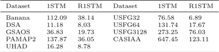
R1STM. Deliberate adjustment of Ris important since it plays a significant role in the performance of the al-gorithms. Moreover, a higher value of R indicates a higher number of items, and correspondingly a higher training/test time of the model. Figure 5 shows the re-sults of our experiments conducted on all the datasets to measure the sensitivity of 1STM to R. As can be seen in this figure, the optimal value of R for 1STM is quite data dependent, it varies from one to the other. In this experiment, the range of R ∈ [1,12] were con-sidered, but since no improvement was observed for val-ues larger than 8, only the results from the range of R ∈ [1,8] were reported. In the range of R ∈ [1,2], R1STM delivers the AUC values presented in Table 3. For higher values ofR, the AUC value slightly fluctuates (about 1%), hence no figure was included for R1STM. Table 5 compares the factorisation time of 1STM and R1STM. From this experiment it can be concluded that although CP factorisation adds an extra parameter to the list of grid-search, the optimal value of R lies in a narrow range, especially in the case of R1STM.
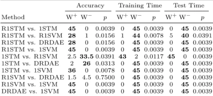
5.4 Scalability Evaluation A desirable property of an anomaly detection method, in addition to accu-racy, is its efficiency and scalability. The computa-tional and memory complexity of 1STM and R1STM areO(DM2R2) andO(dM R), respectively, whereD=
QN
n=1In, d =
QN
n=1Jn, and Jn In. The
scalabil-ity comparison of these two algorithms on two largest datasets, CASIAA and USF128, suggests that the train-ing/testing time of the randomised methods, unlike
Table 5: Comparison of CP decomposition time (in seconds) for 1STM and R1STM. Dataset 1STM R1STM Dataset 1STM R1STM Banana 112.09 38.14 USFG32 76.58 6.89 DSA 11.18 8.03 USFG64 131.74 17.67 GSAOS 36.83 19.73 USFG3128 273.25 76.03 PAMAP2 137.87 36.05 CASIAA 647.45 123.11 UHAD 16.28 8.78
1STM, grow linearly at a fairly low rate, see Figure 6.
6 Conclusions and Future Work
In this paper we have introduced two unsupervised ten-sorial anomaly detection methods, 1STM and R1STM, that directly apply to tensor objects and retain the data’s structure. 1STM is an extension of the conven-tional one-class SVMs to tensor space. R1STM, ad-ditionally, approximates the nonlinear tensorial kernel through applying the original linear classifier method on a randomised nonlinear projection of the data. Our empirical analysis on several benchmark and synthetic datasets shows that 1STM and R1STM not only main-tain the data’s structure, but also they deliver signifi-cant improvements over conventional anomaly detection methods — especially R1STM, which achieves better or comparable performance to a state-of-the-art deep recurrent autoencoder, while reducing its training and testing time by more than two orders of magnitude.
References
[1] Dimitris Achlioptas, Frank McSherry, and Bernhard Sch¨olkopf. Sampling techniques for kernel methods. InAdvances in Neural Information Processing Systems (NIPS), 2002.
[2] Avrim Blum. Random projection, margins, kernels, and feature-selection. In Subspace, Latent Structure and Feature Selection, pages 52–68. 2006.
[3] Deng Cai, Xiaofei He, Ji-Rong Wen, Jiawei Han, and Wei-Ying Ma. Support tensor machines for text cate-gorization. Technical Report 2714, University of Illinois at Urbana-Champaign, 2006.
[4] Corinna Cortes and Vladimir Vapnik. Support-vector networks. Machine Learning, 20(3):273–297, 1995. [5] Sarah M. Erfani, Mahsa Baktashmotlagh, Sutharshan
Rajasegarar, Shanika Karunasekera, and Chris Leckie. R1SVM: a randomised nonlinear approach to large-scale anomaly detection. InTwenty-Ninth Conference on Artificial Intelligence (AAAI), 2015.
[6] Raffay Hamid, Ying Xiao, Alex Gittens, and Dennis DeCoste. Compact random feature maps. In Interna-tional Conference on Machine Learning (ICML), 2014. [7] Zhifeng Hao, Lifang He, Bingqian Chen, and Xiaowei Yang. A linear support higher-order tensor machine for
classification. IEEE Transactions on Image Processing, 22(7):2911–2920, 2013.
[8] Lifang He, Xiangnan Kong, S Yu Philip, Ann B Ra-gin, Zhifeng Hao, and Xiaowei Yang. Dusk: A dual structure-preserving kernel for supervised tensor learn-ing with applications to neuroimages. InSIAM Inter-national Conference on Data Mining (SDM), 2014. [9] Purushottam Kar and Harish Karnick. Random feature
maps for dot product kernels. In International Con-ference on Artificial Intelligence and Statistics (AIS-TATS), 2012.
[10] Tamara G Kolda and Brett W Bader. Tensor decompo-sitions and applications. SIAM Review, 51(3):455–500, 2009.
[11] Yang Liu, Yan Liu, and Keith CC Chan. Tensor-based locally maximum margin classifier for image and video classification. Computer Vision and Image Understanding, 115(3):300–309, 2011.
[12] David Lopez-Paz, Suvrit Sra, Alex Smola, Zoubin Ghahramani, and Bernhard Sch¨olkopf. Randomized nonlinear component analysis. In International Con-ference on Machine Learning (ICML), 2014.
[13] Andrew L Maas, Quoc V Le, Tyler M O’Neil, Oriol Vinyals, Patrick Nguyen, and Andrew Y Ng. Recurrent neural networks for noise reduction in robust ASR. In INTERSPEECH, 2012.
[14] John C Platt. Fast training of support vector machines using sequential minimal optimization. InAdvances in Kernel Methods, pages 185–208, 1999.
[15] Ali Rahimi and Benjamin Recht. Random features for large-scale kernel machines. InAdvances in Neural Information Processing Systems (NIPS), 2007. [16] Ali Rahimi and Benjamin Recht. Weighted sums of
random kitchen sinks: Replacing minimization with randomization in learning. In Advances in Neural Information Processing Systems (NIPS), 2009. [17] Bernhard Sch¨olkopf, John C Platt, John Shawe-Taylor,
Alex J Smola, and Robert C Williamson. Estimating the support of a high-dimensional distribution. Neural Computation, 13(7):1443–1471, 2001.
[18] Bernhard Sch¨olkopf, Alex J Smola, Robert C Williamson, and Peter L Bartlett. New support vec-tor algorithms. Neural Computation, 12(5):1207–1245, 2000.
[19] Marco Signoretto, Lieven De Lathauwer, and Johan AK Suykens. A kernel-based framework to tensorial data analysis. Neural Networks, 24(8):861–874, 2011. [20] Dacheng Tao, Xuelong Li, Weiming Hu, Stephen
May-bank, and Xindong Wu. Supervised tensor learning. In IEEE International Conference on Data Mining, 2005. [21] Dacheng Tao, Xuelong Li, Xindong Wu, Weiming Hu, and Stephen J Maybank. Supervised tensor learning. Knowledge & Information Systems, 13(1), 2007. [22] Vladimir Naumovich Vapnik and Vlamimir Vapnik.
Statistical Learning Theory. Wiley New York, 1998. [23] Zhe Wang and Songcan Chen. New least squares
support vector machines based on matrix patterns. Neural Processing Letters, 26(1):41–56, 2007.