CIRJE Discussion Papers can be downloaded without charge from: http://www.e.u-tokyo.ac.jp/cirje/research/03research02dp.html
Discussion Papers are a series of manuscripts in their draft form. They are not intended for circulation or distribution except as indicated by the author. For that reason Discussion Papers may not be reproduced or distributed without the written consent of the author.
CIRJE-F-567
A New Scheme for Static Hedging of European
Derivatives under Stochastic Volatility Models
Akihiko Takahashi University of Tokyo
Akira Yamazaki
Mizuho-DL Financial Technology Co., Ltd. June 2008
A New Scheme for Static Hedging of European
Derivatives under Stochastic Volatility Models
∗
Akihiko Takahashi and Akira Yamazaki
June 9 2008
Abstract
This paper proposes a new scheme for static hedging of European path-independent derivatives under stochastic volatility models.
First, we show that pricing European path-independent derivatives under stochastic volatility models is transformed to pricing those under one-factor local volatility models.
Next, applying an efficient static replication method for one-dimensional price processes developed by Takahashi and Yamazaki[2007], we present a static hedging scheme for European path-independent derivatives.
Finally, a numerical example comparing our method with a dynamic hedging method under the Heston[1993]’s stochastic volatility model is used to demonstrate that our hedging scheme is effective in practice. Keywords: Static Hedging, Stochastic Volatility, Markovian Projec-tion, Plain Vanilla OpProjec-tion, Heston Model
∗Forthcoming in Journal of Futures Markets.
1
Introduction
This paper develops a new scheme for the static hedging of European path-independent derivatives under stochastic volatility models. When the dynamics of the underlying asset price is described by a multi-dimensional process, a one-dimensional price process that has the same distribution as the original one can be obtained by using the result proved by Gy¨ongy[1986](theorem 4.6 in his paper). Piterbarg[2006] called this resultMarkovian projectionin the context of financial mathematics, and noted that Dupire[1994], Derman and Kani[1998], and Savine[2001] derived essentially the same result in finance. In particular, Savine[2001] applied Tanaka’s formula for the derivation.
Preceding literatures such as Avellaneda, Boyer-Olson, Busca and Friz[2002], Henry-Labordere[2005], Antonov and Misirpashaev[2006], Piterbarg [2006], and Madan, Qian and Ren[2007] used the Gy¨ongy’s theorem mainly for pricing and calibration in some complicated multi-factor models. Due to his theorem, certain approximation formulas of European derivative prices and/or the Black-Scholes equivalent volatilities can be obtained under the models for which it is difficult to derive exact closed-form formulas.
Unlike these literatures, we propose a new application of Gy¨ongy’s theorem in finance, that is a static hedging strategy under stochastic volatility models. Specifically, based on his theorem pricing European path-independent deriva-tives under stochastic volatility models is transformed to pricing those under one-factor local volatility models. Thus, we can apply an efficient method for one-dimensional price processes developed by Takahashi and Yamazaki[2007] to forming a static hedging portfolio for a European derivative: compared with a standard static replication approach, their method of gamma-weighted portfo-lio of options is more efficient, that is, a more precise hedge is derived from a smaller number of options.
In particular, if the drift and diffusion terms of the one-dimensional price processes are obtained analytically, it is easy to implement this scheme. For instance, when the option price is analytically or semi-analytically obtained, the scheme is implemented through the relation between the option price and its volatility function developed by Dupire[1994]. As an example, we derive the
local volatility model that corresponds to the Heston[1993]’s model.
To demonstrate how our scheme works, this paper uses a standard plain vanilla option under the Heston[1993]’s model in a numerical example. It should also be noted that this method can be applied to other European derivatives such as cash digital, asset digital and power options. Finally, simulation ex-ercises comparing our scheme with a dynamic hedging method, specificallythe minimum-variance hedging method(see Bakshi,Cao and Chen[1997] for example) are used to demonstrate that our hedging scheme is effective in practice.
For over a decade, static hedging techniques have been developed and in-vestigated extensively for barrier type options. See, for example, Derman, Er-gener and Kani[1995], Carr, Ellis and Gupta[1998], Carr and Picron[1999] and Fink[2003]. Carr and Chou[1997] shows the representation of any twice differ-entiable payoff functions, that is the basis for theorem 2 in this paper as well as for proposition 1 of Takahashi and Yamazaki[2007]. Their paper then devel-ops the so calledstrike-spreads method for static hedging of barrier under the Black-Scholes model.
More recently, Carr and Lee[2008] extends put-call symmetry(PCS) and ap-plies it to constructing semi-static replications for barrier-type claims under general asset dynamics. For other works related with static hedging of barrier options, see their paper and references therein.
On the other hand, Carr and Wu[2002] concentrates on an efficient replica-tion of a plain vanilla opreplica-tion though their approach implies the possibility of further extensions and applications. It also applies the Gauss-Hermite quadra-ture rule to approximate static hedging of the option by plain vanilla options with shorter terms under the Black-Scholes and Merton[1976] jump-diffusion models. Moreover, their paper undertakes extensive simulation exercises to in-vestigate the robustness of the method. In a certain sense, this paper extends the methodologies developed by Carr and Wu[2002], Carr and Chou[1997] and Carr and Madan[1998, 1999] to stochastic volatility models.
The remainder of the paper is organized as follows. The next section presents our proposed method for static hedging, and also provides a key result for the Heston[1993]’s stochastic volatility model in our framework. Section 3 shows a numerical example and concluding remarks are presented in Section 4.
2
New scheme for static hedging of European
path-independent derivatives
This section presents a new scheme for static hedging of European options. Specifically, under stochastic volatility models, we develop a methodology to hedge European path-independent derivatives and their portfolios based on a
staticportfolio of shorter term plain vanilla options. Staticportfolio implies that the weights in the portfolio remain unchanged when the prices of underlying assets move and options in the portfolio approach maturity. This static hedging scheme is not entirely perfect, but provides much better performance than a dynamic hedging method. Robustness of our scheme will be shown in section 3. Under the assumptions of a frictionless and no-arbitrage market, let St de-note the spot price of a stock, an underlying asset at timet∈[0, T∗] where T∗
is some arbitrarily fixed time horizon. For sake of simplicity, the interest rate
rand the dividend yieldq are assumed to be constants. The no-arbitrage con-dition ensures the existence of a risk-neutral probability measureQ such that the instantaneous expected rate of return on every asset is equal to the instan-taneous interest rater. Furthermore, the risk-neutral process of the underlying asset price is assumed to be an Itˆo process under a filtered probability space (Ω,F,{Ft}t∈[0,T∗],Q). In addition, the analysis in this paper concentrates on
static hedging of European path-independent options where the final payoff of the option is solely determined by the stock price at maturity. Typical examples in this class include plain vanilla, cash digital, asset digital and power options.
2.1
General case
Suppose that the underlying asset priceS under the risk-neutral measure Qis evolved by a stochastic volatility model. In particular, (S, V) is a R2++-valued process and it is the unique solution of a stochastic differential equation given (S0, V0)∈R2++:
dSt = cStdt+
√
VtSt¯σ1dWt (1)
wherec:=r−qis a constant andW = (W1, W2) is a 2-dimensional Brownian motion. Here µ andσ2 are R-valued {Ft}-progressively measurable processes that guarantee the unique solution to the stochastic differential equation. Also, ¯
σi(i = 1,2) are defined by ¯σ1 = (1,0) and ¯σ2 = (ρ,
√
1−ρ2)(|ρ| ≤ 1)
respec-tively.
Our subsequent analysis relies on the next result due to Gy¨ongy [1986].
Theorem 1 (Gy¨ongy [1986];theorem 4.6)
ξ is aRn-valued process and it is the unique solution of a stochastic
differ-ential equation: ξt=x0+ ∫ t 0 β(ω, u)du+ ∫ t 0 δ(ω, u)dWu
where x0 ∈ Rn, β and δ are bounded measurable Fu-adapted Rn-valued and
Rn×n-valued processes respectively, and W is a n-dimensional Brownian
mo-tion.
We put a condition:
∑
i,j
αi,jzizj≥p|z|2
for every(ω, t)∈Ω×[0,∞)andz∈Rn whereα:=δδ⊤ andpis a fixed positive
constant. Here,x⊤ denotes the transpose of x.
Under the condition, the stochastic differential equation:
Xt=x0+ ∫ t 0 b(Xu, u)du+ ∫ t 0 σ(Xu, u)dWu
admits a weak solution X¯t which has the same one-dimensional distribution as
ξt, where b: Rn×[0,∞)→Rn andσ:Rn×[0,∞)→Rn×n are respectively
bounded measurable functions such that
b(x, t) := E[β(t)|ξt=x]
σ(x, t) := E[δ(t)δ(t)⊤|ξt=x] 1 2.
For pricing a European path-independent derivative, only the distribution at maturity of the underlying asset price does matter. Hence, due to Gy¨ongy’s above theorem, pricing a European path-independent derivative under the stochas-tic volatility model (1) is transformed to pricing it under a local volatility model ifSis regarded asξin his theorem. This result is stated as the following propo-sition:
Proposition 1 Suppose that fT(S)is the payoff at maturity T of a European
path-independent derivative whose randomness depends solely on the underlying price at maturity, ST. Suppose also that the time-0 price function v0(y, z) of
the derivative under the stochastic volatility model (1) withS0=y andV0=z. then, v0(y, z)is given by:
v0(y, z) =e−rTE[fT( ˆS)],
where E[·] denotes the expectation operator under the risk-neutral probability measureQ, andSˆ follows a local volatility model:
dSˆt=cSˆtdt+σ( ˆSt, t)dW1t; ˆS0=y. (2)
Here,σ(x, t)is defined by:
σ(x, t) :=E[Vt|St=x] 1
2. (3)
Also, in stead of getting the local volatilityσ(x, t) by evaluating the right hand side of (3), we can sometimes obtain it easier through the following Dupire [1994]’s result:
Proposition 2 (Dupire [1994]) Suppose that the underlying spot price Sˆ is evolved by a local volatility model (2). Let C(t, x) := C(y;t, x) represent the time-0 price of a plain vanilla call option with spot price Sˆ0 =y, strike xand
maturityt. Then, the local volatilityσ(x, t)is given by:
σ2(x, t) = 2qC(t, x) +cx ∂ ∂xC(t, x) + ∂ ∂tC(t, x) x2 ∂2 ∂x2C(t, x) . (4)
Note that the option prices and its derivatives appearing in the right hand side of (4) is equivalent to those under the stochastic volatility model (1). Hence, if the option prices and the derivatives under the stochastic volatility model is obtained analytically or semi-analytically, then the local volatility is easy to calculate. We will see this case using the Heston[1993]’s model in the next subsection.
Of course, when pricing derivatives under the stochastic volatility model is possible analytically, the transformation to a local volatility model does not have any advantage in terms of valuation. However, in terms of hedging, it does have advantage because the reduction of a two-factor model to a one-factor model allows us the direct application of proposition 1 in Takahashi and Yamazaki[2007]. The following theorem is our main result.
Theorem 2 Suppose thatfT(S)is the payoff at maturityT of a European
path-independent derivative and that its underlying asset price is evolved by the model (1). Also let τ ∈[0, T] and suppose that the time-τ price functionvˆτ( ˆS)of the
European derivative under model (2) is twice differentiable for all Sˆ ≥0, that is, both the delta and gamma of the derivative exist at timeτ. Here, the process
ˆ
S is the solution to the stochastic differential equation of (2). Then, it holds that for anyκ >0,
v0(y, z) =e−rτˆvτ(κ) +e−rτ∂vˆτ ∂Sˆ |Sˆ=κ{F(τ)−κ} + ∫ κ 0 ∂2ˆv τ ∂Sˆ2 |Sˆ=xP(τ, x)dx+ ∫ +∞ κ ∂2vˆ τ ∂Sˆ2 |Sˆ=xC(τ, x)dx, (5)
where F(τ) denotes the time-0 price of the forward contract with maturity τ, andP(τ, x)andC(τ, x)represent the time-0 prices of plain vanilla put and call options with spot price y, strikexand maturity τ respectively.
The implication of this theorem is that the risk embedded in a target European derivative can be hedged using astaticportfolio of liquid plain vanilla options with a maturity that is shorter than the maturity of the target derivative. The equation (5) implies that the static portfolio consists of the following securities with maturitiesτ; ∂2ˆvτ
∂Sˆ2 |Sˆ=xdxunits of a call with strikexfor eachx > κand ∂2ˆvτ
∂Sˆ2 |Sˆ=x dx units of a put with strike x for each x < κas well as ∂vτˆ
units of a forward contract with delivery priceκand ˆvτ(κ) units of a zero coupon bond with face value 1. Here static portfolio indicates that once the hedging portfolio is created, re-balancing is unnecessary until the maturity date of the options in the portfolio.
Finally, theorem 1 in Takahashi and Yamazaki[2007] provides a practically efficient scheme based on the Gauss-Legendre quadrature rule for approximating the theoretical hedging portfolio given by the right hand side of (5). We will show the validity of our scheme in the next section through a numerical example.
Remark 1 The equation (5) indicates that the value of the target derivative is replicated exactly by the hedging portfolio at time-0. However, after time-0to the end of the hedging period the value may not be replicated for all the realization of(St, Vt)fort∈(0, τ]; more precisely, if the realization ofVtgivenStdeviates
from E[Vt|St], the target derivative is not hedged perfectly. Therefore, we need
to examine the performance of our hedging scheme in further detail. In fact, simulation exercises in the next section show that our static scheme provides much better performance than a dynamic hedging method.
Remark 2 When the hedging target is a plain vanilla call option under non-stochastic volatility environment, our theorem 2 is reduced to theorem 1 in Carr and Wu [2002].
2.2
Example: Heston Model
This subsection derives the formula for the volatility functionσ(x, t) under the Heston[1993]’s model used for a numerical example in the next section. The stochastic volatility model (1) becomes the following in this case:
dSt = cStdt+ √ VtSt¯σ1dWt; S0=y (6) dVt = ξ(η−Vt)dt+θ √ Vt¯σ2dWt; V0=z,
whereξ,η andθ are positive constants such that ξη≥θ2/2. Also, ¯σi(i= 1,2) are defined by ¯σ1= (1,0) and ¯σ2= (ρ,√1−ρ2)(|ρ| ≤1) respectively, andW is
a 2-dimensional Brownian motion. We next present expressions for the call price and its derivatives in the right hand side of (4) based on a slight modification
of Carr and Madan[1999]’s Fourier transform method.
Carr and Madan [1999] introduces a fast Fourier transform method for op-tion pricing. This paper proposes to compute the time value of the opop-tion after subtracting an intrinsic value from the option price in order to avoid the oscil-lation of the integrand in the Fourier inversion. As a result, the option price can be obtained as the time value derived by the Fourier inversion plus the intrinsic value. On the other hand, to compute the partial derivatives of a call option with respect to strikeK, we propose to subtract the Black-Scholes price with appropriate volatility from the option price instead of subtracting the in-trinsic value. This choice is made because the inin-trinsic value of a call option is not differentiable. See also p.363 of Cont and Tankov[2003]. (Note that the Black-Scholes call price is twice differentiable with respect to strikeK.)
In the Heston model, let Xt:= ln{St/S0} −ct and thenϕXt(u), the char-acteristic function ofXtis obtained by:
ϕXt(u) = exp{A(u, t)}B(u, t), where A(u, t) := ξηt(ξ−iρθu) θ2 − (u2+iu)V0 γcoth(γt/2) +ξ−iρθu B(u, t) := { cosh(γt/2) +ξ−iρθu γ sinh(γt/2) }−2ξη/θ2 γ := √θ2(u2+iu) + (ξ−iρθu)2, i=√−1.
For the case of the Black-Scholes model (i.e. Sbs
t =S0ect− 1 2σ 2t+σW 1t), note that ϕXbs
t (u), the characteristic function ofX bs
t := ln{Stbs/S0} −ctis expressed as
ϕXbs
t (u) = exp{−σ
2t(u2+iu)/2}. Then, we have the following proposition. The
proof is easy and is omitted.1
Proposition 3 Under the Heston[1993]’s stochastic volatility model (6), let
C(t, x) the call price at time 0 with strike x and maturity t. Then, C(t, x),
∂C(t,x)
∂x ,
∂2C(t,x) ∂x2 and
∂C(t,x)
∂t in (4) are given as follows:
C(t, x) = S0e −αk 2π ∫ ∞ −∞ e−iukζt(u)du+Cbs(t, x) (7) ∂C(t, x) ∂x = −e−(α+1)k 2π ∫ ∞ −∞ (α+iu)e−iukζt(u)du+ ∂Cbs(t, x) ∂x ∂2C(t, x) ∂x2 = e−(α+2)k 2πS0 ∫ ∞ −∞ (α+iu)(α+iu+ 1)e−iukζt(u)du + ∂ 2Cbs(t, x) ∂x2 ∂C(t, x) ∂t = S0e−αk 2π ∫ ∞ −∞ e−iuk∂ζt(u) ∂t du+ ∂Cbs(t, x) ∂t
whereα >0,k:= ln{x/S0},Cbs(t, x)denotes Black-Scholes call price at time 0 with strikexand maturity t, and
ζt(u) := exp{[c(iu+α+ 1)−r]t}
(iu+α)(iu+α+ 1) {ϕXt(u−iα−i)−ϕXbst (u−iα−i)}.
3
Numerical examples
This section shows the validity of our scheme through numerical examples under the Heston[1993]’s model. The examples are two types of simulation test, which are Monte Carlo simulation and historical simulation.
Note first that the market is incomplete under the stochastic volatility model and that the perfect hedge is not possible by dynamic trading of the underly-ing asset. Specifically, we implement hedgunderly-ing simulations comparunderly-ing the per-formance of our scheme with that ofthe minimum-variance hedging method, a standard method of dynamic hedging in an incomplete market. In the minimum-variance hedging method, the units of the underlying asset to be held at each timetare computed as follows:2
∂Ct ∂St +ρθ St ∂Ct ∂Vt , (8)
whereCtdenotes the time-tprice of a target call option , andρandθare param-eters in (6). Here we observe that volatility risk is partially hedged through the
2For example, see Bakshi,Cao and Chen[1997] for the detail and for a practical application
correlation between the underlying asset’s price and its instantaneous variance. Moreover, based on the equation (8), we re-balance the dynamic portfolio once a day in our simulations.
Let us describe briefly the procedure for implementation of our static hedg-ing scheme. First, we transform the Heston model (6) into a local volatility model (2) by applying (7). Next, in order to obtain a static hedging portfolio in theorem 1 of Takahashi and Yamazaki[2007] that is a practical method for implementing theorem 2 in this paper, we need approximations of the price, the delta and gammas of the target option in theorem 2, in other words ˆvτ(κ),
∂ˆvτ
∂Sˆ |Sˆ=xand ∂2ˆvτ
∂Sˆ2 |Sˆ=xin (5) respectively. Solving the relevant partial differen-tial equation(PDE) numerically by the Crank-Nicholson method provides those approximations.
3.1
Monte Carlo simulation test
In Monte Carlo simulations, we consider two cases: the first case(Case 1) is that the Heston parameters are the same under a risk-neutral measure and under the physical measure except a mean reverting rateη, while the second case(Case 2) is that volatility on the varianceθunder the risk-neutral measure is higher than the one under the physical measure. Under the physical measure, we assume thatShas a drift coefficient of 0.06. These parameters are taken form Carr and Lee[2007]. The initial conditions of our simulations and the Heston parameters for the first and second cases are listed in tables 1 and 2 respectively. For both cases, the hedging period is set to beτ = 0.5 while the maturity of the target option isT= 1.0.
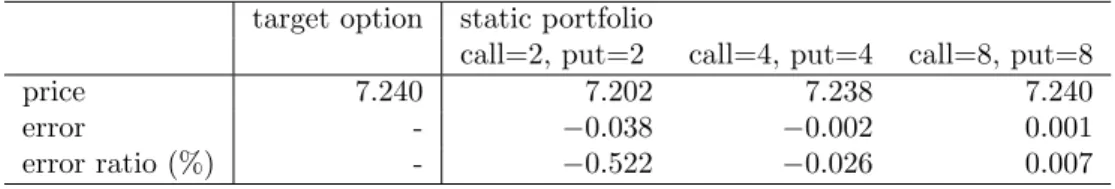
Table 3 shows approximations of the target option’s price by the values of options’ portfolios used for static hedging; the target option’strueprice is given by direct application of Heston[1993]’s formula. Also these static portfolio com-positions are reported in table 4. Clearly, the more the number of options, the better is the approximation. A portfolio of more than eight options gives rather good approximation; the absolute values of the error and the error ratio are less than 0.002 and 0.03% respectively for the portfolio of eight options(call=4, put=4 in the table).
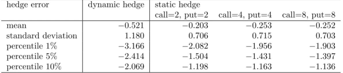
Next, tables 5 and 6 provide basic statistics of Monte Carlo simulation results for Case 1 and Case 2 respectively. Moreover, figure 1 shows the histograms of hedging errors. The statistics and the histograms are based on 10,000 simulated paths. All the statistics and figures shows that our static hedging scheme out-performs the dynamic hedging based onthe minimum-variance hedging method. In particular, for Case 2, that is when the volatility on the variance under the physical measure differs from the one under the risk-neutral measure, our scheme gives more robust result than the dynamic hedging in a sense that its hedging performance is less affected by the parameter’s change than the dy-namic hedging’s performance. Because this situation is common in practice, the result indicates that our static hedging scheme seems useful.
3.2
Historical simulation test
This subsection shows the historical performance of our static hedging scheme in USD/EUR currency option market. The data on USD/EUR currency options are obtained from British Bankers Association’s homepage. They are daily time-series data of plain vanilla options on USD/EUR spot exchange rate from August 2001 to January 2008.
In currency option markets, option prices are provided as Black-Scholes im-plied volatilities and the moneyness of an option is expressed in terms of Black-Scholes delta, rather than its strike price(See Carr and Wu[2005] for the detail). Using the daily data of 25-delta call, 25-delta put and ATM with 3-month and 1-year maturities and re-calibrating the Heston model every business day, we compare the performance of the static hedging with that of the minimum-variance hedging. The target option is plain vanilla call with maturityT = 1.0 and ATM strike at hedging starting date. The maturity of options on a static hedging portfolio is set to beτ = 0.5 and τ = 0.25 for investigation of option maturity effects in our static hedging scheme. Table 7 shows the static portfolio compositions on 2001/08/29 as an example. To set each period of the hedg-ing performance measurement to be one month(21 business days), we obtain 78 non-overlapping hedging experiments on the data from August 2001 to Jan-uary 2008. Hedging errors in each hedging experiment are normalized by the
target option price at the starting date of each month for comparison of the performance among 78 experiments.
Table 8 provides basic statistics of historical simulation results and figure 2 shows the histograms of hedging errors in the case ofτ= 0.5 and τ= 0.25. All the statistics and figures shows that our static hedging scheme outperforms the dynamic hedging based on the minimum-variance hedging method as in Monte Carlo simulation tests of the previous subsections. Even the static hedging with
τ= 0.25, which shows worse performance than the static hedging withτ = 0.5, gives much more robust result than the dynamic hedging. According to the historical simulation results, our static hedging scheme seems very effective in practice.
4
Concluding remarks
This paper presents a new scheme for the static hedging of European path-independent derivatives under stochastic volatility models. The scheme can be applied to European path-independent derivatives including digital-type options for which dynamic hedging is sometimes difficult to implement and is therefore not very effective in practice. Also, our efficient method can be extended to more general class of the underlying models with certain approximation methods. Moreover, a numerical example in the Heston[1993]’s stochastic volatility model confirms the validity of our scheme through comparison with a dynamic hedging method. Finally, our next research topic will be to establish an effective and efficient scheme for the static hedging of more general multi-factor derivatives, such as cross-currency derivatives with stochastic interest rates and stochastic volatilities.
R -100 -5 0 5 500 1000 1500 2000 2500 3000 Hedge Error Frequency
Dynamic Hedging Error (Case 1)
-100 -5 0 5 500 1000 1500 2000 2500 3000 3500 4000 4500
Static Hedging Error call=2, put=2 (Case 1)
Hedge Error Frequency -60 -4 -2 0 2 4 500 1000 1500 2000 2500 Hedge Error Frequency
Dynamic Hedging Error (Case 2)
-60 -4 -2 0 2 4 500 1000 1500 2000 2500 3000 3500
Static Hedging Error call=2, put=2 (Case 2)
Hedge Error
-1.50 -1 -0.5 0 0.5 5 10 15 20 25 30 35 40 45 50 Hedge Error Frequency
Dynamic Hedging Error
-1.50 -1 -0.5 0 0.5 5 10 15 20 25
Static Hedging Error (tau=0.5, call=2, put=2)
Hedge Error Frequency -1.50 -1 -0.5 0 0.5 5 10 15 20 25 30 35 Hedge Error Frequency
References
[1] Antonov, A., and Misirpashaev, T. Markovian projection onto a displaced diffusion: Generic formulas with applications. Working Paper, Social Sci-ence Research Network, 2006.
[2] Avellaneda, M., Boyer-Olson, D., Busca, J., and Friz, P. Reconstructing volatility. Risk, 15(10):87–92, 2002.
[3] Bakshi, G., Cao, C., and Chen, Z. Empirical performance of alternative option pricing model. Journal of Finance, 52(5):506–551, 1997.
[4] Carr, P., and Chou, A. Breaking barriers. Risk, 10(9):139–145, 1997. [5] Carr, P., and Lee, R. Realized volatility and variance: Options via swaps.
Risk, 20(5):76–83, 2007.
[6] Carr, P., and Lee, R. Put-call symmetry: Extensions and applications.
Mathematical Finance, 2008. forthcoming.
[7] Carr, P., and Madan, D. Towards a theory of volatility trading. In R. Jar-row, editor,Volatility, pages 417–427. Risk Publications, 1998.
[8] Carr, P., and Madan, D. Option valuation using the fast Fourier transform.
Journal of Computational Finance, 2(4):61–73, 1999.
[9] Carr, P., and Picron, J. Static hedging of timing risk. Journal of Deriva-tives, pages 57–70, Spring 1999.
[10] Carr, P., and Wu, L. Static hedging of standard options. Working Paper, 2002.
[11] Carr, P., and Wu, L. Stochastic skew in currency options. Journal of Financial Economics, 86(1):213–247, 2007.
[12] Carr, P., Ellis, K., and Gupta, V. Static hedging of exotic options. Journal of Finance, 53:1165–1190, 1998.
[13] Cont, R., and Tankov. P. Financial Modelling with Jump Processes. Chap-man & HALL/CRC, 2003.
[14] Derman, E., and Kani, I. Stochastic implied trees: Arbitrage pricing with stochastic term and strike structure of volatility. International Journal of Theoretical and Applied Finance, 1(1):61–110, 1998.
[15] Derman, E., Ergener, D., and Kani, I. Static options replication. Journal of Derivatives, pages 78–95, Summer 1995.
[16] Dupire, B. Pricing with a smile. Risk, 7(1):18–20, 1994.
[17] Fink, J. An examination of the effectiveness of static hedging in the pres-ence of stochastic volatility. Journal of Futures Markets, 23(9):859–890, 2003.
[18] Gy¨ongy, I. Mimicking the one-dimensional distributions of processes having an ito differential.Probability Theory and Related Fields, 71:501–516, 1986. [19] Henry-Labordere, P. A general asymptotic implied volatility for stochastic volatility models. Working Paper, Social Science Research Network, 2005. [20] Heston, S. A closed-form solution for options with stochastic volatility with applications to bond and currency options. Review of Financial Studies, 6:327–343, 1993.
[21] Lipton, A. The vol smile problem. Risk, 15(2):61–65, 2002.
[22] Madan, D., Qian, M., and Ren, Y. Calibrating and pricing with embedded local volatility models. Risk, 20(9):138–143, 2007.
[23] Merton, R. Option pricing when underlying stock returns are discontinuous.
Journal of Financial Economics, 3:125–144, 1976.
[24] Piterbarg, V. Markovian projection method for volatility calibration. Work-ing Paper, Social Science Research Network, 2006.
[25] Savine, A. A theory of volatility. In J. Yong, editor,Recent Developments in Mathematical Finance: Proceedings of the International Conference on Mathematical Finance, pages 151–167. World Scientific, 2001.
[26] Takahashi, A., and Yamazaki, A. Efficient static replication of European options for exponential L´evy models. Journal of Futures Markets, 28(8):1– 15, 2008.
Table 1: Initial condition (Case 1 & Case 2)
target option S0 T r q K τ
call 100 1.0 0.0 0.0 100 0.5
Table 2: Heston parameters (Case 1 & Case 2)
parameter V0 ξ η θ ρ
risk-neutral 0.202 1.15 0.202 0.39 −0.64 physical (Case 1) 0.202 1.15 0.182 0.39 −0.64 physical (Case 2) 0.202 1.15 0.182 0.15 −0.64
Table 3: Pricing (Case 1 & Case 2) target option static portfolio
call=2, put=2 call=4, put=4 call=8, put=8
price 7.240 7.202 7.238 7.240
error - −0.038 −0.002 0.001
T able 4: Static hedge p ortfolio in Mon te Carlo sim ulation test (Case 1 & Case 2) static option p ortfolio strik e / amoun t No.1 No.2 No.3 No.4 No.5 No.6 No.7 No.8 call strik e 106.34 123.66 call=2, put=2 call amoun t 0.507 0.055 put strik e 68.45 91.55 put amoun t 0.043 0.424 call strik e 102.08 109.90 120.10 127.92 call=4, put=4 call amoun t 0.179 0.279 0.071 0.008 put strik e 62.78 73.20 86.80 97.22 put amoun t 0.007 0.051 0.195 0.204 call strik e 100.60 103.05 107.12 112.25 117.75 122.88 126.95 129.40 call=8, put=8 call amoun t 0.050 0.116 0.156 0.126 0.060 0.020 0.006 0.002 put strik e 60.79 64.07 69.49 76.33 83.67 90.51 95.93 99.21 put amoun t 0.001 0.005 0.016 0.040 0.083 0.124 0.122 0.064
Table 5: Monte Carlo simulation result (Case 1) hedge error dynamic hedge static hedge
call=2, put=2 call=4, put=4 call=8, put=8
mean −0.152 −0.045 −0.104 −0.100
standard deviation 1.939 1.203 1.165 1.161
percentile 1% −5.555 −3.941 −3.661 −3.666 percentile 5% −3.699 −2.448 −2.252 −2.230 percentile 10% −2.795 −1.694 −1.585 −1.579
Table 6: Monte Carlo simulation result (Case 2) hedge error dynamic hedge static hedge
call=2, put=2 call=4, put=4 call=8, put=8
mean −0.521 −0.203 −0.253 −0.252
standard deviation 1.180 0.706 0.715 0.703
percentile 1% −3.166 −2.082 −1.956 −1.903 percentile 5% −2.414 −1.504 −1.431 −1.397 percentile 10% −2.069 −1.198 −1.163 −1.136
T able 7: Static hedge p ortfolio in Historical sim ulation test (as of 2001/08/29) static option p ortfolio strik e / amoun t No.1 No.2 No.3 No.4 No.5 No.6 No.7 No.8 call strik e 0.954 1.070 τ = 0 . 5, call=2, put=2 call amoun t 0.395 0.067 put strik e 0.754 0.870 put amoun t 0.059 0.478 call strik e 0.926 0.978 1.046 1.098 τ = 0 . 5, call=4, put=4 call amoun t 0.173 0.194 0.067 0.014 put strik e 0.726 0.778 0.846 0.898 put amoun t 0.009 0.070 0.246 0.186 call strik e 0.916 0.932 0.960 0.994 1.030 1.065 1.092 1.108 τ = 0 . 5, call=8, put=8 call amoun t 0.053 0.106 0.117 0.087 0.049 0.023 0.010 0.003 put strik e 0.716 0.732 0.760 0.794 0.830 0.865 0.892 0.908 put amoun t 0.002 0.007 0.021 0.055 0.110 0.144 0.118 0.054 call strik e 0.944 1.030 τ = 0 . 25, call=2, put=2 call amoun t 0.275 0.075 put strik e 0.794 0.880 put amoun t 0.120 0.335 call strik e 0.923 0.962 1.013 1.052 τ = 0 . 25, call=4, put=4 call amoun t 0.113 0.147 0.069 0.015 put strik e 0.773 0.812 0.863 0.902 put amoun t 0.026 0.106 0.195 0.121 call strik e 0.915 0.927 0.948 0.973 1.001 1.027 1.047 1.059 τ = 0 . 25, call=8, put=8 call amoun t 0.034 0.070 0.083 0.071 0.047 0.026 0.011 0.004 put strik e 0.765 0.777 0.798 0.823 0.851 0.877 0.897 0.909 put amoun t 0.006 0.019 0.040 0.070 0.097 0.103 0.078 0.035
T able 8: Historical sim ulation result hedge error dynamic hedge static hedge static hedge τ = 0 . 5 τ = 0 . 25 call=2, put=2 call=4, put=4 call=8, put=8 call=2, put=2 call=4, put=4 call=8, put=8 mean − 0.070 − 0.028 − 0.026 − 0.026 − 0.023 − 0.023 − 0.023 standard deviation 0.195 0.047 0.049 0.049 0.060 0.061 0.061 max 0.188 0.090 0.100 0.100 0.139 0.145 0.145 min − 1.113 − 0.186 − 0.183 − 0.183 − 0.203 − 0.213 − 0.213 sk ewness − 3.135 − 0.524 − 0.436 − 0.441 − 0.166 − 0.176 − 0.178 kurtosis 14.432 4.737 4.456 4.462 4.046 4.093 4.095