NBER WORKING PAPER SERIES
IS THE SPURIOUS REGRESSION PROBLEM SPURIOUS? Bennett T. McCallum
Working Paper 15690
http://www.nber.org/papers/w15690
NATIONAL BUREAU OF ECONOMIC RESEARCH 1050 Massachusetts Avenue
Cambridge, MA 02138 January 2010
I am greatly indebted to Dennis Epple for comments, many useful discussions, and crucial help with the software. The views expressed herein are those of the author and do not necessarily reflect the views of the National Bureau of Economic Research.
NBER working papers are circulated for discussion and comment purposes. They have not been peer-reviewed or been subject to the review by the NBER Board of Directors that accompanies official NBER publications.
© 2010 by Bennett T. McCallum. All rights reserved. Short sections of text, not to exceed two paragraphs, may be quoted without explicit permission provided that full credit, including © notice, is given to the source.
Is the Spurious Regression Problem Spurious? Bennett T. McCallum
NBER Working Paper No. 15690 January 2010
JEL No. C22,C29
ABSTRACT
So-called “spurious regression” relationships between random-walk (or strongly autoregressive) variables are generally accompanied by clear signs of severe autocorrelation in their residuals. A conscientious researcher would therefore not end an investigation with such a result, but would likely re-estimate with an autocorrelation correction. Simulations show, for several typical cases, that the test-rejection statistics for the re-estimated relationships are very close to the true values, so do not yield results of the spurious type.
Bennett T. McCallum
Tepper School of Business, Posner 256 Carnegie Mellon University
Pittsburgh, PA 15213 and NBER
1. Introduction
Ever since the publication of the famous Granger-Newbold (1974) paper, students and practitioners of econometrics have been warned of the dangers of obtaining spurious regression findings, i.e., results suggesting the presence of significant relationships among time series variables when in fact no such relationship is present in the data-generating process (population) under study. Such a danger is present, it is shown, when a pair (for example) of variables, xt and
yt, are both generated by processes that are random walks. Thus, even when these processes (and
their generated series) are entirely unrelated, regressions of yt on xt (or xt on yt) will with high
probability indicate the presence of a significant relationship—one whose probability of occurrence actually increases with increasing sample size. This undesirable phenomenon continues to prevail, moreover, when the xt and yt variables are more complex
difference-stationary processes—i.e., not pure random walks—and even when they are trend-difference-stationary but strongly autoregressive; see Granger (2001) and Granger, Hyund, and Jeon (2001). Discussions appear even in introductory econometrics textbooks; recent examples include those in Stock and Watson (2007), Hill, Griffiths, and Lim (2008), and Wooldridge (2006).
In an obscure paper considering related issues, McCallum (1993, pp. 27-34) has argued that concern for autocorrelated residuals is crucial in alleged cases of spurious correlation. His position is that in any time series study an investigator with even elementary training in
econometrics should not—and presumably would not—be satisfied with a regression in which strong serial correlation of the residuals is apparent, especially in cases in which the estimated relation includes a lagged endogenous variable as a regressor. At a minimum, a conscientious and competent investigator faced with such autocorrelation would naturally re-estimate the relation while including some “correction” such as the iterated Cochrane-Orcutt (1949)
procedure. In cases similar to the basic Granger-Newbold (1974) examples, it is suggested, the spurious findings of nonexistent relationships will tend to be eliminated by this procedure.1 The situation is somewhat less clear-cut in the case of integrated moving-average variables, but again taking account of autocorrelated residuals tends to eliminate spurious relationships.
2. Basic Results
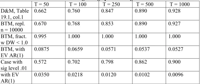
To provide support for McCallum’s 1993 argument, which is more suggestive than conclusive, consider the simulation results reported in Table 19.1 of Davidson and MacKinnon (1993). There the standard case of a spurious regression between two independently-generated random-walk variables is examined in that table’s column 2, which shows much greater rejection frequencies than the actual 0.05 for the true hypothesis of a zero slope coefficient—this is the spurious finding.2 For convenience, we report several of the Davidson and MacKinnon
frequencies in the first row of Table 1 below, where T designates sample size for the regressions studied via numerous replications. Of course we cannot use the same data as that generated by Davidson and MacKinnon, but we have generated results using the same simulation setup. Our rejection frequencies, analogous to those of Davidson and MacKinnon, are shown in row 2; they indicate clearly that our simulation study reproduces the incorrect rejections noted by Davidson and MacKinnon.3 Then in row 3, we report the fraction of times in which the regressions’ DW (Durbin-Watson, 1951) statistics are below 1.0, a value that implies extremely strong auto-correlation of the estimated residuals. As is clear from the table, almost all of the regressions in the Davidson and MacKinnon version of the basic Granger-Newbold example feature very
1 Actually, the argument developed in McCallum (1993) is more general in scope; it is to the effect that one can
analyze many relationships by using either levels or first differences of variables so long as care is taken to have residuals that are not autocorrelated. The spurious regression application amounts to a special case. Hamilton (1994, p. 562) briefly mentions a similar suggestion, which appears in an unpublished paper by Stephen R. Blough.
2 The innovations for the random-walk series are standard normal variates.
strong autocorrelation. So next we ask, “What would happen if the econometrician re-estimated his equation using some standard technique such as iterated Cochrane-Orcutt?” In Table 1, row 4 reports results based on calculations provided by the “AR(1)” procedure built into EViews.4 As can be seen, when the simulated equation is estimated using the E-Views specification of an AR(1) disturbance, rather than presuming white noise disturbances, the proportion of rejection frequencies falls to 0.0875 and 0.0659 for sample sizes of T = 50 and T = 100, and to values very close to the true 0.050 for larger sample sizes. This is our basic result.
The last two rows of Table 1 repeat the foregoing comparison but with the true
significance level set at 0.01, rather than 0.05. Thus the fifth row reports the rejection frequency when no notice is taken of the serially correlated residuals, in the same manner (but with a 2.576 critical value) as in row 2. Clearly, the same tendency to reject the (true) hypothesis of no
relationship occurs as in row 2. But again the fraction of cases with DW statistics less than 1.0 is 1.000 for all sample sizes above 50 (and is 0.9929 in that case). So again we alter the regressions by inclusion of the EViews AR(1) procedure, with results reported in the final row. And again the rejection frequencies are reasonably close to the true 0.01 value for sample sizes of 50 and 100, and are quite close for larger sample sizes. Thus the evidence provided by these two examples suggests that the “spurious regression” phenomenon is actually not a matter of major concern when there is no evidence of autocorrelated residuals. In that argument I am of course assuming that the estimated relationship is correctly specified in terms of the variables and lags included. If it is not, omitted variable problems may be serious—an important but distinct matter. 3. Case With Stationary Series
More recent papers by Granger (2001) and Granger, Hyung, and Jeon (2001) have
4 The EViews AR(1) estimation procedure differs somewhat from the iterative Cochrane-Orcutt procedure. In
particular, it assumes an AR(1) disturbance process for the estimated regression and then uses nonlinear estimation of parameters, including the AR parameter, as discussed by Davidson and MacKinnon (1993, pp. 331-341).
emphasized that spurious estimated relationships occur not only between (or among) random-walk or “integrated” variables, but also stationary but highly autocorrelated time series variates. Consequently, Davidson and MacKinnon (2004, p. 611) have included results analogous to those of theirs reported above but with the two basic series generated not by random walks, but by first-order autoregressive (AR) processes, using an AR parameter value of 0.8. In this case the Davidson and MacKinnon rejection values are reported only in graphical, not numerical, form so the reporting of them in row one of Table 2, below, can be only approximate. The values from my own 10,000 simulations given in row two are, however, in full accord. These rejection frequencies do not rise with sample size, as in the random-walk cases of Table 1, but are greater than 1/3 in all of our simulations—over six times as large as the true rejection probability. But, as before, almost all of the test regressions have DW statistic values smaller than 1.0.
Accordingly, we again consider the outcomes that occur when the investigator employs the EViews AR(1) procedure when regressing one of the AR series on the other. Clearly, row three shows that with this adjustment the rejection frequencies become close to the true values built into the simulation study. Furthermore, the same comments apply to the cases shown in rows 4 and 5, in which the true rejection probability is 0.01, rather than 0.05. Thus these results, like those in Table 1, support our suggestion that the “spurious regression” phenomenon is actually not a matter of concern when account is taken of autocorrelated disturbances
4. Integrated Moving-Average Series
In a somewhat neglected passage in their 1977 book, Forecasting Economic Time Series, Granger and Newbold (1977, pp. 207-214) have anticipated the argument of the preceding sections to the effect that conscientious researchers will make adjustments when encountering evidence of autocorrelated residuals. They have gone on to argue, however, that in the case of
time series variables generated by integrated moving-average processes (rather than random walk or AR(1) processes), re-estimation while including first-order autoregressive disturbances will not suffice to eliminate spurious relationships. Their Table 6.6 on their page 214 indicates that with MA parameters from 0.2 to 0.8 for the two series, rejection frequencies are in many cases in the range 0.15-0.30 rather than the true 0.05.5 This finding is for the sample size of T = 50 and 1000 replications. A representative rejection frequency for the case with both MA parameters equal to 0.6 is shown in the first row of Table 3. In the second row, results for various sample sizes and 10,000 replications are reported; these indicate that the spurious
relationship does not disappear when larger samples are utilized.6 This finding is consistent with the Granger-Newbold argument.
It is the case, however, that strong indications of serially-correlated residuals are present in the regressions reported in row 2. Even DW statistics, despite being inappropriate for the type of correlation in question, show considerable evidence suggestive of departures from white noise.7 More conclusively, rows 3 and 4 show the frequency with which added terms,
representing disturbances with AR(2) or MA(1) components, as well as the AR(1) component assumed in row 2, yield t-statistics greater than 1.96 in absolute value. Accordingly, the researcher might sensibly re-estimate the relationship with a MA(1) term added.8 In that case, the frequency of rejection for the hypothesis of no relation between the X and Y series is shown
5 Here MA parameters are positive under the specification y
t = yt-1 + vt− θvt-1; the notational conventions of Granger
and Newbold have them negative.
6 The rejection frequency reported for T = 50 differs quantitatively from that of Granger and Newbold because of a
somewhat different autoregressive correction and/or the smaller number of replications in their study. Qualitatively, the procedure used here yields similar results to those shown in the Granger-Newbold table.
7 The fraction of DW values differing from 2.0 by more than 0.5 grows from 0.1535 with T = 50 to 0.9997 with T =
1000.
8 If both the AR(2) and MA(1) terms are included, the latter is significant a much greater fraction of the time with
sample sizes of 100 and larger. Indeed, with sizes of 250 and greater, the MA(1) term is significant on almost every run (9999 out of 10,000 for T = 250, and all cases with T = 500 or 1000) while the AR(2) term’s rejection frequency is approximately equal to its true significance level. If nevertheless the AR(2) term is included instead of the MA(2), as in row 3, the rejection frequencies for the spurious xt variable, comparable to those in row 5 of Table 3,
are: 0.1126, 0.1051, 0.0920, 0.0817, 0.0704.
for different sample sizes in row 5. Clearly, we again find the outcome that spurious indications of a nonexistent relation are not frequent with samples of size 50 or 100 and are basically absent with the larger samples.
5. Conclusions
Let us conclude with a very brief restatement of the argument. Our main point is that “spurious regression” relationships between random-walk or strongly autoregressive variables are generally accompanied by clear signs of severe autocorrelation in the residuals of the estimated relationships; then re-estimation taking account of potential autocorrelation tends to eliminate the appearance of non-existent relationships. This is shown to be the case by
simulation studies for both random-walk and autoregressive cases of the relevant time-series variables. The argument is that any investigator with even minimal training in econometrics would/should not conclude a time-series regression study with (e.g.) a Durbin-Watson statistic of less than 1.0. Then re-estimation with a standard autocorrelation “correction” is shown to result in test statistics that are, with even moderate sample sizes, very close to true significant levels. If the relevant time-series variables come from integrated moving-average processes, the simple first-order autoregressive correction is not adequate. But evidence of correlated residuals is present in this case as well, and re-estimation assuming ARMA(1,1) disturbances goes a long way toward elimination of the problem. Accordingly, it appears that, for reasonably careful econometricians, the spurious regression problem is itself arguably spurious.9
9 It has not been shown that highly autocorrelated residuals are a feature of all cases in which non-existent
relationships may spuriously appear to be present. The types of cases that that have been considered here— independent series that are random walks, or first-order autoregressive with large positive AR parameters, or integrated first-order moving-average series—are, however, those that are predominant in the literature.
References
Cochrane, D., and G. H. Orcutt, “Application of Least Squares Regression to Relationships Containing Autocorrelated Error Terms,” Journal of the American Statistical Association, 44, 1949, 32-61.
Davidson, R., and J. G. MacKinnon, Estimation and Inference in Econometrics. Oxford University Press, 1993.
Davidson, R., and J. G. MacKinnon, Econometric Theory and Methods. Oxford University
Press, 2004.
Durbin, J., and G. S. Watson, “Testing for Serial Correlation in Least Squares Regression I,” Biometrica 37, 1950, 409-428.
Granger, C. W. J., “Spurious Regressions in Econometrics.” In A Companion to Theoretical Econometrics, ed. B. Baltagi. Blackwell Publishers, 2001.
Granger, C. W. J., and P. Newbold, “Spurious Regressions in Econometrics,” Journal of Econometrics 2, 1974, 111-120.
Granger, C.W.J., and P. Newbold, Forecasting Economic Time Series. Academic Publishers, 1977. Granger, C.W.J., N. Hyung, and Y. Jeon, “Spurious Regressions with Stationary Series,”
Applied Economics 33, 2001, 899-904.
Hamilton, J.D., Time Series Analysis. Princeton University Press, 1994.
Hill, R.C, W.E. Griffiths, and G. C. Lim, Principles of Econometrics, 3rd Ed. Wiley, 2008. McCallum, B. T., “Unit Roots in Macroeconomic Time Series: Some Critical Issues,”
Federal Reserve Bank of Richmond Quarterly Review 79(2), 1993, 13-43. Stock, J. H., and M. W. Watson, Introduction to Econometrics. Addison-Wesley, 2007. Wooldridge, J.M., Introductory Econometrics, 3rd Ed. Thomson South-Western, 2006.
Table 1: Simulation Results Regarding Spurious Regressions: Random-Walk Series T = 50 T = 100 T = 250 T = 500 T = 1000 D&M, Table 19.1, col.1 0.662 0.760 0.847 0.890 0.928 BTM, repl. n = 10000 0.670 0.768 0.853 0.890 0.927 BTM, fract. w DW < 1.0 0.995 1.000 1.000 1.000 1.000 BTM, with EV AR(1) 0.0875 0.0659 0.0571 0.0537 0.0527 Case with sig level .01 0.572 0.702 0.798 0.862 0.900 with EV AR(1) 0.0350 0.0218 0.0120 0.0102 0.0096 Table 2: Simulation Results Regarding Spurious Regressions: Stationary Series
T = 50 T = 100 T = 250 T = 500 T = 1000 D&M(2004) Fig. 14.1 0.33-0.34 0.34-0.35 0.35-0.36 0.36-0.37 0.36-0.37 BTM, repl. n = 10000 0.339 0.350 0.360 0.360 0.358 BTM, with EV AR(1) 0.0645 0.0564 0.0484 0.0503 0.0516 BTM, with sig level .01 0.202 0.221 0.226 0.231 0.228 with EV AR(1) 0.0185 0.0136 0.0116 0.0109 0.0108 Table 3: Simulation Results Regarding Spurious Regressions: Two IMA Series (θ = 0.6)
T = 50 T = 100 T = 250 T = 500 T = 1000 G&N, 1979 0.187 BTM, repl.1 n = 10000 0.1655 0.1746 0.1691 0.1522 0.1324 Freq2 t(ar2)>1.96 0.4378 0.8826 0.9999 1.0000 1.0000 Freq3 t(ma1)>1.96 0.8825 0.9933 1.0000 1.0000 1.0000 Freq4 t(x)>1.96 0.1351 0.0791 0.0572 0.0556 0.0510
1Fraction of times reject H: coeff of x = 0 in regression of y on c, x, ar(1)
2Fraction in which t-stat for added AR(2) parameter exceeds 1.96 in absolute value. 3Fraction t-stat for added MA(1) parameter exceeds 1.96 in reg. of y on c, x, ar(1), ma(1) 4Fraction of times reject H: coeff of x=0 in regression of y on c, x, ar(1), ma(1).