Tampereen teknillinen yliopisto. Julkaisu 1331 Tampere University of Technology. Publication 1331
Hanxue Yang
Markov Chain Monte Carlo Estimation of Stochastic
Volatility Models with Finite and Infinite Activity Lévy
Jumps
Evidence for Efficient Models and Algorithms
Thesis for the degree of Doctor of Philosophy degree to be presented with due
permission for public examination and criticism in Festia Building, Auditorium Pieni Sali 1, at Tampere University of Technology, on the 13th of November 2015, at 12 noon.
Tampereen teknillinen yliopisto - Tampere University of Technology Tampere 2015
ISBN 978-952-15-3597-0 (printed) ISBN 978-952-15-3617-5 (PDF) ISSN 1459-2045
Abstract
A financial model plays a key role in the valuation and risk management of financial derivatives, and it serves as an important tool for investors to measure the risk exposure of
their portfolios and make predictions and decisions. However, the popular affine stochastic
volatility models without jumps, such as the Heston model, have been questioned in the finance literature in terms of their appropriateness for modelling stock prices and pricing derivatives. Many alternative model specifications have been proposed in recent decades,
including the specification of non-affine variance dynamics and the inclusion of Lévy
jumps. However, the complexity introduced by further model specifications leads to poor probabilistic properties, and hence most popular estimation methods are not applicable. The Bayesian estimation method is among the few that work. In this thesis, I discuss the role of new model specifications and investigate the performance of Bayesian estimation methods.
First, I use an extensive empirical data set to study how the use of infinite-activity Lévy jumps in stock returns and variance improves model performance. The stock returns and
variance are driven by diffusions and different Lévy jumps, including the finite-activity
compound Poisson jump and infinite-activity Variance Gamma and Normal Inverse
Gaussian (NIG) jumps. Moreover, the non-affine linear variance process is compared to
the affine square-root stochastic process. With the conventional Markov Chain Monte
Carlo (MCMC) algorithms, including the Gibbs sampler and Metropolis-Hastings (MH) methods, and the Damien-Wakefield-Walker method to cope with complicated posteriors,
eighteen different model specifications are estimated using the joint information of the
S&P 500 index and the VIX index for 1996–2009. There is clear evidence that in terms of the goodness of fit and option pricing performance, a relatively parsimonious model with
infinite-activity NIG jumps in returns and non-affine variance dynamics is particularly
competitive.
In the second part of the thesis, I examine the performance of advanced MCMC algorithms.
The efficiency of the MH algorithm has been questioned because of its slow mixing speed,
especially in the presence of high dimensions and a strong dependence between model parameters and state variables. Generally, a class of algorithms seeks to improve the
MH by constructing more effective proposals, and another combines the MCMC with
the Sequential Monte Carlo algorithms. To investigate, I first conduct simulation studies to compare the estimation performance of seven advanced Bayesian estimation methods
against the MH. Specifically, I use the affine Heston model, the affine Bates model, and an
affine model with NIG return jumps, and examine whether the different jump structures
affect the estimation results. Second, I estimate the non-affine model with NIG return
jumps using the joint information of the S&P 500 index and the VIX for 2002–2005 with selected algorithms that perform well in the simulation studies. The results of the simulation and empirical studies are mixed about the performance of the algorithms. The
Fast Universal Self-tuned Sampler algorithms are particularly competitive in generating virtually independent samples and achieving the fastest mixing with a fixed number of MCMC runs, and their performance is stable regardless of the model specifications. However, they are computationally expensive. The computational costs of the Particle
Markov Chain Monte Carlo (PMCMC) methods are much cheaper and also efficient in
mixing, and they perform best when estimating the models without jumps/with NIG jumps in the simulation studies, as well as in the fit to the VIX in the empirical studies. However, the PMCMC methods are more vulnerable to model specifications than the other algorithms; in particular, the rare large compound Poisson jumps in the Bates model significantly reduce the acceptance rate and worsen the estimation performance of the PMCMC methods.
Preface
The research presented in this thesis was carried out at the Department of Industrial Management at Tampere University of Technology between 2013 and 2015, within the Marie Curie Initial Training Network HPCFinance. During the writing of this thesis, I was financially supported by the European Union Seventh Framework Programme under grant agreement No. 289032.
I would like to express my sincere gratitude to my supervisor, Professor Juho Kanniainen, for giving me such an invaluable opportunity to work on the HPCFinance project, and more importantly, for his insightful guidance and consistent support that helped me
manage many difficult problems. In my research, I have always been encouraged by
his enthusiasm and honest criticism and advice. I am also especially grateful for the inspiring cooperation with, and support from, Professor Luca Martino, who proposed and developed the powerful FUSS algorithms and guided me in applying the algorithms to financial problems. In addition, I would like to express my gratitude to the pre-examiners, Professor Michael Johannes and Professor Andreas Kaeck, for their helpful comments and suggestions.
Furthermore, I wish to thank my colleagues at the Department of Industrial Management and in the HPCFinance project. In particular, I thank Milla Siikanen, Sindhuja Ran-ganathan, Jaakko Valli, and Binghuan Lin in the finance group for the helpful discussions
and activities outside of work. Special thanks go to my officemates, Jun Hu and Ye Yue,
for providing a fun and stimulating work environment. I am also thankful to the project managers, Dr. Santiago Velasquez and Dr. Hanna-Riikka Sundberg, and the department secretary, Ms. Heli Kiviranta, for their assistance and administrative support.
I want to thank Jukka Annala and his wife Tuija for inviting me to their beautiful home and summer cottage. I will never forget the journey into the deep forest and the experiences of taking a sauna and jumping into the cold lake, picking mushrooms, and tasting karjalanpiirakka. A special mention goes to the lovely couple Huiling Wang and Tinghuai Wang. I am glad to have friends like you, who have made my life here unforgettable.
Last but not least, I owe my deepest thanks to my parents and my dearest grandmother for their endless encouragement and love. Thank you for sharing your lives with me. You remain my best friends, no matter how far away you are.
Contents
Abstract i
Preface iii
Acronyms vii
1 Introduction 1
1.1 Background and Motivation . . . 1
1.2 Questions and Research Methods . . . 6
1.3 Outline and Contributions of the Thesis . . . 8
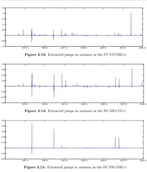
2 Jumps and Volatility Dynamics for the S&P 500 Index: Conventional MCMC 13 2.1 Description of Models and Notations . . . 13
2.2 Change of Measure . . . 16
2.3 VIX . . . 19
2.4 Estimation Method . . . 21
2.5 Data Description and Option Pricing Settings . . . 25
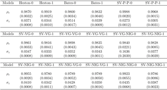
2.6 Estimation Results . . . 28
2.7 Discussion . . . 45
3 Model Estimation with Advanced MCMC Algorithms: Simulation Studies 47 3.1 Motivation . . . 47
3.2 Review: Conventional MCMC Methods . . . 48
3.3 Particle Filters . . . 50
3.4 Advanced MCMC Methods . . . 51
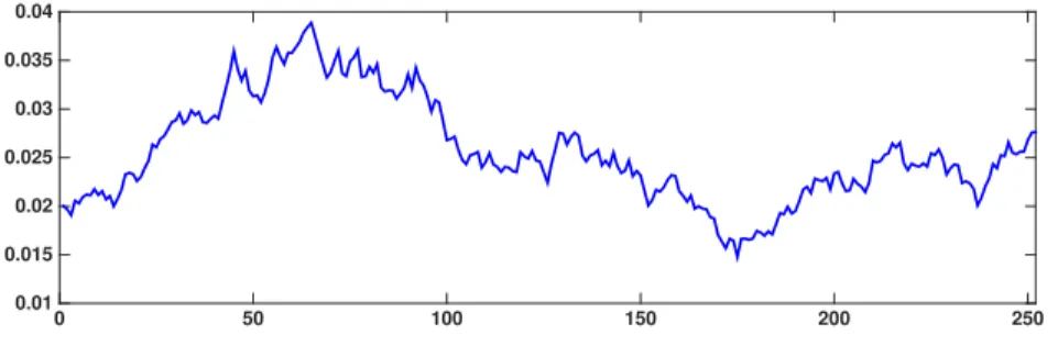
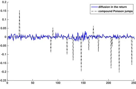
3.5 Simulation Studies: Data Generation . . . 56
3.6 Implementation of Algorithms . . . 58
3.7 Results . . . 62
3.8 Discussion . . . 76
4 Model Estimation with Advanced MCMC Algorithms: Empirical Studies 79 4.1 Motivation . . . 79 4.2 Data . . . 80 4.3 Implementation of Algorithms . . . 81 4.4 Results . . . 82 4.5 Discussion . . . 96 v
5 Discussion and Conclusion 97
Bibliography 101
Appendices 109
A Simulation Studies: Extracted Variance 111
B Simulation Studies: Extracted Jumps 117
C Empirical Studies: Extracted Variance of the SV-NIG-1 Model 121
Acronyms
ACF Autocorrelation Function
AM Adaptive Metropolis
APF Auxiliary Particle Filter
AR Acceptance Rate
ARMS Adaptive Rejection Metropolis-Sampling
ARS Adaptive Rejection Sampling
BS Black-Scholes
CBOE Chicago Board Options Exchange
CEV Constant Elasticity of Variance
DIC Deviance Information Criterion
DWW Damien-Wakefield-Walker
FUSS Fast Universal Self-tuned Sampler
LL Log-Likelihood
MC Monte Carlo
MCMC Markov Chain Monte Carlo
MH Metropolis-Hastings
MLE Maximum Likelihood Estimation
MSE Mean Squared Error
NIG Normal Inverse Gaussian
PDF Probability Density Function
PF Particle filter
PG Particle Gibbs
PGAS Particle Gibbs with Ancestor Sampling
PMCMC Particle Markov Chain Monte Carlo
PMMH Particle Marginal Metropolis Hastings
RC Rejection Chain
RMSE Root Mean Squared Error
RS Rejection Sampling
SMC Sequential Monte Carlo
SQR Square Root
VG Variance Gamma
1 Introduction
1.1 Background and Motivation
A financial model can be regarded as an approximation of the true dynamics of a financial asset. It is a mathematical model that uses variables to abstract parameters of interest and is designed to capture some of the most important empirical features of the financial market. It enables us to introduce randomness and make assumptions on the basis of
market observations to link the variables representing different features of the market and
different types of risk, and more importantly, to quantify and evaluate the risk and make a
useful analysis. The financial model is a key element of the valuation and risk management of complicated financial derivatives and an important tool for investors to estimate future returns, measure the risk exposure of their portfolios, and make predictions and decisions.
1.1.1 Financial Models
The empirical evidence has shown that the Black-Scholes (BS) model proposed by Black and Scholes (1973) fails to provide a satisfactory description of the dynamics of real-life stock prices. That is, the stock prices are not log-normally distributed; rather, the distribution of stock returns is usually negatively skewed and has long and fat tails and high peaks. More importantly, jumps, especially downside jumps, may occur randomly in the path of the stock price. If investors base their investment and risk management decisions on a model that misses the fundamental features of stock prices, they will be exposed to a substantial risk of loss.
In response, many more flexible and realistic models have been proposed for stock prices, such as the stochastic volatility model and the model with Lévy jumps.
Stochastic volatility models
As its name suggests, the stochastic volatility model replaces the constant volatility in the BS model with another random variable described by some stochastic process. The Heston model (Heston, 1993) is one of the most popular stochastic volatility models. It describes the spot variance as a mean-reverting square-root (SQR) process that is driven by a Brownian motion correlated with the Brownian innovation in the process of the stock returns. By assuming a negative correlation between two Brownian innovations in
returns and variance, the Heston model takes account of the volatility feedback effect,
that is, changes in stock returns and variance are negatively correlated. Moreover, the introduction of stochastic volatility can alter the skewness and kurtosis of the distribution of stock prices. Yet the performance of the Heston model has been questioned in the literature. Jones (2003) argues that the stochastic volatility model with an SQR variance process is unable to generate realistic variance dynamics, and he concludes that the
Constant Elasticity of Variance (CEV) model is more consistent with index returns and option prices and is, hence, a better choice for describing the variance process. Similar
observations have been made in many finance studies. For instance, Christoffersen et al.
(2010a) suggest that the stochastic volatility model with linear diffusion for variance,
compared to SQR diffusion, is much better in the aspects of modelling the realised
volatility and index returns and pricing options.
Moreover, in the historical time series of stock returns and realised variance, many fre-quent small jumps and some large jumps typically occur randomly, and while stochastic volatility models may resolve some empirical biases of the BS model, they do not account for unexpected frequent jumps. The Bates model proposed by Bates (1996) augments the Heston model by adding a compound Poisson jump component to the dynamics of stock returns. However, the results in both Bates (2000) based on options and Pan (2002) based on the joint information of stock prices and options suggest that the Bates model fails to trace systematic variations in option prices, and that a model with jump components in
the variance process is highly useful. Duffie et al. (2000) propose the double-Poisson-jump
model as a generalisation of the Heston, Bates, and Merton jump diffusion models. This
model is constructed by adding another compound Poisson jump component to the vari-ance process, whose jump times and sizes are simultaneous and correlated, respectively, with those in stock returns. Eraker et al. (2003) examine the double-Poisson-jump model using return data, and their empirical results are clearly in favour of this model rather than the Heston and Bates models, because the double-Poisson-jump model success-fully captures unexpected large jumps. Consequently, Eraker et al. (2003) argue that the inclusion of a double-Poisson-jump specification might be indispensable, especially under extreme market conditions. However, when models are estimated and compared using the joint information of index returns and option prices, the inclusion of jumps in variance seems less important, as Eraker (2004) and Kaeck and Alexander (2012) point out.
Lévy processes
Most of the finance literature relies on the use of Brownian motion to capture normal asset price variations and on compound Poisson jumps to capture large price movements in returns and variance. In fact, both Brownian motion and compound Poisson jump belong to the class of Lévy processes. By definition, a Lévy process is a stochastic process, the distribution of whose increments is stationary and independent of its past track. According to the behaviour of the Lévy measure, a Lévy process can be classified in terms of jump activity: finite activity and infinite activity. A finite-activity Lévy process can generate only a finite number of small and large jumps in a finite time interval. Brownian motion and the compound Poisson process are two examples of the finite-activity Lévy process. In contrast, the infinite-activity Lévy process can generate an infinite number of small jumps; however, the number of large jumps can only be finite because the Lévy process is often assumed with càdlàg paths. Importantly, infinite-activity jumps are more flexible to generate distributions with desired kurtosis, skewness, or tails.
Over the years, a number of option pricing models with infinite-activity Lévy jumps have been proposed, such as the Variance Gamma (VG) model (Madan et al., 1998), the
Normal Inverse Gaussian (NIG) model (Barndorff-Nielsen, 1997b,a), the CGMY model
(Carr et al., 2002), and the finite moment log stable process (Carr and Wu, 2003). Carr et al. (2003) propose the time-changed Lévy model and incorporate stochastic volatility into the Lévy process through an instantaneous time change, and the resultant model
1.1. Background and Motivation 3 Moreover, Wu (2005) conducts an extensive analysis of the empirical performance of
different types of time-changed Lévy models discussed in Carr et al. (2003).
Combination of stochastic volatility and jumps
Combining stochastic volatility models and infinite-activity Lévy jumps may further improve model performance, but this specification has not been widely studied. Two notable exceptions are Li et al. (2008) and Yu et al. (2011). Specifically, they compare
affine SQR stochastic volatility models with infinite-activity VG and Log Stable (LS)
jumps in the return process, without jumps in the variance process, against the Bates model and the double-Poisson-jump model. The models are estimated using the S&P 500 index returns in Li et al. (2008) and the joint information of the S&P 500 index returns and short-term ATM SPX option prices in Yu et al. (2011). Their empirical results show that models with infinite-activity Lévy jumps significantly outperform the Bates and double-Poisson-jump models in goodness of fit and achieve better performance
in the option pricing test in Yu et al. (2011). More recently, with a discrete-time affine
GARCH model, Ornthanalai (2014) estimates five types of infinite-activity Lévy jumps using the joint information of index returns and option prices by the maximum likelihood estimation (MLE) method, and suggests that infinite-activity jumps, rather than Brownian
motion, should be “the default modelling choice” for option valuation. The difference
between my research and theirs lies mainly in the use of non-affine variance dynamics
and infinite-activity variance jumps.
Previous empirical studies have not focused on whether the use of jumps in both the
return and variance processes can obviate the non-affine variance process, or vice versa.
One interesting paper is Kaeck and Alexander (2012), which uses an extensive data set
to estimate and compare the model specifications of the non-affine linear variance process
and the CEV process with the inclusion of a finite-activity compound Poisson jump structure in the return and variance processes. Kaeck and Alexander (2012) conclude that
the inclusion of compound Poisson jumps is less important than allowing for non-affine
dynamics. The main difference between my research and Kaeck and Alexander (2012)
lies in the use of infinite-activity Lévy jumps.
Surprisingly, very little research focuses on the empirical option pricing performance of stochastic volatility models with infinite-activity Lévy jumps in both variance and returns,
especially with non-affine variance dynamics, perhaps due to computational challenges.
The first part of this thesis aims to fill this gap.
Overall, empirical research with long-term data sets, including booms and crises, is
necessary for making robust conclusions on the empirical performance of different types
of infinite-activity jumps and non-affine variance dynamics. The recent literature contains
only a few papers that use the joint information of returns and options to study model performance with infinite-activity Lévy jumps. Some exceptions include Yu et al. (2011), Li (2011), and Ornthanalai (2014). In this thesis, I use the S&P 500 index returns and option prices via the 30-day VIX index from January 1996 to December 2009, a 14-year period in which several financial crises occurred, to estimate the models. The VIX is computed by averaging the weighted prices of SPX call and put options with the target maturity over a wide range of strike prices, and under certain model assumptions, it measures the square root of expected integrated variance over the horizon defined by the target maturity. Since the VIX index is computed from a portfolio of option prices, it contains aggregated information about option prices and can be used to derive the risk-neutral dynamics of a model. It is worth mentioning that the optimal strategy is
using option prices directly to estimate models, because the VIX index averages out the
information contained in option prices. However, because I consider both the affine and
non-affine models in this thesis, I employ the VIX index, instead of option prices, to
estimate the risk-neutral model parameters. Specifically, since the characteristic functions
of non-affine models are not available in closed form, the efficient Fast Fourier Transform
(FFT) proposed in Carr and Madan (1999) is not applicable. Therefore, with option prices, time-consuming Monte Carlo methods should be used to estimate the models.
However, since the closed-form formula of the VIX index can be derived in all the affine
and non-affine models discussed in this thesis, using the VIX enables me to estimate the
non-affine models efficiently. Several previous studies, such as Ait-Sahalia and Kimmel
(2007), Duan and Yeh (2010), Kaeck and Alexander (2012), and Kanniainen et al. (2014),
have already confirmed the effectiveness of using the VIX for estimating the risk-neutral
model dynamics.
1.1.2 Bayesian Estimation Methods
Many financial research papers apply the classic MLE method to estimate and compare models (see, for example Ait-Sahalia and Kimmel, 2007; Bates, 2006). However, the application of the MLE requires that the form of the joint probability density function (PDF) of the data and the specifications of the moments of the joint PDF should be known. It also requires that the joint PDF be evaluated for all parameter values. Therefore, although the MLE has proved excellent for model estimation, its application is limited. Many other estimation methods with relaxed assumptions are employed in finance studies, such as the Generalised Method of Moments in Andersen and Sørensen (1996) and Chacko
and Viceira (2003), the Efficient Method of Moments in Chernov and Ghysels (2000),
and the Method of Moments techniques used in Pan (2002). However, these estimation techniques require that the moments be fully specified, although the assumption of a fully-specified distribution in the MLE is removed.
In contrast, Bayesian estimation methods do not have the above requirements. Their implementations by means of sophisticated Monte Carlo techniques (Liu, 2004; Robert and Casella, 2004) have become very popular over the last two decades. In particular, Bayesian methods have recently gained popularity in the finance research and have been applied
to estimate complicated financial models (see, for example, Christoffersen et al., 2010a;
Eraker et al., 2003; Kaeck and Alexander, 2013a; Li, 2011, and reference therein). First, Bayesian methods are very flexible and can combine the information of index returns and options prices. Second, Bayesian methods allow for not only estimating the parameters but also extracting the latent state variables of models, such as jumps and variance. Third, as general and flexible tools for simulating complicated stochastic processes, Bayesian methods can be combined with other estimation methods. For example, when integrated with the MLE, they can solve the problem of a likelihood that is not known in closed form (see, for example, Jacquier et al., 2007; Johansen et al., 2008).
One shortcoming of Bayesian methods is that they are typically implemented on the basis of approximation. In most cases where Bayesian methods are employed, we cannot
directly sample from the true distribution that we are interested in, that is,p( , X|Y),
where is the parameter set,X represents the latent state variable, and Y represents
the data. Bayesian methods try to approximate the true distribution by generating approximate samples, and this has plagued designers of Bayesian estimation algorithms since the beginning. Although the literature contains powerful mathematical theory for assessing the mixing and accuracy of Bayesian methods, such as the asymptotic and limit
1.1. Background and Motivation 5
theories, in many problems, it is difficult to assess the approximating performance of
Bayesian algorithms.
Generally, there are two classes of Bayesian estimation methods: Sequential Monte Carlo (SMC) and Markov Chain Monte Carlo (MCMC). MCMC algorithms generate samples from a target distribution by drawing from a simpler proposal distribution (Liang et al., 2010; Liu, 2004) and by generating a Markov chain. SMC algorithms, or particle filters, use a finite set of particles to represent the target distribution and compute probabilistic properties on the basis of the particle set. SMC algorithms are on-line estimation methods, which means that when a new observation arrives, the particles can be updated to account
for the information brought by the new observation; in contrast, off-line MCMC algorithms
have to be restarted. However, since particle filters were originally designed for extracting latent state variables in a model, they were not capable of dealing with estimation involving unknown, fixed model parameters. In the past two decades, although there have been various adaptations of particle filters aimed at simultaneously handling the estimation of state variables and unknown fixed parameters, their performance must be tested further. Conversely, MCMC algorithms are typically flexible in dealing with problems of estimating parameters and state variables, but the mixing speed of the Markov chain, which is the key to the success of MCMC algorithms, can be very slow, especially when the proposal is poorly selected.
In the past decade, numerous new Bayesian estimation methods have been proposed, targeted at solving the problems of conventional MCMC algorithms in the presence of high dimensions, complicated target distributions, and complex patterns of dependence between stable variables and parameters. The second part of this thesis seeks to apply these
methods to estimate different financial models and compare their estimation performance.
The Adaptive Metropolis (AM) algorithm, introduced by Haario et al. (1999a, 2001), aims
to develop an effectiveGaussianproposal by updating its variance on the basis of past
samples generated in the MCMC chain. According to Haario et al. (1999a, 2001, 2006), the MCMC chain generated by this on-line tuning proposal is no longer Markovian or reversible. However, according to Haario et al. (2001), under some regularity conditions about how the adaptation is conducted, the chain is ergodic and retains the desired stationary distribution.
Moreover, several automatic and self-tuned samplers have been proposed for dealing with more general proposals, such as Adaptive Rejection Sampling (ARS) (Gilks, 1992; Gilks and Wild, 1992), Adaptive Rejection Metropolis Sampling (ARMS) (Gilks et al., 1995, 1997; Meyer et al., 2008), Independent Doubly Adaptive Rejection Metropolis Sampling (Martino et al., 2012, 2014), and Adaptive Sticky Metropolis (Martino et al., 2013). Generally, these algorithms construct the proposals with a number of support points, and adaptively modify the proposals by adding new points. However, the ARS cannot dealing with log-concave target distributions, since it is based on the rejection sampling technique and the proposal must always be above the target. In the ARMS, support points cannot be added inside regions where the proposal is below the target. Moreover, the performance of the above algorithms is dependent on the choice of initial
support points, and it is difficult to ensure their ergodicity, especially in applications
within the Gibbs sampler (Gilks et al., 1997; Robert and Casella, 2004). Recently, the Fast Universal Self-tuned Sampler (FUSS) algorithm (Martino et al., 2015) is proposed
to overcome the above drawbacks. The FUSS algorithms construct effective self-tuned
proposals, starting with a large number of support points, and then remove many of them according to some pruning scheme combining relevant information. The numerical
experiments in Martino et al. (2015) show that FUSS algorithms are able to generate virtually independent samples in the presence of high dimensions and spiky distributions. Alternatively, it is possible to make use of an SMC algorithm as the proposal distribution within an MCMC algorithm. More specifically, an SMC algorithm can be used to approximate the likelihood to be used within a standard Metropolis-Hastings (MH) algorithm, and the resultant algorithm can be regarded as an approximation to a marginal
MH that targets the marginal posteriorp( |Y) of the joint posteriorp( , X|Y), where
Y represents the data, represents the set of parameters in a model, andX represents
the latent state variables. This approach, called Particle Marginal Metropolis-Hastings (PMMH) in Andrieu et al. (2010), is used in some literature (see, for example, An and Schorfheide, 2007; Fernández-Villaverde and Rubio-Ramírez, 2005), and Andrieu et al. (2010) prove the convergence of the algorithm, such that to ensure the convergence of the
generated chain, the resampling algorithm should be unbiased, so that the estimation error produced by the approximation does not change the equilibrium distribution. Andrieu et al. (2010) also propose a new scheme called Particle Gibbs (PG) sampler, which can be regarded as an approximation of the Gibbs sampler that targets the joint posterior
p( , X|Y). In Andrieu et al. (2010), the PMMH and PG sampler are collectively called
Particle Markov Chain Monte Carlo (PMCMC) methods. The PG sampler uses a so-called conditional SMC update to ensure that the PG kernel leaves the exact target distribution invariant. In a conditional SMC update, a pre-specified reference trajectory of latent state variables with an ancestral lineage survives after all the resampling steps. After a complete run of the SMC update, a new reference trajectory is selected from the particle set with probabilities given by the importance weights of the particles. However, as underlined in Lindsten and Schön (2013) and Chopin and Singh (2013), a potential problem with the PG sampler is that in the presence of high dimensions, the path degeneracy is inevitable and the mixing of the chain may be poor. This problem is addressed by the Particle Gibbs with Ancestor Sampling (PGAS), proposed in Lindsten et al. (2014), by adding a backward sampling step to the PG sampler. Numerical experiments show that this backward sampling step can significantly improve the mixing speed of the chain, even with a small number of particles.
While some finance research applies the conventional MCMC or SMC algorithms to estimate stochastic volatility models with jumps, few attempts have been made to apply the above newly proposed algorithms. Indeed, the problem of estimating stochastic
volatility models with jumps is particularly difficult because of the strong dependence
between parameters and state variables and the model complexity brought by jump components. Therefore, it would be interesting to examine how the advanced estimation methods perform in estimating complicated financial models compared to the conventional MCMC algorithms.
1.2 Questions and Research Methods
This research is divided into two parts. The first part of the research focuses on
esti-mating and comparing different model specifications, namely, the inclusion of return
jumps of finite or infinite activity to the stochastic volatility model, affine/non-affine
variance dynamics, and the inclusion of variance jumps correlated with return jumps. Eighteen model specifications are estimated from an extensive data set using conventional MCMC algorithms and are then compared in terms of goodness of fit and option pricing performance. The second part focuses on the application and comparison of advanced
1.2. Questions and Research Methods 7 Bayesian estimation methods, with the aim to identifying a method that is capable of
efficiently estimating the unknown fixed model parameters and latent state variables
in the presence of high dimensions, strong dependence between parameters and state variables, and complicated target distributions.
In the first part of my research, I study the models with infinite-activity return jumps,
augmented with correlated infinite-activity variance jumps and specifications of affine and
non-affine variance dynamics. I use both VG and NIG jumps, which are popular examples
of infinite-activity pure jump processes; the VG of finite variation with a relatively low arrival rate of small jumps; and the NIG of infinite variation with a sample path that may have infinite total variation in any bounded time interval, almost surely. These models are compared against the benchmark Heston model without any jump component and the Bates and double-Poisson-jump models with finite-activity compound Poisson jumps. This research aims to answer the following questions:
– Do inclusions of infinite-activity jump components in returns and variance and the
use of a non-affine variance process improve the goodness of fit and option pricing
performance, as compared to the standard SQR models with or without finite-activity compound Poisson jumps (the Heston, Bates, and double-Poisson-jump models)?
– In particular, which Lévy jump, VG or NIG, in returns and variance, better describes the return and variance dynamics and prices options?
– Moreover, how do Lévy jumps of finite activity and infinite activity differ in capturing
jumps in returns and variance?
These are important questions because there is a trade-offbetween model accuracy and
a real computational challenge due to the need for Monte Carlo methods in the option
pricing that use double-infinite-activity-jump models or non-affine models.
In the first part of the research, I estimate the models using the joint information of the S&P 500 index returns and option prices via the 30-day VIX index from January 1996 to December 2009, a 14-year period with several financial crises. The models are estimated with conventional MCMC algorithms, including the Gibbs sampler, the MH
algorithm, and the Damien-Wakefield-Walker (DWW) method to increase efficiency.
After the estimation, I compare the model performance in terms of goodness of fit and option pricing errors in two sample periods: January 1996–December 2009 and January 2010–December 2010. The option prices are computed with the Monte Carlo method, and instead of using the realised return time series or a simulation method to predict the daily spot variance when pricing multiple daily cross-sections of options, I use the VIX-based technique to extract the time series of daily spot variance, as in Kanniainen et al. (2014). The results in Kanniainen et al. (2014) clearly show that this technique can
improve the option pricing performance across different models, including the NGARCH
and the Heston-Nandi models, over the traditional approach of estimating spot variance from realised returns.
In the second part of the research, I examine the performance of advanced MCMC algorithms. The algorithms comprise the AM, the FUSS, the PMMH, and the PGAS. I aim to answer the following questions:
– Do inclusions of jump components of finite or infinite activity affect the estimation performance?
– Can the problems of conventional MCMC algorithms be solved, or at least alleviated, by using advanced MCMC algorithms?
– Which algorithm performs best with a fixed length of chain?
– What are the advantages and disadvantages of each algorithm in estimating the financial models?
I first conduct simulation studies to compare the performance of algorithms. In the
simulation studies, I simulate one-year data of index returns and variance from the affine
Heston and Bates models and the affine model with NIG return jumps and then use
the simulated index returns as observations to estimate the model parameters under the
physical measure. Then I examine the performance of algorithms with different chain
lengths and numbers of particles in the PMMH and PGAS algorithms and compare the algorithms in terms of the parameter estimates, extraction of variance and jumps, acceptance rate, and the likelihood of the estimation result. Next, I apply the advanced MCMC algorithms to more complex problems with a large volume of empirical data.
Both the physical and risk-neutral dynamics of the non-affine model with NIG return
jumps, which performs best in the model comparison part, are estimated using the joint information of the S&P 500 index returns and option prices via the 30-day VIX index from January 2002 to December 2005. Besides the aspects compared in the simulation studies, I employ the estimated model to price the index options in 2002–2010, and compare the option pricing performance.
1.3 Outline and Contributions of the Thesis
This thesis is divided into five chapters. The contents of each chapter are summarised as follows. Chapter 1 briefly introduces the financial models and Bayesian estimation methods and describes the motivation, objectives, and contributions of the thesis. Chapter 2 describes the physical and risk-neutral dynamics of the models studied in this thesis, explains the application of the conventional MCMC estimation methods, and presents the empirical results. Chapter 3 introduces the general ideas and designs of advanced MCMC algorithms, explains their applications to selected financial models, and presents the estimation results using the simulated data. Chapter 4 focuses on the application of advanced MCMC algorithms to model estimation using the empirical data. Chapter 5 concludes the thesis.
The empirical results in the first part are summarised as follows. First and most
im-portantly, the inclusion of infinite-activity return jumps is critical for non-affine (linear)
variance specification. In particular, the non-affine model with infinite-activity NIG
return jumps significantly outperforms the affine and non-affine models with and without
finite-activity return jumps in both goodness of fit and option pricing. Its performance is
also clearly better than that of the non-affine model with VG return jumps. Interestingly,
the performance of infinite-activity VG and NIG return jumps is mixed with the affine
(SQR) variance specification, suggesting that using unrealistic affine variance dynamics
may negatively affect the identification of the models’ jump components. Overall, it is the
combination of infinite-activity NIG jumps in the return process and non-affine variance
1.3. Outline and Contributions of the Thesis 9 Second, the role of activity variance jumps is less important than that of infinite-activity return jumps. Obviously, in terms of goodness of fit, the relatively parsimonious
non-affine model with NIG return jumps is almost as good as the more complex models
with infinite-activity jumps in both the return and variance processes. In terms of option
pricing, the non-affine model with NIG return jumps performs best among all the models
that I test, including the complex models with return and variance jumps. Moreover, variance jumps are insignificant for the models with NIG jumps in returns, since they worsen the goodness of fit and cause a small improvement only in the option pricing test
with affine models. However, according to the goodness-of-fit results, if one still prefers
using a model with infinite-activity jumps in both returns and variance, the inclusion of NIG variance jumps, rather than VG variance jumps, in the models with VG return jumps is more appropriate. This is plausible because the NIG is of infinite variation and is more capable of capturing the frequent small jumps in the variance dynamics than the finite-variation VG.
The above findings provide two financial economic insights. First, although the Bates and double-Poisson-jump models may capture rare, large jumps with the finite-activity compound Poisson jumps, they miss a large number of frequent small jumps that may cause potential substantial losses in investment and risk management. On the other hand, the inclusion of infinite-activity jumps in the return process better captures the uncertainty of future jumps, generates more realistic return dynamics and option prices, and obviates the complex models with variance jumps. In particular, the infinite-variation NIG process as return jumps produces a larger jump risk premium than the finite-variation VG process and outperforms the VG in goodness of fit and option pricing.
Second, despite the popularity of tractable affine models in derivative pricing, my research
results clearly demonstrate the dominance of non-affine models over affine ones in goodness
of fit and option pricing, which is in line with the recent literature (see, for example,
Christoffersen et al., 2010b; Kaeck and Alexander, 2012). More importantly, the non-affine
variance specification improves model robustness, whereas the affine variance specification
may lead to unstable option pricing performance between different samples. It may be
dangerous to use affine models for making investment and risk management decisions;
therefore, decision makers must seriously consider the trade-off between computation
time and model robustness.
In the second part of my research, I note that different jump structures significantly affect
the estimation performance of algorithms. The results of the simulation studies show that the algorithms fail to distinguish the randomness created by the infinite-activity jumps
and Brownian diffusions in the return process of the affine model with NIG return jumps.
This makes parameter estimation and variance extraction very challenging, and the extra complexity introduced by the NIG jumps requires the FUSS and PMCMC methods to increase the numbers of MCMC runs and particles, while the MH and AM are less capable of dealing with the complicated model specification. Compound Poisson jumps create
rare but significant changes in the return process of the affine Bates model, which are
distinctive of the diffusions; therefore, all the algorithms perfectly extract the compound
Poisson jumps when estimating the affine Bates model. However, the inclusion of rare,
large return jumps significantly reduces the acceptance rates of the PMCMC methods, and thus their estimation performance deteriorates. In contrast, the other algorithms are less vulnerable to the specification of compound Poisson jumps and performs consistently
in estimating different models.
that for models with a simple specification, the MH is very competitive owing to its low computational cost. However, if the target distribution is complicated or the proposal of the MH is inappropriate, the acceptance rate may be very low, and most generated draws are wasted. The AM makes use of the previous samples and dynamically tunes the proposal, and this online-tuned adaptive proposal can significantly raise the acceptance rate and speed up the convergence of the chain. Moreover, in the presence of a spiky and complicated target distribution and high-dimensional state variables, numerous MCMC iterations may be required for the chain generated by the MH and AM to converge.
The FUSS algorithms can tackle this problem by constructing an efficient proposal
and producing virtually independent samples, as noted in Martino et al. (2015). A shortcoming of the FUSS algorithms is that with a fixed number of MCMC iterations, they are slower than the very fast MH and AM algorithms. However, if one focuses on achieving a good estimation performance, despite the relatively high computational cost, the FUSS algorithms are very competitive due to their fast and good mixing properties. In addition, the PMCMC methods can deal with complicated target distributions and strong dependence between parameters and state variables, and their computational cost is significantly lower than that of the FUSS algorithms, making them very competitive. However, when the other algorithms achieve a stable estimation performance across
different model specifications, the performance of the PMCMC methods depends largely
on the properties of the specific problem, and their performance may deteriorate when the dependence between state variables is weak. Moreover, as pointed out in Lindsten et al. (2014), the relative performances of the PMMH and PGAS depend on whether the ideal marginal MH or the Gibbs sampler, that is, the samplers that PMMH and PGAS approximate, respectively, has the better mixing property for the specific problem. In estimating the Heston-0 and SV-NIG-0 models, the PGAS outperforms the PMMH and the other algorithms with a small number of MCMC iterations and particles, suggesting the fast and good mixing of the PGAS kernel in estimating these two models.
In the empirical studies, the adaptive proposal used in the AM increases the acceptance rate of the MH and reduces the autocorrelation between samples of the spot variance. The FUSS-RC and PGAS further improves the extraction of the spot variance in that the autocorrelation functions (ACFs) of the spot variance extracted by the FUSS-RC and PGAS drop sharply. Furthermore, the FUSS-RC even reduces the ACF with negative
autocorrelation, suggesting that the chain is efficient in generating good representatives of
the target distribution. In contrast, the acceptance rates of the PMMH algorithms are very low owing to the model specification of independent NIG return jumps, and jump-related parameters are poorly identified by the PGAS. This suggests that compared to the MH, AM, and FUSS-RC, the PMCMC methods are less capable of extracting independent
jumps; moreover, the inclusion of independent jumps may negatively affect the estimation
performance of the PMCMC methods. Furthermore, the choice of estimation methods
affects the option pricing performance. In particular, the model-implied VIX based on
models estimated with the PMMH-PF1 almost completely coincides with the market VIX; therefore, since the option pricing performance is highly correlated with the fit to the VIX, the PMMH-PF1 outperforms the other algorithms in the option pricing test. In contract, the PGAS performs the worst in all three option samples owing to the poorly identified jump-related parameters under the risk-neutral measure. The MH is the second best algorithm in predicting option prices due to the use of realised variance as the initial variance, which leads to an estimation result consistent with the market conditions in 2006–2010.
1.3. Outline and Contributions of the Thesis 11 dependence between parameters and state variables, and if one emphasises the fit to observations that can be represented as a function of model parameters and state variables, the PMMH-PF1 is very competitive. However, the performance of the PMMH-PF1 and the PGAS may be weakened by the inclusion of independent jumps. In contrast, the other algorithms are less vulnerable to the inclusion of independent jumps, and they achieve a stable performance in parameter estimation, extraction of state variables, fit to the VIX, and option pricing. In particular, an appropriate choice of initial values for state variables can significantly improve the performance of the MH; moreover, the FUSS-RC is very competitive because it can improve the estimation performance of the MH and AM and generate good representatives of the target distribution of state variables in the presence of high dimensions and a strong dependence structure.
Finally, I declare that I am the sole author of this thesis. Although this PhD thesis is a monograph and is not presented as a collection of papers, it relates to three papers that I
have co-authored. First, Chapter 2 is closely related to Yang and Kanniainen (2015).1
For this paper, I coded the MCMC algorithms, estimated the models, and mainly wrote the paper. Prof. Kanniainen mainly coded the option pricing framework and participated in the writing.
The estimation results in Chapters 3 and 4 have not been reported in any previous paper, but part of the results are obtained by the FUSS algorithms proposed by Martino
et al. (2015).2 This paper presents the key idea and design of the FUSS algorithms and
uses numerical experiments to illustrate their estimation performance compared to other MCMC methods. For this paper, I coded the external MCMC algorithm to estimate a stochastic volatility model with VG return jumps, estimated the model using simulated data, and wrote the financial example. I did not code the FUSS algorithms that were applied inside the external MCMC.
Kanniainen et al. (2014)3present an efficient way to employ information of the VIX index
in option valuation, which I also employ in this thesis. For this paper, I participated in implementing the MLE method and I had a minor role in the writing.
1Yang, H. and J. Kanniainen (2015), “Jump and Volatility Dynamics for the S&P 500: Evidence for
Infinite-Activity Jumps with Non-Affine Volatility Dynamics from Stock and Option Markets”, submitted toReview of Finance(under revision).
2Martino, L., H. Yang, D. Luengo, J. Kanniainen, J. Corander (2015),“A Fast Universal Self-tuned
Sampler within Gibbs Sampling”, forthcoming inDigital Signal Processing.
3 Kanniainen, J., B. Lin, and H. Yang (2014), “Estimating and Using GARCH Models with VIX
2 Jumps and Volatility Dynamics for
the S&P 500 Index:
Conventional MCMC
In this chapter, I compare 18 stochastic volatility models with finite/infinite-activity Lévy
jumps in returns, or in both returns and variance, and with affine/non-affine variance
dynamics in terms of goodness of fit and option pricing errors. The models are estimated with conventional MCMC algorithms using the joint information of the S&P 500 index returns and 30-day VIX index reformulated from option data during 1996–2009. This chapter seeks to answer the following questions:
• Do the inclusion of infinite-activity jump components in returns and variance and
the use of a non-affine variance process improve the goodness of fit and the option
pricing performance, compared to the standard SQR models with or without finite-activity compound Poisson jumps (the Heston, Bates, and double-Poisson-jump models)?
• In particular, which Lévy jump, VG or NIG, in returns and variance, better describes the return and variance dynamics and prices options?
• Moreover, how do Lévy jumps of finite/infinite activity differ in capturing jumps in
returns and variance?
The outline of this chapter is as follows. Section 2 introduces the affine and non-affine
models with finite/infinite-activity jumps and describes the change of measure. In Section 3, I derive the formulae of the model-implied VIX index and assume a relation between the market VIX and model-implied VIX. Section 4 describes the estimation method. Section 5 describes the data set and option pricing methods. Section 6 presents the empirical results, including parameter estimation, extracted jumps, goodness of fit, and option pricing errors. Section 7 concludes the chapter.
2.1 Description of Models and Notations
In this part, I briefly describe the models to be compared in this chapter. First, the types of Lévy jumps considered here comprise the compound Poisson jump, which is of finite activity, and the VG and NIG jumps, which are of infinite activity. Second, stochastic
volatility is generated by diffusion and Lévy jumps that are correlated with jumps in
the return process. Moreover, apart from the conventional SQR variance process, the
non-affine variance process with the linear diffusion term is used.
Lévy processes are used because of their flexible distributions, whereas Brownian motion, as a special type of Lévy process with continuous paths, restricts itself to following the symmetric normal distribution. The Lévy process may generate any path as long as the distribution of the increments of the path is stationary and independent of its past track, and the path does not have to be continuous. When used in a model to fit a real-life stock price, the Lévy process may help resolve some known empirical biases of the BS model, such as the realised skewness and excess kurtosis in the distribution of stock returns, and may capture the jump risks that are missed by the BS and Heston models.
As in Carr and Wu (2004) and Tankov (2003), the Lévy process can be classified in terms
of jump activity according to the behaviour of the Lévy measurefi: iffisatisfies
⁄ Œ ≠Œ
fi(dx)<Œ,
the Lévy process is of finite activity. This implies that s|x|<1fi(dx) < Œ and that
s
|x|Ø1fi(dx)<Œ; therefore, the Lévy process can have only a finite number of both small
and large jumps per unit of time. However, iffi satisfies
⁄ Œ ≠Œ
fi(dx) =Œ,
the Lévy process is of infinite activity. This means that this Lévy process can generate an infinite number of small jumps and a finite number of large jumps per unit of time, becauses|x|<1fi(dx) =Œands|x|Ø1fi(dx)<Œ, where the latter inequality is entailed by
the definition of the Lévy process. As pointed out in Li et al. (2008), the infinite-activity Lévy process can generate small jumps for the path of stock returns that are too big for Brownian motion, and too small and frequent for the finite-activity compound Poisson process, to capture.
Let{Yt}be the continuously compounded return of the S&P 500 index, and let {vt}be
the instantaneous squared volatility of the return. Then under the physical measureP,
I assume that the return dynamics of the S&P 500 index is described by the following
stochastic differential equations:
dYt = 3 µt≠12vt+„PJ(≠i) 4 dt+ÔvtdWY,t+dJY,t, (2.1) dvt = ŸP(◊P≠vt)dt+–v—t(fldWY,t+ 1≠fl2dWv,t) +dJv,t, (2.2)
where WY,t andWv,t are mutually independent Brownian motions. JY,t andJv,t are
Lévy jumps in the return and variance processes, respectively, of finite or infinite activity.
„P
J(u) is calculated fromEP[eiuJY,t] =e≠t„
P
J(u), and it measures the expectation ofeJY,t
because EP[eJY,t] = e≠t„PJ(≠i); therefore, EP[St], the expectation of the index price St=eYt, equalsS0EP[e
st
0µsds], as in Madan et al. (1998). µtis the physical time-varying
drift of the index return,ŸP is the physical rate of the mean reversion ofv
t,◊P represents
the physical long-term mean ofvt,–controls the diffusion term in the variance process,
andflcontrols the correlation betweenYtandvtand captures the leverage effect. The
parameter— determines whether the variance dynamics is an affine SQR process or a
non-affine linear process. The linear specification is often called the continuous-time
2.1. Description of Models and Notations 15
2.1.1 Benchmark Models: Heston, Bates, and Double-Poisson-Jump
Models
The models considered as benchmarks are the Heston, Bates, and double-Poisson-jump models. The last model has contemporaneous jumps in both returns and variance
occurring at random times, depending on the increments of the Poisson processNtwith
intensity ⁄: JY,t= Nt ÿ i=1 ›iY, Jv,t= Nt ÿ i=1 ›vi, Nt≥Poisson(⁄t). (2.3)
The size of jumps in the variance process follows an exponential distribution: ›v
t ≥exp(µv),
whereµv is the scale parameter. The reason for choosing the exponential distribution for
variance jumps is to ensure the positiveness of these jumps given the economic observation that realised variance typically demonstrates large, positive jumps. The size of jumps in the return process follows a normal distribution with the mean correlated with the jumps
in variance: ›Y
t |›vt ≥N(µy+flJ›tv,‡y2), whereflJ models the correlation between return and variance jumps. The double-Poisson-jump model nests the Bates model by removing
the variance jumps,Jv,t, and the Heston model by removing bothJY,tandJv,t.
In this thesis, the double-Poisson-Jump models are labelled SV-P-P-0 when— = 0.5 and
SV-P-P-1 when— = 1 (the notation comes fromStochasticVolatility, compoundPoisson
jumps in returns, and compound Poisson jumps in variance). Similarly, the Heston and
Bates models are labelled SV and SV-P, respectively, but for simplicity, their existing names are used and the models are labelled Heston-0, Heston-1, Bates-0, and Bates-1,
depending on the values of—.
2.1.2 Infinite-Activity Lévy Jumps
First, the VG and NIG jumps are added only in the return process, and the resultant
models are labelled SV-VG-ior SV-NIG-i, according to the choice of return jumps and
values of—. The VG process can be defined by subordinating a Brownian motion with
drift “and variance‡by an independent Gamma processGY with a unit mean rate and
a variance rate‹:
JY,t(‡,“,‹) =“GY,t(‹) +‡WY,GY,t(‹) (2.4)
and its Lévy measure is
fiV G(dx) = e≠M xdx ‹x , x >0; fiV G(dx) = e≠N|x|dx ‹|x| , x <0, (2.5) where M = A 1 2“‹+ Ú 1 4“2‹2+ 1 2‡2‹ B≠1 , (2.6) N = A ≠12“‹+ Ú 1 4“2‹2+ 1 2‡2‹ B≠1 . (2.7)
Similarly, an NIG process can be obtained by subordinating a Brownian motion with
time that a Brownian motion with drift‹ reaches the positive levelt. The Lévy measure of the NIG is fiN IG(dx) = ‡– fi e—xK 1(–|x|) |x| dx, (2.8)
where–=‹2/‡2+“2/‡4,—=“/‡2, andK1 is the modified Bessel function of the third
kind with index 1. The NIG is also of infinite activity; moreover, it is of infinite variation. A Lévy process is of infinite variation if the total variation of its sample path in any bounded time interval is infinite, almost surely, for any partition of the time interval. When the VG is of finite variation and hence can only have jump-type discontinuities and is bounded in any bounded interval, the infinite-variation NIG is more flexible and, therefore, a potential candidate for good performance in modelling financial time series. Further, an infinite-activity Lévy jump component, VG or NIG, is added to the variance process, motivated by the findings in Eraker et al. (2003), which indicate the necessity of jumps in the variance process to account for extreme market conditions. The models
obtained with infinite-activity jumps in returns and variance are labelled SV-VG-VG-i,
SV-VG-NIG-i, SV-NIG-VG-i, and SV-NIG-NIG-i, i= 0,1, according to the choices of
return and variance jumps and the values of—.
The structure of the jumpsJv in variance is similar to that ofJY in returns, regardless of
the jump subordinator:
Jv,t(‡v,“v,‹v) =“vGv,t(‹v) +‡vWv,Gv,t(‹v). (2.9)
Here,Gv(‹v) can be an inverse Gaussian or Gamma process, independent of the other
random sources. Wv,Gv is the base Brownian motion correlated withWY,GY byflv, as in
Eberlein and Madan (2009).
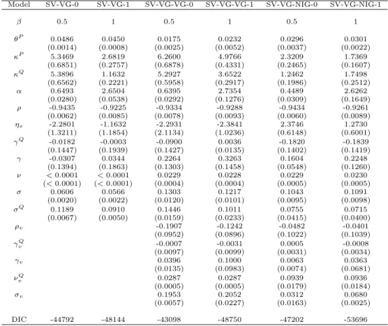
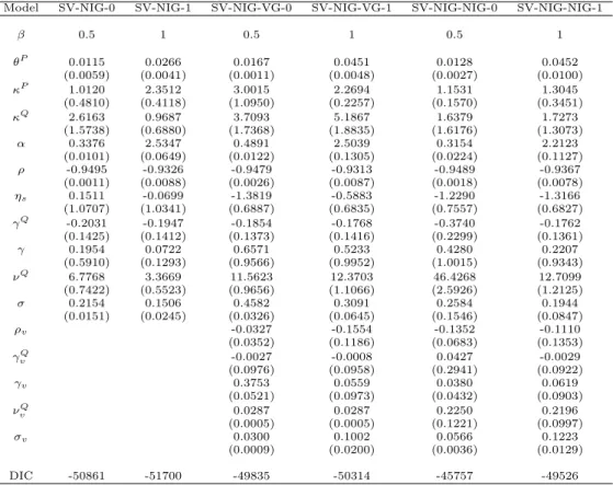
Overall, there are18 different model specifications, and they are summarised in Table 2.1.
2.2 Change of Measure
In this section, I describe the risk-neutral dynamics and the change of measure.
I follow the procedure described in Pan (2002) to define the change of the probability measure for Brownian motions in the return and variance processes in all the models
characterised above. Briefly, assuming two risk premia,÷sand÷v, the change of measure
for Brownian motions is as follows:
dWY,t(Q) = dWY,t≠÷sÔvtdt (2.10) dWv,t(Q) = dWv,t+ 1 1≠fl2 A fl÷s+ ÷v –v—t≠0.5 B Ôv tdt. (2.11)
In defining the change of measure for the Lévy jumps in returns, I follow the practice in Yu et al. (2011). Under the Sato theorem, which states the relation between the physical and
risk-neutral measures of the Lévy process, and the restriction that the jumpJY(Q) under
Qis still a VG jump, a change of measure forJY exists if‹P =‹Q, while“Qand‡Qmay
change freely. For a compound Poisson jump, all jump-related parameters can change
freely betweenP andQ; however, for simplicity and econometric meaning, onlyµQ
y is assumed to change freely. For models with an NIG jump component in returns, the Esscher
2.2. Change of Measure 17
Table 2.1: Model acronyms and specifications
Model name Heston-0 Heston-1
0.5 1
Jump in return None
Jump in variance None
Model name Bates-0 Bates-1
0.5 1
Jump in return compound Poisson
Jump in variance None
Model name SV-P-P-0 SV-P-P-1
— 0.5 1
Jump in return compound Poisson Jump in variance compound Poisson
Model name SV-VG-0 SV-VG-1
— 0.5 1
Jump in return Variance Gamma
Jump in variance None
Model name SV-VG-VG-0 SV-VG-VG-1
— 0.5 1
Jump in return Variance Gamma
Jump in variance Variance Gamma
Model name SV-VG-NIG-0 SV-VG-NIG-1
— 0.5 1
Jump in return Variance Gamma
Jump in variance Normal inverse Gaussian
Model name SV-NIG-0 SV-NIG-1
— 0.5 1
Jump in return Normal inverse Gaussian
Jump in variance None
Model name SV-NIG-VG-0 SV-NIG-VG-1
— 0.5 1
Jump in return Normal inverse Gaussian Jump in variance Variance Gamma
Model name SV-NIG-NIG-0 SV-NIG-NIG-1
— 0.5 1
Jump in return Normal inverse Gaussian Jump in variance Normal inverse Gaussian
remains of the NIG type, with the same‡P and‡Q and the same–P N IG= (‹ P)2 (‡P)2 + (“P)2 (‡P)4 and–QN IG= (‡(‹QQ))22 +(“ Q)2 (‡Q)4, but a different—N IGQ = “P (‡P)2 and—N IGQ = “Q (‡Q)2. It can be
easily worked out that the restriction on the values of risk-neutral jump-related parameters ‡Q,“Q, and‹Q is‡P =‡Q,!‹P"2= (‹Q)2(‡Q)2+(“Q)2≠(“P)2
(‡Q)2 , and“Q can change freely.
In fact, under a pure NIG jump model for stock price dSt =St≠dJt, whereJt is an
NIG jump process,—N IGQ and“Q can be worked out from the other jump parameters
and a constant risk-free interest rate. However, in reality, the risk-free interest rate may
vary, and as the model structure becomes complicated, it is difficult to compute—N IGQ .
Consequently, in the estimation,“Q is identified from the VIX data.
Given the change of measure for the jumps and diffusion terms, the Radon-Nikodym
derivative for the models is dQ dP|t= exp ; ≠ ⁄ t 0 ’Y,sdWY,s≠ ⁄ t 0 ’v,sdWv,s≠ 1 2 5⁄ t 0 ! ’Y,s2 +’v,s2 " ds 6< eUt, (2.12)
where eUt is defined in the Sato theorem (details can be found in Sato, 1999) and ’
Y
and’v are the market prices of risks of Brownian innovations in returns and variance,
respectively, defined as ’Y,t = ≠÷sÔvt, (2.13) ’v,t = 1 1≠fl2 A fl÷s+ ÷v –vt—≠0.5 B Ôv t. (2.14)
Therefore, under the risk-neutral measureQ, the return and variance follow
dYt = 3 rt≠ 1 2vt+„QJ(≠i) 4 dt+ÔvtdWY,t(Q) +dJY,t(Q), (2.15) dvt = ŸQ(◊Q≠vt)dt+–vt— 1 fldWY,t(Q) + 1≠fl2dWv,t(Q) 2 +dJv,t(Q),(2.16)
Here,„QJ(≠i) is the jump compensator forJY under measureQ, and its form depends on
the specific type ofJY:
„Q,CP oissonJ (u) = ⁄ A 1≠eiuµ Q y≠12‡2yu2 1≠iuµvflJ B , (2.17) „Q,V GJ (u) = log !1 ≠iu“Q‹+1 2u2‹(‡Q)2" ‹ , (2.18) „Q,N IGJ (u) = ≠‹Q+‡ Ú u2≠2iu“ Q ‡2 + (‹Q)2 ‡2 . (2.19) The form of„P
J in Equation (2.1) is the same as„
Q
J, except that the risk-neutral parameters
should be changed to the corresponding physical ones. Furthermore,
÷svt = rt≠µt+„QJ(≠i)≠„PJ(≠i), (2.20)
÷v = ŸQ≠ŸP, (2.21)
where rt is the risk-free interest rate and ŸQ is the mean-reverting speed under the
2.3. VIX 19
In the variance dynamics under Q,
ŸQ(◊Q≠vt) =ŸP(◊P≠vt)≠÷vvt. (2.22)
This implies that◊QŸQ =◊PŸP. In the estimation, the physical◊P is estimated from
the data, and◊Q is computed by◊Q=ŸP◊P/ŸQ.
2.3 VIX
In this section, I briefly introduce the construction of the VIX index from the option data
(market VIX) and derive its pricing formula in different model settings (model-implied
VIX). Finally, I quote an assumption that suggests a relation between the market and model-implied VIX.
The VIX measures the square root of expected integrated variance over the horizon defined by the target maturity, and it is computed by averaging the weighted prices of SPX puts and calls with the target maturity over a wide range of strike prices. Importantly, there are two reasons why I have chosen the VIX index, not option prices directly, to estimate the risk-neutral model parameters. First, the VIX index, computed from a portfolio of
option prices, contains aggregated information about option prices1 and can be used to
derive the risk-neutral dynamics of a model. Second, the efficient FFT is not applicable
to non-affine models because their characteristic functions are not available in closed
form. Therefore, with option prices, one should use the Monte Carlo method to estimate the models, an extremely time-consuming process, or approximation methods (see, for
example, Lewis, 2000). However, since the formula of the VIX index under all the affine
and non-affine models discussed in this chapter can be derived in closed form, using the
VIX can make the model estimation efficient. Several previous studies, such as Ait-Sahalia
and Kimmel (2007), Duan and Yeh (2010), Kaeck and Alexander (2012), and Kanniainen
et al. (2014), have confirmed the effectiveness of using the VIX, instead of option prices,
for estimating the risk-neutral model dynamics.
Specifically, according to the definition published in 2003 by the Chicago Board Options Exchange (CBOE), the theoretical value of the squared VIX is
VIX2 t,T ◊10≠4= 2 Te rT t(Ft(t+T), t+T), (2.23)
whereFt(t+T) is the forward price of the stock with maturityt+T at timet, and where
t(K0, t+T) = ⁄ K0 0 Pt(K, t+T)dK K2 + ⁄ Œ K0 Ct(K, t+T)dK K2 . (2.24)
Here,Ct(K, t+T) andPt(K, t+T) are the European call and put option prices at time
t, with maturityt+T and strike price K. As in Duan and Yeh (2010), by the generic
payoffexpansion result of Carr and Madan (2001), the theoretical value of the squared
VIX can be reduced to
VIX2 t,T ◊10≠4= 2 T 3 ≠logF St t(t+T)≠ EQ 5 logSt+T St 64 . (2.25)
1It is worth mentioning that the optimal strategy for estimating the risk-neutral dynamics is using
option prices directly to estimate models, because the VIX index averages out the information contained in option prices.
According to the model assumption in my setting, VIX2 t,T ◊10≠4 = 2 T ⁄ t+T t rsds≠ 2 T 3 ⁄ t+T t rsds+T(MJ+„QJ(≠i)) (2.26) ≠12EQ C⁄ t+T t vsds D 4 , (2.27) = ≠2(MJ+„QJ(≠i)) + 1 TE QC⁄ t+T t vsds D . (2.28)
Here, the jump compensators„QJ(≠i) for compound Poisson, VG, and NIG jumps are
specified in Section 2.2. MJ is the expected mean size of the return jumps underQ. For
the VG jump,MJ =“Q, for the NIG jump,MJ =“Q/‹Q, and for the compound Poisson
jump,MJ=⁄(µQy +flJµv).
The average integrated variance under the risk-neutral measureQis
EtQ A⁄ t+T t vsds B =vt 1≠e≠ŸQT ŸQ + ◊PŸP+M v ŸQ A T≠1≠e≠ ŸQT ŸQ B , (2.29)
whereMv is the expected mean size of the variance jumps underQ. IfJv is a VG jump,
Mv=“vQ. IfJv is an NIG jump,Mv =“vQ/‹vQ. In the models SV-P-P-i,Mv=⁄µv.
Moreover, the target maturityT is annualised. When a 30-day VIX is computed and if
the calendar day count convention is used, obviouslyT = 30/365. However, I use the
trading day count convention, because the return data are recorded on a trading day basis
(see also Kanniainen et al., 2014). Thus, in my setting,T = 22/252, as there are 252
trading days per year and 22 trading days per month. In addition, since the CBOE uses calendar days to calculate the VIX (see CBOE’s documentation), squared observations on the VIX must be multiplied by (30/365)(252/22) when the trading day count convention is applied.
From the VIX index, we can estimate model parameters under the risk-neutral measure
Qand use the estimated model for option pricing. Since all the models in this chapter