SPATIALLY REGULARIZED LOW RANK TENSOR OPTIMIZATION FOR VISUAL DATA
COMPLETION
Jianchao Gao
?Hong Shi
?Wenwu Wang
†?
School of Computer Science and Technology, Tianjin University, Tianjin, China
†Department of Electrical and Electronic Engineering, University of Surrey, Guildford, UK
ABSTRACT
Low-rank tensor completion is a recent method for estimating the values of the missing elements in tensor data by minimiz-ing the tensor rank. However, with only the low rank prior, the local piecewise smooth structure that is important for vi-sual data is not used effectively. To address this problem, we define a new spatial regularization S-norm for tensor comple-tion in order to exploit the local spatial smoothness structure of visual data. More specifically, we introduce the S-norm to the tensor completion model based on a non-convex LogDet function. The S-norm helps to drive the neighborhood ele-ments towards similar values. We utilize the Alternating Di-rection Method of Multiplier (ADMM) to optimize the pro-posed model. Experimental results in visual data demonstrate that our method outperforms the state-of-the-art tensor com-pletion models.
Index Terms—tensor completion, S-norm, LogDet func-tion, low rank, visual data processing
1. INTRODUCTION
In practical applications, the data captured often contain miss-ing values due to the failure of storage device, packet loss in transmission, and incomplete measurement in data collection. The goal of completion is to recover the unknown elements based on the known elements. The basic methods for deal-ing with this problem are local [1], which utilize the adjacent relationship but do not capture the global information. Re-cently, a global model has been proposed for addressing the completion problem, e.g. using the tensor rank minimization model [2, 3, 4, 5, 6].
For tensor completion, Liu et al. proposed to use the Sum of Nuclear Norm (SNN) to approximate the tensor rank [7]. Since the tensor rank is more sensitive to small singu-lar values, Huang et al. proposed a truncated nuclear norm minimization (TNNM) method for tensor completion [8], in which a higher recovery accuracy is obtained by eliminating smaller singular values. The calculation of the tensor nuclear norm is expensive, therefore a parallel matrix factorization
The work is partly supported by National Natural Science Foundation of China under Grant 61502335.
method is proposed in [9]. The tensor train (TT) rank is used to replace Tucker rank in [10], leading to the Tmac-TT al-gorithm that works better than Tmac. Simultaneous tensor decomposition and completion (STDC) is presented in [11] by utilizing a graph-Laplacian based Tucker decomposition. However, the matrix nuclear norm does not behave well in some cases, e.g. when the elements of matrix are sampled uniformly. In order to overcome these limitations, a non-convex rank approximation has been considered by Zhao et al. [12] where the log-determinant (LogDet) function is used to approximate the rank function. The effectiveness of LogDet has been widely verified in several applications, such as sub-space clustering [13], recommender system [12], and tensor completion [14].
Due to the presence of the object edges, visual data are often only piecewise smooth. For visual data completion, it is not sufficient to only consider the low rank prior. To ad-dress this, total variation (TV) is used for completion prob-lem. For example, TV has been combined with matrix fac-torization [15], or SNN and Tucker decomposition, leading to LRTC-TV-I, and LRTC-TV-II [16]. Although the tensor completion model based on the TV-norm has achieved great performance, it does not make full use of the neighborhood information of each missing element. Chen et al. proposed a new spectral spatial (SS) regularization method to exploit local smoothness, and applied it successfully to change de-tection in hyperspectral imagery [17]. Inspired by this work, we generalize SS regularization for the matrix to higher-order tensors and define the S-norm as the spatial regularization for tensor. More specifically, we add the S-norm based spa-tial regularization to the tensor completion model based on a non-convex LogDet function. To optimize this model, we present an Augmented Lagrangian Multiplier (ALM) method with Alternating Direction Minimizing (ADM) strategy [18]. To summarize, the key contributions of this work are as fol-lows:
•We propose a new spatial regularization S-norm to ex-ploit the property of the local piecewise smoothness of visual data.
• We combine the S-norm with the non-convex LogDet function to build a tensor completion model.
datasets show that our model outperforms the state-of-the-art tensor completion methods.
1.1. Notation
In this paper, a scalar is denoted by lowercase lettersx, and a matrix is denoted by capital letters,X ∈ Rm×n which is
composed of column vectors, denoted as(xxx1, xxx2,· · ·, xxxn),
wherexxxi ∈ Rm, i = 1,· · ·, n. AnNth-order tensor is de-noted by calligraphic lettersX ∈RI1×I2×···×IN, and the
el-ements ofX are denoted asxi1,i2,···,iN, where1≤ik ≤Ik,
1≤k≤N. The mode-n unfolding ofX is a matrixX(n)of sizeIn×I1· · ·In−1In+1· · ·IN, i.e,X(n) =U nf oldn(X).
On the contrary, its reverse operator is denoted asF old(·), andX =F oldn(Xn). The operation for a tensor is similar to
those for a matrix. kX kF denotes the Frobenius norm of the tensorX.
2. THE PROPOSED METHOD 2.1. Tensor Spatial Regularization
For a matrix dataA∈ RM×N, Chen et al. [17] propose the SS regularization that exploits local spatial patterns and its definition is given as follows:
kAkSS= I P i=1 J P j=1 W2−1 P k=1 wkij a0ij−akij 2 2, (1)
whereakij is thekth neighbor of the center elementa0ij,k·k2 denotes the`2-norm of the matrix, andwkij is the weight of
thekth neighbor ofa0
ij.W2−1is the number of neighbors.
For visual data completion, to preserve the local smooth-ness structure, we generalize the SS regularization from the matrix to higher-order tensors. We propose the following def-inition for S-norm as a tensor spatial regularization:
kX kS= N X n=1 λn X(n) SS, (2)
whereX is a tensor of sizeI1×I2× · · · ×IN, andλn’s are
tuning parameters. For the third-mode visual data, its mode-1 and mode-2 matricizations help preserve the spatial structure, so we setλ1, λ2= 1, andλ3= 0.
2.2. LogDet and S-norm for Tensor Completion
We consider tensor completion by integrating a non-convex LogDet function with the spatial regularization. Given an Nth-order incomplete tensor X ∈ RI1×I2×···×IN, our
method starts with both the global information and the lo-cal structure of the tensor data. Specifilo-cally, the incomplete tensor is reconstructed by the global low rank prior of the data. The S-norm helps to smooth the reconstructed data, by driving the nearby elements to have similar values. The
objective function is written as:
min X τkX kS+ N X n=1 αnlogdet X(n) T X(n) 1/2 +ηnIn s.t. PΩ(X) =PΩ(T), (3)
whereτis a regularization parameter. T is the given incom-plete tensor with missing elements andXhas the same size as T.PΩ(·)is an operator, which chooses entries that is equal to 1 inΩ.Inis then-th identity matrix. Given the constant array α
αα= [α1, α2,· · · , αN],αn satisfiesαn ≥0,Pnαn = 1. Ω
is an index set where the index of observation elements can be either “1” or “0”.ηnis a constant, satisfyingηn>0.
2.3. Optimization Algorithm
Our objective function (3) consists of a non-convex rank ap-proximation constraint and a spatial prior. Since the unfolded matrices share the same entries, they cannot be solved in-dependently. To address this issue, we introduce additional variables{Mn}Nn=1 and{Hn}Nn=1 to separate these interde-pendent terms. As a result, Eq. (6) can be converted to the following equivalent problem:
min X,Mn, Hn τ N X n=1 λnkHnkSS+ N X n=1 αnlogdet MnTMn 1/2 +ηnIn s.t. PΩ(X) =PΩ(T), Mn=X(n), Hn=X(n), (4)
Each variable can be updated alternatively with other vari-ables fixed. Firstly, we define an effective strategy based on the ALM method with the ADM strategy [18]. Eq. (4) can be solved by the following ALM problem:
L(X, Mn, Hn, Yn,Λn) = N X n=1 λn∗τkHnkSS + N X n=1 αn∗logdet MnTMn 1/2 +ηnIn + N X n=1 αn∗ X(n)−Mn, Yn +µ1 2 X(n)−Mn 2 F + N X n=1 λn∗ X(n)−Hn,Λn +µ2 2 X(n)−Hn 2 F , (5) whereYn,Λn are Lagrange multipliers, µ1, µ2 are positive penalty scalars and h·,·i denotes the matrix inner product. Then, we can apply the alternative projection strategy to up-dateX, Mn, Hn, Yn,Λn, i.e., updating one of the variables
with the others fixed, so we separate a large-scale problem into the following four smaller subproblems.
1. Update1. Update1. Update Mk+1
n : Given Xk, Hnk, Ynk,Λkn, we solve the
following optimization problem:
Mnk+1= arg min Mn N X n=1 αn∗ logdet MnTMn 1/2 +ηnIn + N X n=1 αn∗ µk 1 2 X(kn)−Mn+ Yk n µk 1 2 F ! . (6)
In order to solve Eq. (6) effectively, we use the Theorem 1 in [19] to deal with the tensor case. Based on this theorem, defineA = Xk (n)− 1 µk 1 Yk
n. We can obtain the closed form
solution of Eq. (6), written as:
Mnk+1=U diag(proxf,uk
1(σA)−diag(v
k
))VT, (7) whereU,V,σAare obtained by the singular value
decompo-sition (SVD) ofA.proxf,uk
1(·)is the Moreau-Yosida operator
[19].vk= [1 σk1 Mnk+ηn
,· · · ,1 σ1k Mnk+ηn
]. 2. Update2. Update2. UpdateHk+1
n : GivenXk, Mnk+1, Ynk,Λkn, we solve the
following optimization problem:
Hnk+1= arg min Hn N X n=1 λn∗ τkHnkSS+ µk 2 2 kHn−Jk 2 F . (8) LetJ =Xk (n)− 1 µk 2
Λkn. Taking the derivative with respect to Hnand setting it to zero, we get
h h hkr+1= 1 P iccc k i Dkrccc k Hnk+1= [hhh k+1 1 , hhh k+1 2 ,· · ·, hhh k+1 In ] T , (9) where i = 1,2,· · ·, W2, Dk r ∈ RI1···In−1In+1···IN×W 2 , and the matrix Dk
r = [hhh k(1)
r ,· · ·, hhh
k(W2−1)
r , jjjr]. jjjr is
column vector of J. The coefficient vector is denoted as
ccck = [w
1, w2,· · ·, wW2−1, 1
2τµ k
2]. So the variableHnk+1can
be easily obtained by solving Eq. (9). 3. Update3. Update3. UpdateXk+1: GivenHk+1
n , Mnk+1, Ynk,Λkn, the closed
form solution to the least squares problem is obtained as:
Xk+1= P n[F oldn(µk1M(n)+Ynk)+F oldn(µk2H(n)+Λkn)] PN n=1(αnµk1+λnµk2) Ω . TΩ (10) 4. Update4. Update4. Update multipliers: GivenXk, Mk+1
n , H k+1
n , we have
the following update equations:
Ynk+1=Y k n +µ k 1 X(kn+1) −M k+1 n Λkn+1= Λkn+µk2 X(kn+1) −H k+1 n . (11)
The pseudocode is summarized in Algorithm 1.
3. EXPERIMENTS
In this section, we illustrate the experimental results for vi-sual data, namely the color image completion and medical data completion. We compare our method with the existing algorithms, such as FaLRTC and HaLRTC [7], TmacTT [10], STDC [11], LRTC-TV-I and LRTC-TV-II [16] and LogDet
Algorithm 1:Optimization Procedure of LRTC-S
Input:input anNth-order corrupted tensorT, and index setΩ.
Output:recovered tensorX
1 Initialize these variables
Hn0=Mn0= 0, Yn0= Λ0n= 0, PΩ X0
=PΩ(T),
µmax= 1010, max iter= 500, ηn=ε= 10−6, ρ= 1.05, µ0
1=µ02= 10−4, α, λ;
2 whilenot convergeddo
3 Update variablesMnk+1according to Eq. (7); 4 Update variablesHnk+1according to Eq. (9); 5 Update variablesXk+1according to Eq. (10); 6 UpdateYnk+1,Λkn+1according to Eq. (11); 7 Check the convergence conditions; 8 Updateµk1+1=ρµk1;µk2+1=ρµk2. 9 end
[14]. Our model is implemented by the Tensor Toolbox for MATLAB1. For convenience, we use three metrics to evaluate the performance of our algorithm, namely the relative squared error (RSE), peak signal-to-noise ratio (PSNR)[16], and structural similarity (SSIM) [20]. In our experiments, we use the relative error of two adjacent iterations as the criterion to show convergence, i.e,Xk− Xk−1
F Xk F ≤ε. The
other parameters of our algorithm are initialized as follows. We tuneτfrom set{0.001,0.005,0.01,0.1}, which gives the best performance. We setW = 3, andw1,3,6,8, w2,4,7,9are chosen from values in{1,2,3,4}.
3.1. Color image completion
First, we choose seven classic color images, namely airplane, lena, baboon, barbara, house, peppers and sailboat. Each im-age is represented as a third order tensor with size256×256×
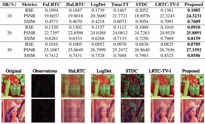
3. In the experiment, we randomly remove many pixels of each image, and the missing rate is ranged from 65% to 95%. In Table 1, we have listed the comparison of seven algorithms on the color image that are recovered at 10%, 20%, and 30% sampling rate (SR), i.e. missing rate at 90%, 80%, and 70% respectively. Each value in the table is the average based on the seven images. It can be seen that LogDet and TmacTT algorithms behave similarly and they are better than FaLRTC and HLRTC at 20% and 30% sampling rate, but their perfor-mances are worse than STDC and LRTC-TV-I. However, our proposed model is superior to the other baselines. In particu-lar, when the sampling rate is 10%, the RSE of the proposed model is only 0.1085. In order to intuitively show the ery performance of our method, Figure 1 presents the recov-ery results of five algorithms on two color images with 95% missing rate. We can see that LogDet has better performance
Table 1. Comparison of different algorithms on color image
SR(%) Metrics FaLRTC HaLRTC LogDet TmacTT STDC LRTC-TV-I Proposed
10 RSE 0.1894 0.1847 0.1739 0.1467 0.2052 0.1361 0.1085 PSNR 19.6037 19.8018 20.3600 21.7721 18.6976 22.3243 24.3231 SSIM 0.4573 0.4670 0.4218 0.6072 0.5054 0.7091 0.7609 20 RSE 0.1320 0.1302 0.1157 0.1112 0.1069 0.1010 0.0910 PSNR 22.7397 22.8598 24.0388 24.0812 24.7263 24.9529 25.8891 SSIM 0.6281 0.6333 0.6268 0.7135 0.7250 0.7969 0.8159 30 RSE 0.1010 0.1003 0.0852 0.0970 0.0838 0.0825 0.0789 PSNR 25.1087 25.0649 26.7999 25.2472 26.8640 26.7656 27.1592 SSIM 0.7412 0.7431 0.7528 0.7684 0.7963 0.8525 0.8586
Original Observations HaLRTC LogDet STDC LRTC-TV-I Proposed OriginalOriginal ObservationsObservations HaLRTCHaLRTC LogDetLogDet STDCSTDC LRTC-TV-ILRTC-TV-I ProposedProposed
Fig. 1. Recovery results for different algorithms. The first column lists the original image, and the second column lists the image with a missing rate at 95%. The other columns are the recovery results of various methods.
than HaLRTC because the non-convex function approximates tensor rank better than the tensor nuclear norm. However, it does not exploit the local smoothing properties of data, re-sulting in much worse performance than the LRTC-TV-I. Our method utilizes the S-norm to make full use of the neighbor-hood information and has better performance than the other baseline methods.
3.2. Medical data completion
In the second experiment, we used medical MRI images, which can be obtained from the OsiriX website2. We select an MRI dataset, namely BRAINIX. The dataset contains 22 slices each of512×512pixels, so we build a512×512×22
tensor. We randomly remove many pixels from the BRAINIX dataset, with the missing rate ranging from 50% to 95%. Fig-ure 2 shows all the simulation results on the BRANIX dataset. Although the BRANIX dataset is bigger than the color image dataset, the performance obtained on this dataset for all the tested algorithms is much better. We observe that STDC has a slight fluctuation, its performance achieved for the missing rate between 70% to 85% is better than LRTC with TV con-straint, but it performs worse at the 90% missing rate. As the missing rate increases, our method is more stable than STDC,
2http://www.osirix-viewer.com/datasets/
and it gives better performance.
0.5 0.6 0.7 0.8 0.9 0.01 0.02 0.03 0.04 0.05 0.06 0.07 0.08 0.09 Missing Rate RSE Proposed LRTC−TV−I LRTC−TV−II STDC LDLRTC HaLRTC FaLRTC
(a) RSE Metric
0.5 0.6 0.7 0.8 0.9 28 30 32 34 36 38 40 42 44 Missing Rate PSNR Proposed LRTC−TV−I LRTC−TV−II STDC LDLRTC HaLRTC FaLRTC (b) PSNR Metric
Fig. 2. Comparison of different methods on MRI dataset.
4. CONCLUSION
We have presented a tensor completion method for visual data by utilizing the local spatial structure of data. We defined a new tensor spatial regularization S-norm, which further smooths low rank visual data, and added it to the tensor completion model based on a non-convex LogDet function. We introduced the ADMM framework to optimize the proposed model. Our empirical study demonstrates that our method gives better recovery performance than several baseline tensor completion methods.
5. REFERENCES
[1] K. Lundbk, R. Malmros, and E. F. Mogensen, “Image completion using global optimization,” inIEEE Com-puter Society Conference on ComCom-puter Vision Pattern Recognition, 2006, pp. 442–452.
[2] T.-H. Ma, T.-Z. Huang, and X.-L. Zhao, “Group-based image decomposition using 3-d cartoon and texture pri-ors,”Information Sciences, vol. 328, pp. 510–527, 2016. [3] Q. Zhao, D. Meng, X. Kong, and Q. Xie, “A novel spar-sity measure for tensor recovery,” inIEEE International Conference on Computer Vision, 2015, pp. 271–279. [4] J. F. Cai, E. J. Cand`es, and Z. Shen, “A singular value
thresholding algorithm for matrix completion,” Siam Journal on Optimization, vol. 20, no. 4, pp. 1956–1982, 2008.
[5] E. J. Cand`es and T. Tao, “The power of convex relax-ation: near-optimal matrix completion,” IEEE Transac-tions on Information Theory, vol. 56, no. 5, pp. 2053– 2080, 2010.
[6] Z. Wen, W. Yin, and Y. Zhang, “Solving a low-rank factorization model for matrix completion by a nonlin-ear successive over-relaxation algorithm,” Mathemati-cal Programming Computation, vol. 4, no. 4, pp. 333– 361, 2012.
[7] J. Liu, P. Musialski, P. Wonka, and J. Ye, “Tensor com-pletion for estimating missing values in visual data,” inIEEE International Conference on Computer Vision, 2013, pp. 2114–2121.
[8] L. T. Huang, H. C. So, Y. Chen, and W. Q. Wang, “Truncated nuclear norm minimization for tensor com-pletion,” inIEEE Sensor Array and Multichannel Signal Processing Workshop (SAM), 2014, pp. 417 – 420. [9] Y. Xu, R. Hao, W. Yin, and Z. Su, “Parallel matrix
factorization for low-rank tensor completion,” Inverse Problems Imaging, vol. 9, no. 2, pp. 601–624, 2017. [10] J. A. Bengua, H. N. Phiem, H. D. Tuan, and M. N. Do,
“Efficient tensor completion for color image and video recovery: Low-rank tensor train.,” IEEE Transactions on Image Processing A Publication of the IEEE Signal Processing Society, vol. 26, no. 5, pp. 2466–2479, 2017. [11] Y. L. Chen, C. T. Hsu, and H. Y. M. Liao, “Simultaneous tensor decomposition and completion using factor pri-ors,” IEEE Transactions on Pattern Analysis Machine Intelligence, vol. 36, no. 3, pp. 577–591, 2014.
[12] Z. Kang, C. Peng, and Q. Cheng, “Top-n recommender system via matrix completion,” inThirtieth AAAI Con-ference on Artificial Intelligence, 2016, pp. 179–184.
[13] C. Peng, Z. Kang, H. Li, and Q. Cheng, “Subspace clus-tering using log-determinant rank approximation,” in in Proceedings of the 21th ACM SIGKDD International Conference on Knowledge Discovery and Data Mining, 2015, pp. 925–934.
[14] T.-Y. Ji, T.-Z. Huang, X.-L. Zhao, T.-H. Ma, and L.-J. Deng, “A non-convex tensor rank approximation for tensor completion,” Applied Mathematical Modelling, vol. 48, pp. 410–422, 2017.
[15] T. Y. Ji, T. Z. Huang, X. L. Zhao, T. H. Ma, and G. Liu, “Tensor completion using total variation and low-rank matrix factorization,” Information Sciences, vol. 326, no. C, pp. 243–257, 2016.
[16] X. Li, Y. Ye, and X. Xu, “Low-rank tensor completion with total variation for visual data inpainting,” in Thirty-First AAAI Conference on Artificial Intelligence, 2017, pp. 2210–2216.
[17] Z. Chen, B. Yang, B. Wang, G.-H. Liu, and W. Xia, “Change detection in hyperspectral imagery based on spectrally-spatially regularized low-rank matrix decom-position,” in IEEE International Geoscience and Re-mote Sensing Symposium (IGARSS17), 2017, pp. 157– 160.
[18] Z. Lin, R. Liu, and Z. Su, “Linearized alternating direc-tion method with adaptive penalty for low-rank repre-sentation,” Advances in Neural Information Processing Systems, pp. 612–620, 2011.
[19] Z. Kang, C. Peng, and Q. Cheng, “Robust pca via nonconvex rank approximation,” inIEEE International Conference on Data Mining, 2015, pp. 211–220. [20] Z. Wang, A. C. Bovik, H. R. Sheikh, and E. P.
Simon-celli, “Image quality assessment: from error visibility to structural similarity,” IEEE Trans Image Process, vol. 13, no. 4, pp. 600–612, 2004.