Procedia Computer Science 18 ( 2013 ) 1690 – 1699
1877-0509 © 2013 The Authors. Published by Elsevier B.V.
Selection and peer review under responsibility of the organizers of the 2013 International Conference on Computational Science doi: 10.1016/j.procs.2013.05.337
International Conference on Computational Science, ICCS 2013
A Simple Regularized Multiple Criteria Linear Programs for
Binary Classification
Lingfeng Niu
a,∗, Xi Zhao
a, Yong Shi
a,b aResearch Center on Fictitious Economy&Data Scienceof Chinese Academy of Sciences, Beijing, China bCollege of Information Science and Technology University of Nebraska at Omaha, Omaha, NE 68182, USA
Abstract
Optimization is an important tool in computational finance and business intelligence. Multiple criteria mathematical pro-gram(MCMP), which is concerned with mathematical optimization problems involving more than one objective function to be optimized simultaneously, is one of the ways of utilizing optimization techniques. Due to the existence of multiple objec-tives, MCMPs are usually difficult to be optimized. In fact, for a nontrivial MCMP, there does not exist a single solution that optimizes all the objectives at the same time. In practice, many methods convert the original MCMP into a single-objective program and solve the obtained scalarized optimization problem. If the values of scalarization parameters, which measure the trade-offs between the conflicting objectives, are not chosen carefully, the converted single-objective optimization problem may be not solvable. Therefore, to make sure MCMP always can be solved successfully, heuristic search and expert knowledge for deciding the value of scalarization parameters are always necessary, which is not an easy task and limits the applications of MCMP to some extend. In this paper, we take the multiple criteria linear program(MCLP) for binary classification as the example and discuss how to modified the formulation of MCLP directly to guarantee the solvability. In details, we propose adding a quadratic regularization term into the converted single-objective linear program. The new regularized formulation does not only overcomes some defects of the original scalarized problem in modeling, it also can be shown in theory that the finite optimal solutions always exist. To test the performance of the proposed method, we compare our algorithm with sever-al state-of-the-art sever-algorithms for binary classification on seversever-al different kinds of datasets. Preliminary experimental results demonstrate the effectiveness of our regularization method.
Keywords: Optimization; Multiple Criteria Linear Programs; Regularization; Binary Classification; 1. Introduction
Optimization techniques, such as modeling and algorithm design, are playing an important and ever increasing role in lots of disciplines related with computational sciences. In the machine learning and data mining area, the utilization of optimization techniques can go back to more than half a century ago. In 1957, A. Charnes and W. W. Cooper discussed the using of linear programming models as guides to data collection and data analyisis[1]. In 1960’s, J. B. Rosen showed that the pattern separation problem can be formulated and solved as a convex program-ming problem and linear and nonlinear ellipsoidal separation may be achieved by nonlinear programprogram-ming in [2];
∗Corresponding author.
Email addresses:[email protected](Lingfeng Niu),[email protected](Xi Zhao),[email protected](Yong Shi)
O. L. Mangasarian then showed that both linear and nonlinear separation may be achieved by linear programming in [3]. From the end of 1970’s to 1980’s, N. Feed and F. Glover proposed a series of linear programming models for discriminant problems [4, 5]. Since 1992, V.N. Vapnik and his colleagues proposed the concept of Support Vector Machine(SVM)[6, 7], which is a quadratic program model developed from statistical learning theory[8, 9]. Nowadays, SVM has become one of the most powerful machine-learning technique and gains lots of attention because of its excellent performance empirically. With the popularization of SVMs and the development of opti-mization itself, the researchers have extensively applied optiopti-mization techniques into machine learning and data mining[10, 11].
Different from all the research works mentioned above, which are all modeled as a single-objective opti-mization, Y. Shi and his research group started trying to apply the techniques of multiple-objective optimization techniques into the area of data analysis and data mining since 1998. A series of multiple criteria mathemati-cal program(MCMP) models, including multiple criteria linear program(MCLP) and multiple criteria quadratic program(MCQP), are proposed since then(see [12, 13] and references therein). Nowadays, MCMP has become one of the popular ways of utilizing optimization techniques to handle the real world data mining problems from computational finance and business intelligence[14, 15, 16, 17].
On one hand, with the introduction of multiple objectives, MCMP has more powerful modeling capabilities than the single-objective program; On the other hand, MCMPs are always difficult to be optimized than the opti-mization problem with only on objective function. For a nontrivial MCMP, there does not exist a single solution that optimizes all the objectives at the same time. In fact, because the multiple goals are usually contradictory with each other, giving the proper definition of optimal solution in MCMP is not an easy task itself. Although the propositions of many concepts, such as Pareto optimality and compromise solution[18], indeed help people a lot to understand the structure of the solutions of MCMP in theory, the algorithms for finding the Pareto optimal solutions or compromise solutions directly are always time consuming and impractical for large scale problems. Currently, many methods convert the original MCLP into a single-objective program and solve the obtained scalar-ized optimization problem. For this kind of methodologies, the choice for the values of scalarization parameters is critical. If the values of scalarization parameters, which measure the trade-offs between the conflicting objec-tives, are not chosen carefully, the converted single-objective optimization problem may be not solvable. How to guarantee the solvability of the scalarized optimizations becomes a very worthy study problem. However, the researches in this area is just in its infancy. To the best of our knowledge, there is only a limited works discussing how to make sure the converted single-objective optimizations have solutions. In [16], the authors proposed a regularized formulation for the MCLP model in classification, which is a feasible and bounded-below quadratic programming. For most of the existing works of applying MCMP[12, 13, 14, 15, 17] in data mining, to make sure MCMPs always can be solved successfully in practice, heuristic search and expert knowledge for deciding the value of scalarization parameters are always necessary[14, 15, 17], which is not an easy task and limits the applications of MCMP to some extend. In this work, different from the methodology in [16], we propose a new and simpler regularization way for the MCLP model of binary classification. The new regularized formulation does not only overcomes some defects of the original scalarized problem in modeling, it also can be shown in theory that the finite optimal solutions always exist.
The remaining part of this paper is organized as follows. In Section 2, we first review the basic model of MCLP for binary classification and the traditional way of converting MCLP into a scalarized optimization problem. Then the properties of the converted single-objective linear program are analyzed carefully. Based on these discussions, we propose our new regularization formulation, which can be guaranteed to be always solvable for all the possible choices of parameters. Some geometric interpretations of the model and theoretical analysis on the solvability are also given at the same time. In Section 3, to test the effectiveness of the new regularized model, we evaluate the new method empirically and reported the experimental results obtained. We draw the conclusion and state some future works in the last section. A few words about the notations used in this paper. All vectors will be column vectors unless transposed to a row vector by a superscriptT. The column vector of zeros of arbitrary dimension will be denoted by 0 and the column vector of ones of arbitrary dimension will be denoted by e. The capital English letters are used to denote matrixes, especially, the identity matrix of arbitrary dimension will be denoted byI.
2. The New Regularized MCLP Model for Binary Classification 2.1. Modelling Binary Classification as the MCLP
LetS ={(x1,y1), ...,(x,y)}be a set of training samples belonging to different categories, wherexi∈ X ⊆ n
andyi ∈ Yare the input data and corresponding label for the samplei, respectively. The goal of a classification problem is to construct a classifier which, given a new data point, will correctly predict the class to which the new point belongs. When there are two elements inY, the problem is called binary classification; When there are more than two elements inY, it is called multiclass classification. We consider the problem of binary classification in this work and letY ={±1}for the rest of this paper. Introducing variablesw ∈ n,b ∈ , andξ, β∈ , the basic MCLP for binary classification [12] can be presented in the following way:
min w,b,ξ,β i=1ξi (1a) max w,b,ξ,β i=1βi (1b) s.t. yi(xTiw+b)=βi−ξi,i=1,· · ·, ; (1c) ξi≥0, βi≥0, i=1· · · , ; (1d)
Herewandb can be considered as the slope and intercept of the separating hyperplane, respectively. For the intuitive explanations ofξandβ, different from previous works [12, 13, 14, 15, 16, 17], we would like to interpreted
ξi as the a positive value which is proportional to the distance between the point xi and the half-hyperplane
yi(xTw+b)>0, andβias the a positive value which is proportional to the distance between the pointxiand the half-hyperplaneyi(xTiw+b) <0, for anyi =1,· · ·, . Then
i=1ξican be considered as the measurement for misclassification andli=1βican be considered as a measurement for the generalization of the separating plane. Just as we have mentioned in the first section of this paper, because the existing conflicting goals of maxi=1βi and mini=1ξi, there usually does not exist a single solution that can optimize both objectives at the same time.
In theory, the concept of compromise solution[18] is proposed to describe and analyze the solution of MCLP (1). However, in practice, the algorithms of finding the compromise solutions directly are always much more time consuming than the algorithms for the same scale single objective problems, and, therefore, are not suitable for dealing with large-scale data. Therefore, instead of solving MCLP (1) directly, many methods convert (1) into to the following scalaried single-objective linear program(LP):
min w,b,ξ,β i=1ξi−γ i=1βi (2a) s.t. yi(xTiw+b)=βi−ξi,i=1,· · ·, ; (2b) ξi≥0, βi≥0, i=1· · · , . (2c)
whereγ > 0 is the scalarization parameter, which balances the trade-offs between maxi=1βiand minli=1ξi. Obviously, if one would like to find a reasonable solution of MCLP (1) by solving LP (2), one of the basic requirements is that LP (2) has at least a finite optimal solution. Then whether LP (2) is always solvable becomes a natural question need to be answered. For a better understanding of the structure of problem (2), we will first analyze the properties of this LP in the next subsection.
2.2. Properties of the Scalarized LP
For any given LP, there are only three different kind of cases could happen: Case I. The problem has a finite optimal solution; Case II. The problem is unbounded; Case III. The problem is infeasible. The following lemma tell us that for the special LP (2), Case III never happens.
Lemma 2.1. The feasible set of LP (2) is not empty.
Proof. Letw=0 ∈ n,b =0 ∈ ,ξ=β=0 ∈ . It can be easily checked that zero point (wT,b, ξT, βT)T satisfies all the constraints in LP (2). i.e. the zero vector 0 is always a feasible point of LP (2).
In order to get a separating plane by solving LP (2), only guaranteeing the existence of feasible points is not enough. A finite optimal solution of LP(2) is always required. The following lemma tells us with improper choice of the scalarization parameterγ, LP (2) may be unbounded.
Lemma 2.2. When parameterγ >1, LP (2) is unbounded.
Proof. From Lemma 2.1, we already know that LP (2) always has a feasible point. Suppose (wT,b, ξT, βT)T is a feasible point of (2), then for allδ > 0, (wT,b, ξT +δeT, βT +δeT) is also a feasible point of (2) and the corresponding value of objective function is
i=1 (ξi+δ)−γ i=1 (βi+δ)=( i=1 ξi−γ l i=1 βi)+(1−γ)δ.
Becauseγ >1,(1−γ)<0. Then we can see that withδgoes up to+∞,(1−γ)δgoes to−∞. Consequently, the value of the objective function in (2) goes to the negative infinity. Therefore, LP (2) is unbounded.
From the above lemma, we know the positive parameter γ ≤ 1 is a necessary condition for the problem (2) has a finite optimal solution. In fact, if we check the intuitive explanations of the model, this conclusion is not totally unexpected. Recall thatγmeasures the weight between the goals of less misclassification and better generalization. Obviously, talking about the generalization ability of a separating plane is only reasonable when it can classify the samples in the training datasetS reasonably well. This means the weight assigned to minimizing misclassification should be higher than the weight assigned to maximizing generalization, i.e. the value ofγshould be no greater than one. Now our nature question is that “Isγ≤1 also a sufficient condition for the solvability of LP (2)?”. If the answer is no. How we can modified the formulation of (2) to get a revised model whose solvability can be guaranteed.
From Lemma 2.1, we already know that the feasible set of LP (2) is no empty. Then only two situations can happen: The first is that for any feasible point in the feasible set of (2), the corresponding objective function value is nonnegative; The second is that there is at least one feasible point of problem (2), whose corresponding objective function value is negative. Now we discuss what will happen for the second situation.
Lemma 2.3. Suppose there is a point in the feasible set of LP (2), whose corresponding objective function value is negative. Then LP (2) must be unbounded.
Proof. From the assumption of this lemma, for LP (2), there must be a feasible point ( ˆwT,bˆ,ξˆT,βˆT)T satisfying l
i=1ξˆi−γil=1βˆi<0. According to the structure of constraints in (2), we know for anyt≥0, (twˆT,tbˆ,tξˆT,tβˆT)T is still a feasible point. Sinceli=1tξˆi−γli=1tβˆi=t(li=1ξˆi−γli=1βˆi) goes to negative infinity astgoes to the positive infinity, we obtain that LP (2) is unbounded.
Just as we have mentioned in the previous subsection, in order to obtain a separating plane, LP (2) must have a finite optimal solution. So obviously the situation described in the above lemma is not the one we expected to occur. However, it occurs frequently in practice. The following example tells us, at least for the totally separable problems, a feasible solution with negative objective function always can be constructed.
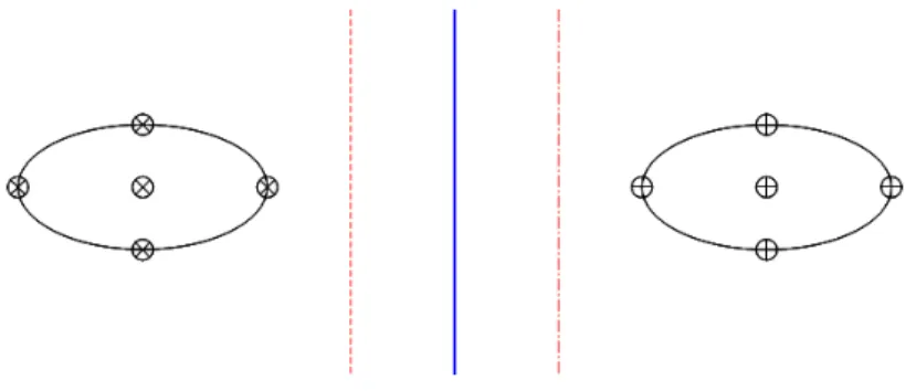
Example 2.4. Consider the totally separable binary classification problem described in Figure 1. Here,⊕ repre-sents the samples in one category, and⊗represents the samples in the other category. We choose the solid line in
Fig. 1. Demo: Multiple solutions for LP (2)
can be decided and we denote the values asw and¯ b, respectively. For all i¯ = 1,· · ·, , if yi(xTiw¯ +b¯) ≥0, let ¯
ξi =0andβ¯i=yi(xTiw¯+b¯); if yi(xTiw¯ +b¯)<0, letβ¯i =0andξ¯i=−yi(xTiw¯ +b¯). It can be easily checked that ( ¯wT,b¯,ξ¯T,β¯T)T ∈ n+2+1satisfies all the constraints in (2). Therefore, a feasible point(wT,b,ξ¯T,β¯T)T ∈Ω
1 of
LP (2). Since this is a totally separable problem, for all i=1,· · ·, , we haveξ¯i=0andβ¯i >0, a feasible point
with the negative function value is then constructed.
Summarizing the discussion above, we can see that for the totally separable problem, for any value ofγ >0, LP (2) is unbounded, i.e. LP (2) is always unsolvable. Unfortunately, this is not the only unwanted situation we might meet. The following example demonstrates another fetal defect of solving MCLP (1) by LP (2).
Example 2.5. Consider again the classification problem depicted in Figure 1. The solid line in the middle of the figure, the dash line in the left hand and the dash-dot line in the right hand are all separating planes. And obvious-ly, the solid line in the middle is the best separating plane one can find. Following the constructive way in Example 2.4, denote the feasible point corresponds to the solid line as(wT,b¯,ξ¯T,β¯T)T, the feasible point corresponds to the
dash line as(wT,b´,ξ´T,β´T)T, and the feasible point corresponds to the dash-dot line as(wT,b`,ξ`T,β`T)T.1 Though
simple computations, we can see that the objective function value of LP (2) for these three different points are the same. This means that if(wT,b¯,ξ¯T,β¯T)T is the optimal solution of LP (2), so are the points(wT,b´,ξ´T,β´T)T and (wT,b`,ξ`T,β`T)T. Then according to LP (2), all three separating planes are the best separating plane, which is, obviously, not the result we want to get.
In all, we can see that LP (2) is not a good model for the totally separable classification problem. Since the totally separable case is the ideal and the simplest situation in classification, in order to apply LP (2) successfully, we have to make some modification.
2.3. New Regularized MCLP Model for Binary Classification
Just as we have discussed in the above subsection, LP (2) might be unsolvable. In the exiting works for solving MCLP by LP (2)[12, 13, 14, 15, 17], this trap is avoided by pre-setting the value of part of the variables in LP (2). However, if the chosen value are not proper, even LP (2) can be solved, the separating plane obtained may still not be a good separating plane. From this point of view, the choice for the value of the pre-setting variables is very important. Heuristic search and expert knowledge are always necessary for deciding a good value, which is timing consuming and limits the applications of MCMP to some extend. So in this paper, we would like provide a new method to guarantee the solvability instead of the way of fixing the value of part of the variables.
In order to avoid the difficulty described in Example 2.5, we suggest adding a regularization term12βTHβinto the objective function of (2), whereHis a×positive matrix. Then we obtain the following modified formulation for the LP (2), which is a quadratic programming:
min w,b,ξ,β i=1ξi−γ i=1βi+ 1 2τβTHβ (3a) s.t. yi(xTiw+b)=βi−ξi,i=1,· · · , ; (3b) ξi≥0, βi≥0, i=1· · · , ; (3c)
whereτ >0 is a pre-given parameter. The following theorem shows that the solvability of the modified problem (3) is guaranteed.
Theorem 2.6. Problem (3) always has a feasible solution.
Proof. BecauseHis positive definite, for allβ∈ , the minimum value of−γli=1βi+12βTHβis−γ
2
2τe TH−1e. Becauseξ ≥ 0, we have thatli=1ξi ≥ 0. In all, we know for problem (3), the objective function has a lower bound−γ22τeTH−1e. We notice that the feasible set of LP (2) is the same as quadratic program (3, from Lemma 2.1 we know that the feasible set of problem (3) is nonempty. In all, we obtained the conclusion that the optimization problem (3) always has a feasible solution.
Consider again the example in Figure 1. LetH=I, it can be easily checked that for (model 3), only the solid line in the middle corresponds to the optimal solution and the situation described in Example 2.5 does not happen. Compared with the regularized MCLP proposed in [16], in (3), there is only one quadratic regularization term in the objective function. So fewer regularization parameter and matrix need to be tuned in our modified formulation and, therefore, our method is cheaper to be implemented in practice.
Although problem (3) always has finite optimal solutions, there is still an defect from the modeling point of view. In details, we notice that
xTw+b=0 andtxT+tb=0, for allt>0
presents the same discriminant function and therefore, the same separating plane. However, the objective function value of (3) corresponds totxT+tb=0 differs with the value oft>0, which is obviously should not occur. As a remedy to this problem, we should require that the slope-intercept expression of each discriminant function is unique in the model. This requirement can be easily implemented by choosing the value of intercept termbfrom the set{1,0,−1}. Then we get the following model of mixed integer nonlinear programming:
min w,b,ξ,β l i=1ξi−γli=1βi+12τβTHβ (4a) s.t. yi(xTiw+b)=βi−ξi,i=1,· · ·, ; (4b) ξi≥0, βi≥0, i=1· · ·, ; (4c) b∈ {−1,1,0}. (4d)
We observe that ifxTw∗ =0 is the best separating plane, where the value of||is small enough,xTw∗+ =0 is also a good enough separating plane. Since as long as the intercept term is not zero, it is always can be normalized to 1 or -1. To reduce the computational cost further, we can omitted the case ofb=0 from (4) and suggest users apply the following simplified model in practice:
min w,b,ξ,β l i=1ξi−γli=1βi+12τβTHβ (5a) s.t. yi(xTiw+b)=βi−ξi,i=1,· · ·, ; (5b) ξi≥0, βi≥0, i=1· · ·, ; (5c) b∈ {−1,1}. (5d)
Sometimes, considering the stability of calculations, the users may favor the separating plane whose elements in slope is not too large. To this aim. the regularization termκwTKwcan be added to the objective function to limit the value of the elements inw. Then the following model can be considered instead of (5):
min w,b,ξ,β l i=1ξi−γ l i=1βi+12τβTHβ+12κwTKw (6a) s.t. yi(xTiw+b)=βi−ξi,i=1,· · ·, ; (6b) ξi≥0, βi≥0, i=1· · ·, ; (6c) b∈ {−1,1}, (6d)
whereκ >0 and positive matrixK∈ n×nare pre-given model parameters. Similar to the proof in Theorem 2.6, we can easily proved that the solvability of both model (5) and (6) can be guaranteed.
3. Experiments
To test the performance of the new method, we compared our algorithm with several state-of-the-art algorithms for binary classification in this section. All experiment were executed on a computer with Intel I5 CPU, CPU clock rate of 3.10GHz, 2 GB main memory. The method proposed in this paper are solved byCVX[19, 20], which is a Matlab-based modeling system for convex optimization. CVX are described using a limited set of construction rules, which enables them to be analyzed and solved efficiently. As for the implementation for other algorithms,
SVM were applied withlibSVM[21] which is an powerful software for both support vector classification and regression; Other typical methods were implemented throughWeka [22] platform, which is an excellent data mining environment that integrates various of machine learning algorithms under a uniform platform.
The datasets in our experiment are all from the UCI Machine Learning Repository [23]. Most of them are wildly used for machine learning research in the validation and comparison among classification algorithms. For each dataset, we first discarded the instances with missing value. And then, grid search were adopted to selecting proper parameters for each method. Search procedure were executed under an uniform settings. During searching we chose 5 fold cross-validation for each group of parameters. That is to say, for each parameters group candidate, classification accuracy was obtained once by running a 5-fold cross validation on a specific dataset. After all, we chose the best accuracy as the performance of the method on that dataset. Several classical binary classification algorithms were chosen for comparison including linear SVC [8], Naive Bayes [24], C45 [25], Random Forest [26] and KNN [27]. The experimental results were showed in Table 1. Here, the column “RMCLP1” and “RMCLP2” represents the results for the model (5) and (6), respectively.
Table 1. Classification Accuracy Result Comparison in different datasets
ID Ins Num Attri Num RMCLP1 RMCLP2 LinearSVC NaiveBayes C45 RandomForest KNN
iris 0 1 100 4 100 100 100 100 99 100 100 iris 0 2 100 4 100 100 100 100 100 100 100 iris 1 2 100 4 99 97 97 91 92 93 96 wine 0 1 130 13 99.3 97.69 100 98.46 93.08 100 98.46 wine 0 2 107 13 100 100 100 100 99.07 100 100 wine 1 2 119 13 100 100 99.16 97.48 94.12 99.16 96.64 breast-cancer 277 9 75.09 75.45 73.29 73.29 75.45 72.2 75.09 breast-w 683 9 97.22 97.36 97.36 96.19 95.46 97.36 97.36 credit-a 653 15 88 87.6 86.52 78.1 85.15 86.22 87.29 credit-g 1000 20 76.1 76.6 76.5 74.8 71.4 75.3 73.8 diabetes 768 8 77.6 77.47 78.52 75.39 72.4 77.21 74.22 heart-statlog 270 13 86.3 86.67 85.19 82.96 80.37 81.48 81.48 hepatitis 80 19 90 90 91.25 85 77.5 88.75 86.25 ionosphere 351 34 88.03 89.17 89.46 82.62 89.74 94.3 88.89 liver-disorders 345 6 70.73 71.01 71.88 57.1 66.67 73.04 63.19 sonar 208 60 82.21 79.81 81.25 66.83 68.75 85.1 86.06 spambase 4601 57 91.98 92.52 93.11 79.55 93.13 95.87 90.68 Average 89.5 89.31 89.44 84.63 85.48 89.35 87.96
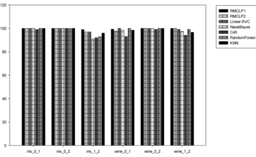
In order to validate how our algorithm works in separable cases, we turned two simple datasets ‘iris’ and ‘wine’ into binary classification problems by having two of their original categories left. In general, good classifiers should almost make this kind of datasets completely divided. Experiment results are illustrated in Figure 2. In details, the leftmost two bars in Figure 2 representing the performance of our method, from which we can see that separable data indeed can be identified and well treated by our regularization method. By comparing with other five bars in the figure, we can find that our method perform as well as other classical algorithms.
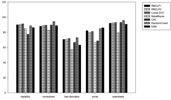
Then we compare our regularized model with the state-of-the-art algorithms in the non-separable cases. The results in figure 3 and 4 show that our method is still competitive with other algorithms confronting more complex situation. Especially, for the datasets ‘credit-a’, ‘credit-g’ and ‘heart-statlog’, our method obtains the highest classification accuracy among all the algorithms. One of the possible reason for this result is that in these three datasets, there is linear relationship among some features of the samples, and our method can explore this kind of linear correlation better than other methods. Furthermore, The results on the different types of data also illustrate the stability of our method.
4. Conclusion and future work
MCLP, as an alternative method for classification and regression, has been widely used in various machine learning and data mining problems. In order to apply MCLP efficiently in practice, many methods convert the
Fig. 2. Comparison on separable datasets
Fig. 4. Comparison on more complex datasets 2
original MCLP into a objective linear program to solve. However, the solvability of the converted single-objective optimization is not very clear. In this paper, we take the MCLP for binary classification as the example and discuss how to modified the formulation of converted single-objective optimization to guarantee the solvabil-ity. By fixing the value of intercept of the separating plane to{±1}, the new model overcomes some defects of the original scalarized problem in modeling; By adding a quadratic regularization term into the objective function, the new regularized formulation can be shown that the finite optimal solutions always exist. We compare the new method with several state-of-the-art algorithms for binary classification on several different kinds of datasets. Preliminary experimental results indeed demonstrate the effectiveness of our method.
The model proposed in this paper is restricted to the case with linear kernel. Although we know linear classifier is a good choice for lots of practical applications, especially for those whose dimension of the input feature is very high. There are still quite a few problems cannot be predicted accurately by linear functions. Therefore, in order to exploit the flexibility of nonlinear separating surfaces, we plan to extend the model to the case with nonlinear kernels, which is interesting and very changeable. To the best of our knowledge, there is no existing work for regularized MCLP with nonlinear classifiers currently. In this paper, we only considered the case of binary classification in this paper. How to apply the idea to more general cases, such as multi-category classification or regression, is also one of our on ongoing works.
Acknowledgement
This work was partially supported by the National Natural Science Foundation of China(Grant No. 11201472, 11026187, 70921061, 10831006),the president fund of the Graduate University of Chinese Academy of Sciences( Grant No. Y15101PYOO), and the CAS/SAFEA International Partnership Program for Creative Research Team-s(Grant No. kjcx-yw-s7).
References
[1] A. Charnes, W. W. Cooper, Management models and industrial applications of linear programming, Management Science 4 (1) (1957) 38–91.
[2] J. B. Rosen, Pattern separation by convex programming, Technical report AD0416795, Standford University (June 1963).
[4] N. Freed, F. Glover, Simple but powerful goal programming models for discriminant problems, European Journal of Operational Re-search 7 (1) (1981) 44–60.
[5] N. Freed, F. Glover, Evaluating alternative linear programmning models to solve the two-group discriminant problem, Decision Science 17 (2) (1986) 151–162.
[6] B. Boser, I. Guyon, V. Vapnik, A training algorithm for optimal margin classifiers, in: COLT92: Proceedings of the Fifth Annual Workshop on Computational Learning Theory, ACM press, New York, NY, 1992, pp. 144–152.
[7] C. Cortes, V. Vapnik, Support vector networks, Machine Learning 20 (3) (1995) 273–297. [8] V. Vapnik, The Nature of Statistical Learning Theory, Springer, New York, NY, 1995. [9] V. Vapnik, Statistical Learning Theory, Wiley-Interscience, New York, 1998.
[10] Z. Qi, Y. Xu, L. Wang, Y. Song, Online multiple instance boosting for object detection, Neurocomputing 74 (10) (2011) 1769–1775. [11] Z. Qi, Y. Tian, S. Yong, Robust twin support vector machine for pattern classification, Pattern Recognition 46(1) (2013) 305–316. [12] Y. Shi, Multiple criteria optimization based data mining methods and applications: A systematic survey, Knowledge and Information
Systems 24 (3) (2010) 369–391.
[13] G. Kou, X. Liu, Y. Peng, Y. Shi, M. Wise, W. Xu, Multiple criteria linear programming to data mining: Models, algorithm designs and software developments, Optimization Methods and Software 18 (2003) 453–473.
[14] Y. Shi, Y. Peng, G. Kou, Z. Chen, Classifying credit card accounts for business intelligence and decision making: A multiple-criteria quadratic programming approach, International Journal of Information Technology and Decision Making 4 (2005) 581–600.
[15] Y. Peng, G. Kou, Y. Shi, Z. Chen, A multi-criteria convex quadratic programming model for credit data analysis, Decision Support Systems 44 (2008) 1016–1030.
[16] Y. Shi, J. Tian, X. Chen, P. Zhang, Regularized multiple criteria linear programs for classification, Science in China Series F: Information Sciences 52 (2009) 1812–1820.
[17] J. He, Y. Zhang, Y. Shi, G. Huang, Domian-driven classification based on multiple criteria and multiple constraint-level programming for intelligent credit scroing, IEEE Transactions on Knowleage and Data Engineering 22 (6) (2010) 826–838.
[18] P. L. Yu, A class of solutions for group decision problems, Management Science 19 (8) (1973) 936–946. [19] M. Grant, S. Boyd, CVX: Matlab software for disciplined convex programming, version 1.21 (2011).
[20] M. Grant, S. Boyd, Graph implementations for nonsmooth convex programs, in: V. Blondel, S. Boyd, H. Kimura (Eds.), Recent Advances in Learning and Control, Lecture Notes in Control and Information Sciences, Springer-Verlag Limited, 2008, pp. 95–110.
[21] C.-C. Chang, C.-J. Lin, LIBSVM: A library for support vector machines, ACM Transactions on Intelligent Systems and Technology 2 (2011) 27:1–27:27, software available athttp://www.csie.ntu.edu.tw/~cjlin/libsvm.
[22] M. Hall, E. Frank, G. Holmes, B. Pfahringer, P. Reutemann, I. H. Witten, The weka data mining software: an update, SIGKDD Explor. Newsl. 11 (1) (2009) 10–18.
[23] A. Frank, A. Asuncion, UCI machine learning repository,http://archive.ics.uci.edu/ml, university of California, Irvine, School of Information and Computer Sciences (2010).
[24] G. H. John, P. Langley, Estimating continuous distributions in bayesian classifiers, in: Eleventh Conference on Uncertainty in Artificial Intelligence, 1995, pp. 338–345.
[25] G. Webb, Decision tree grafting from the all-tests-but-one partition, Morgan Kaufmann, San Francisco, CA, 1999. [26] L. Breiman, Random forests, Machine Learning 45 (1) (2001) 5–32.