EE 508 Lecture 11. The Approximation Problem. Classical Approximations the Chebyschev and Elliptic Approximations

EE 508

Lecture 11

The Approximation Problem

Classical Approximations

Butterworth Approximations

• Analytical formulation:

–

All pole approximation

–

Magnitude response is maximally flat at ω=0

–

Goes to 0 at ω=∞

–

Assumes value at ω=1

–

Assumes value of 1 at ω=0

–

Characterized by {n,ε}

• Emphasis almost entirely on performance at

single frequency

"On the Theory of Filter Amplifiers", Wireless Engineer (also called

Experimental Wireless and the Radio Engineer), Vol. 7, 1930, pp. 536-541.

2 1 1 Review from Last Time

1 1 ω   LP T j

Butterworth Approximation

Poles of T_BW(s)









1/ 1 sin 1 2 cos 1 2 2 2 n k p k j k n n      _ _  _ _  _   1 n k=0,1, ... 2  for n even     1/ _{sin 1 2 cos 1 2} 2 2 n k p k j k n n          _ _  _ _  _      





1/ 1 0 n n p    j n-3 k=0, ... 2 for n odd Re Im n  1 n     Re Im n  1 n     Review from Last Time

Butterworth Approximation

What is the Q of the highest Q pole for the BW approximation?

1/ 0 sin cos 2 2 n p j j n n            _ _{ } _{ }        Re Im n  1 n     Highest Q Pole 2 2 2 MAX Q       1 1 2 2 sin cos 1 2 2 2 sin 2sin 2 2 n n MAX n n Q n n        _                         1 2sin 2 MAX Q n        

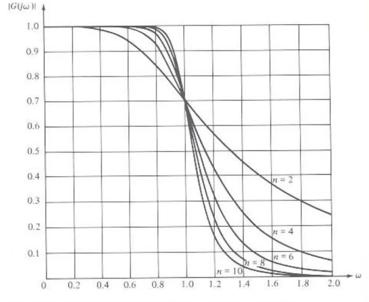
Butterworth Approximation

Order needs to be rather high to get steep transition

Figure from Passive and Active Network Analysis and

Synthesis, Budak Re v iew from Las t T ime

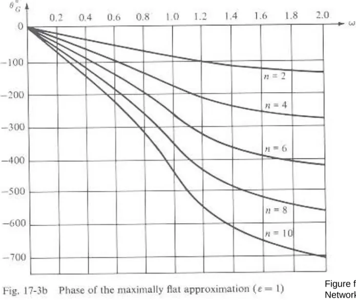
Butterworth Approximation

1 2 2sin 2n        

Phase is quite linear in passband (benefit unrelated to design requirements)

Figure from Passive and Active Network Analysis and

Synthesis, Budak Re v iew from Las t T ime

Butterworth Approximation

• Widely Used Analytical Approximation • Characterized by {ε,n}

• Maximally flat at ω=0

• Almost all emphasis placed on characteristics at single frequency (ω=0) • Transition not very steep (requires large order for steep transition)

• Pole Q is quite low

• Pass-band phase is quite linear (no emphasis was placed on phase!) • Poles lie on a circle

• Simple closed-form analytical expressions for poles and |T(jω)|

Summary Re v iew from Las t T ime

Approximations

• Magnitude Squared Approximating Functions – H

_A

(ω

2

)

• Inverse Transform - H

_A

(ω

2

)→T

A

(s)

• Collocation

• Least Squares Approximations

• Pade Approximations

• Other Analytical Optimizations

• Numerical Optimization

• Canonical Approximations

– Butterworth

– Chebyschev

– Elliptic

– Bessel

– Thompson

1 1 ω   LP T j

Pafnuty Lvovich Chebyshev

Born May 16, 1821

Died December 8,1894

Nationality Russian

Chebyshev Approximations

• Analytical formulation:

–

All pole approximation

–

Magnitude response bounded between 1 and

in the pass band

–

Assumes the value of at ω=1

–

Goes to 0 at ω=∞

–

Assumes extreme values maximum no times in [0 1]

–

Characterized by {n,ε}

• Based upon Chebyshev Polynomials

Chebyshev polynomials were first presented in: P. L. Chebyshev (1854) "Théorie des mécanismes connus sous le nom parallelogrammes," Mémoires des Savants

étrangers présentes à l'Academie de Saint-Pétersbourg, vol. 7, pages 539-586.

2 1 1 2 1 1

Type I Chebyshev Approximations

1 1 ω   LP T j

Chebyshev Approximations

• Analytical formulation:

–

Magnitude response bounded between 0 and

in the stop band

–

Assumes the value of at ω=1

–

Value of 1 at ω=0

–

Assumes extreme values maximum times

in [1 ∞]

–

Characterized by {n,ε}

• Based upon Chebyshev Polynomials

2 1    2 1 1

Type II Chebyshev Approximations (not so common)

1 1 ω   LP T j

Chebyshev Approximations

Chebyshev Polynomials

The Chebyshev polynomials are characterized by the property that

the polynomial assumes the extremum values of 0 and 1 a maximum number of times in the interval [0,1] and go to ∞ for x large.

In polynomial form they can be expressed as C₀(x)=1

C₁(x)=x

C_n+1(x)=2xC_n(x) - C_n-1(x)

Or, equivalently, in trigonometric form as

 

 





 





 



 



cos cos [ 1,1] cosh cos 1 1 cosh cos 1 n n n arc x x C x n arc h x x n arc h x x  _{  }   _        

Chebyshev Approximations

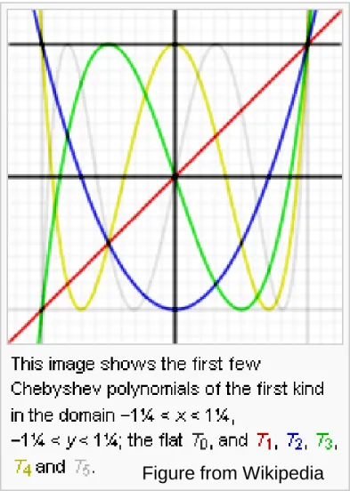
Chebyshev Polynomials

Figure from Wikipedia

 

 

 

 

 

 

 

 

 

0 1 2 2 3 3 4 2 4 5 3 5 6 4 2 6 7 5 3 7 8 6 4 2 8 1 2 1 4 3 8 8 1 16 20 5 32 48 18 1 64 112 56 7 128 256 160 32 1 C x C x x C x x C x x x C x x x C x x x x C x x x x C x x x x x C x x x x x                         

The first 9 CC polynomials:

• Even-indexed polynomials are functions of x2

• Odd-indexed polynomials are product of x and function of x2

Chebyshev Approximations

Type 1

 

BW _{2 2n}

1

H

ω =

1+



ω

 

 

2 2 n

1

H

ω =

1+



F

ω

Butterworth _{A General Form}

F_n(ω2_{) close to 1 in the pass band and gets very large in stop-band}

Observation:

The square of the Chebyshev polynomials have this property

 

 

CC

2 2

n

1

H

ω =

1+



C

ω

Chebyshev Approximations

Type 1

 

 

CC

2 2

n

1

H

ω =

1+



C

ω

Im Re Poles of H_CC(ω) lie on an ellipse with none on the real axis

Chebyshev Approximations

Type 1

 

 

CC

2 2

n

1

H

ω =

1+



C

ω

Im Re Im Re Poles of T_CC(s) Inverse Mapping

Chebyshev Approximations

Type 1 Im Re 2 2 1 1 1

sinh 1 sinh cosh 1 sinh

n n k k arc arc                                      _{  }  _{  }    

Chebyshev Approximations

Type 1 Im

Re

Poles of T_CC(s)





1 1





1

sin sinh cos cosh

k π π 1 p 1+2k sinh 1+2k sinh 2n narc  j 2n narc                _{    } _{    }           k p  _k  j_k 2 2 1 1 1

sinh 1 sinh cosh 1 sinh

n n k k arc arc                                      _{  }  _{  }    

Properties of the ellipse

Chebyshev Approximations

Type 1 ω 1 2 1 1

 

CC T ω Even order 1 2 1 1 ω 1

 

CC T ω Odd order

• |T_CC(0)| alternates between 1 and with index number • Substantial pass band ripple

• Sharp transitions from pass band to stop band

2 1 1

Chebyshev Approximations

Type 1

Sharp transitions from pass band to stop band

Chebyshev Approximations

Type 1

CC transition is much steeper than BW transition From Budak Text

Comparison of BW and CC

Responses

• CC slope at band edge much steeper than that

of BW

• Corresponding pole Q of CC much higher than

that of BW

• Lower-order CC filter can often meet same

band-edge transition as a given BW filter

• Both are widely used

• Cost of implementation of BW and CC for same

order is about the same

1

1

2 2

(

)

[

(

)]

CC BW

n

Slope



 











n



Slope









Chebyshev Approximations

Type 1

From Budak Text

Analytically, it can be shown that, at the band-edge

 





2 3 2 2 1 BW d T j n d  _    _  





2 3 2 2 2 1 CC d T j n d  _    _

Chebyshev Approximations

Type 1

CC phase is much more nonlinear than BW phase From Budak Text

Chebyshev Approximations

Type 1 Im

Re





1 1





1

sin sinh cos cosh

k π π 1 p 1+2k sinh 1+2k sinh 2n narc  j 2n narc                _{    } _{    }          

Maximum pole Q of CC approximation can be obtained by considering pole with index k=0

1 1 1

sin sinh cos cosh

0 π π 1 p sinh sinh 2n narc  j 2n narc                _{    } _{    }           2 2 2 MAX Q       0 p =  j Recall 2 cos 1 1 1 2sin sinh MAX,CC π 2n Q π 1 sinh 2n narc              _{ }             _{ }  _{ } _   _      

Chebyshev Approximations

Type 1

Comparison of maximum pole Q of CC approximation with that of BW approximation

2 cos 1 1 1 2sin sinh MAX,CC π 2n Q π 1 sinh 2n narc              _{ }             _{ }  _{ } _   _       1 2sin 2 MAX,BW Q n         2 cos 1 1 sinh MAX,CC MAX,BW π 2n Q Q 1 sinh narc   _{ }     _{ }                _{  }  

Example – compare the Q’s for n=10 and ε=1 Q_BW=3.19 Q_CC=35.9

Chebyshev Approximations

Type 2

 

BW _{2 2n}

1

H

ω =

1+



ω

 

 

2 2 n

1

H

ω =

1+



F

ω

Butterworth _{A General Form}

 

 

1

CC2

2 2

n

1

H

ω =

1

1+

C

ω



Another General Form

 

 

2 2 n

1

H

ω =

1

1+

F 1/ω



Note: The second general form is not limited to use of the Chebyshev polynomials

Chebyshev Approximations

Type 2

 

 

1

CC2 2 2 n

1

H

ω =

1

1+

C

ω



• Equal-ripple in stop band • Monotone in pass band

• Both poles and zeros present

• Poles of Type II CC are reciprocal of poles of Type I

• Zeros of Type II are inverse of the zeros of the CC Polynomials





1

cos

π

2k-1

2

n

k

z



j





















1 1 1 1

sin sinh cos cosh

k p π π 1 1+2k sinh 1+2k sinh 2n narc  j 2n narc            _                          

Chebyshev Approximations

Type 2

 

 

1

CC2 2 2 n

1

H

ω =

1

1+

C

ω



1 2 1 1 1  

 

CC T ω Odd order 2 1 1 1   1

 

CC T ω Even order

Chebyshev Approximations

Type 2

 

 

1

CC2 2 2 n

1

H

ω =

1

1+

C

ω



1 2 1 1 1  

 

CC T ω

• Transition region not as steep as for Type 1 • Considerably less popular

Chebyshev Approximations

Type 2

 

 

1

CC2 2 2 n

1

H

ω =

1

1+

C

ω



• Pole Q expressions identical since poles are reciprocals • Maximum pole Q is just as high as for Type 1

1 Re Im 1 Re Im